A Fast and Stable Cluster Labeling Method for Support Vector Clustering

A Fast and Stable Cluster Labeling Method for

Support Vector Clustering

Huina Li

Department of Computer Science and Technology, Xuchang University, Xuchang 461000, China Email: [email protected]

Abstract— Even though support vector clustering (SVC) is able to handle arbitrary cluster shapes effectively, its popularity is frequently degraded by highly intensive time complexity, poor label performance and even instability for efficiency. To overcome such problems, a fast and stable cluster labeling (FSCL) method is proposed. Based on stable equilibrium points, the FSCL first finds an appropriate di-vision of support vectors. With a nonlinear sample sequence strategy presented here, the connected components profiled by support vectors (SVs) can be determined in terms of sampling all stable equilibrium point pairs; and the FSCL prefers a density centroid constructed by one subset of SVs, along with a stable equilibrium point, to represent a component while avoiding local optimization. Finally, the remaining data points can be assigned the label of the nearest components with respect to a weighted distance. Time complexity analysis and comparative experiments suggest that the FSCL improves both the efficiency and clustering quality significantly while guaranteeing stability.

Index Terms— support vector clustering, centroid, stable equilibrium point, unsupervised learning method, support vector machine

I. INTRODUCTION

Clustering, focusing on forming natural grouping of data points that maximize intro-cluster similarity and minimize inter-cluster similarity, has been extensively employed in image processing, pattern recognition, data analysis and instance-based learning, etc. Among the pre-vious studies [1], [2], support vector clustering (SVC) [3]– [7], a boundary-based clustering algorithm inspired by the support vector machines (SVM) [8] whose advantage is to generate cluster boundaries of arbitrary shape, is recently emerged algorithm to characterize the support of a high-dimensional distribution.

Given a dataset X with N points {x1,x2, . . . ,xN}, two main phases are included by SVC to cluster these data points, i.e., SVC training to estimate a support function by solving a dual problem and cluster labeling to assign each data point to its corresponding cluster. Apparently, both of the two phases can be considered as bottlenecks to the SVC’s application since too much time is frequently required. However, along with some

Manuscript received Mar 14, 2013; revised April 2, 2013; accepted April 16, 2013. c⃝2005 IEEE.

This work is supported by the Foundation of He’nan Education-al Committee under Grant No. 13A413750, 13A413747, the NaturEducation-al Science Foundation of He’nan Province of China under Grant No. 132300410393, 122102210543, and Xuchang Municipal Natural Science Foundation under Grant No. 5018, 1101030, 1101059.

insightful techniques employed by the first phase, e.g., chunking [9], problem transferring [10], [11], noise and core points elimination [12], [13], the cluster labeling phase with time complexity of O(N2_{m) takes most of}

the computation time for the entire SVC process. Here, mis the sample rate for each point pair. Thus, it is crucial to make improvement on efficiency of the labeling step, especially for large-scale problems purpose. To achieve this objective, based on the complete graph (CG) strategy [3], a number of insightful works have been done, i.e., the support vector graph (SVG) [4], proximity graph of delaunay (DD) [14], minimum spanning tree (MST), k-nearest neighbor (kNN) [15], [16], divide and conquer-based methods [17], [18], cell growth conquer-based method [19], cone cluster labeling (CCL) [20], [21], and equilibrium based approaches [22]–[28].

Despite so many variants have been developed, there are still difficulties to achieve efficiency, accuracy and stability. For instance, even though reduced complete graph (R-CG) [22] reached significantly improvement on efficiency, it suffers from too many local minimums, ineffectively dealing with irregular clusters. Then equilib-rium based support vector clustering (E-SVC) [23]–[25] was proposed to make further improvement on accuracy, but the pricey time consumption degrades its application. Furthermore, fast support vector clustering (FSVC) [28], a recent insightful variant of SVC, constructs an amount of small balls using the whole dataset, looks for stable equilibrium vectors (SEVs) for connective analysis from the centers of balls separately. Despite of time consump-tion reduced significantly, FSVC suffer from instabilities mainly due to the assumption of circular distribution of clusters. As another achieved method, a very fast calculation of adjacency matrix of SVs can be made by CCL. Unfortunately, a strict constraint condition to guarantee the radius of hypersphere to be lower than 1 seriously increases its time complexity of solving dual problem.

main contributions lie in three aspects:

1) To reduce the account of sampled point pairs, only the SVs are selected to locate the SEVs before finding connected components since they do profile clusters ac-curately.

2) For efficiency, the work of finding the connected components is done between the SEV pairs. More im-portantly, the average sample rate is significantly reduced according to a novel proposed strategy of disconnection checking first.

3) To assign the remaining data points correctly, a pair of data points, i.e., a SEV and a density centroid, are constructed to achieve a better support of any shape and distribution of a component. Then the remaining data points could be labeled following the principle of max-imum subordinated degree among the components with a weighted distance in the input space. Time complexity analysis and comparative experiments with the state-of-the-art methods suggest that the FSCL improves both the efficiency and clustering quality significantly. Moreover, it is stable.

The remainder of this paper is arranged as follows. We formally introduces the framework of the FSCL in Section II. Compared with the traditional ones, Section III details the evaluations with respect to accuracy and efficiency. Finally, the last section draws conclusions for this study with the future work.

II. THEFAST ANDSTABLECLUSTERLABELING ALGORITHM

To well describe the proposed FSCL algorithm, three essential phases with novel strategies, i.e., decomposition of SVs by SEVs, connectivity analysis of components and cluster assignments for non-SVs, are adopt to be detailed in this section.

A. Phase I. Partition of SVs

Suppose that the set of SVs are denoted byV(V ⊆ X), from the principle of SVC, the image of any SV, e.g.,

Φ(v)(v ∈ V), lies on the surface of the feature space sphere and has an unique distanceRto the hypersphere’s center α. Here Φ(·) is a nonlinear transformation. That is to say the distance from any data point lies in the profile to α is always lower than R. Following closely the derivation of [22]–[24], [26], to obtain the solution of the minimal hypersphere approximate covering with an appropriate width qof the kernel function, a gradient dynamical system which is associated with the trained kernel function R2_{(x)can be constructed as follows.}

R2(x) =||Φ(x)−α||2 (1)

∂x

∂t =−∇R

2_(x)

(2)

In Eq.(1), there exists a unique solution (or trajectory)

x(·) : R → Rn for each condition x(0) = x0 is guaranteed since it is twice differentiable and the norm of

∇R2_{(x)is bounded. Moreover, a SEVx¯ can be obtained}

if the equation∇R2_{(¯x) = 0and all the eigenvalues of its}

corresponding Jacobian matrix, JR(¯x) ≡ ∇2_R2_{(¯x), are}

positive. Since the cluster boundaries consist of SVs, in order to achieve improvement on efficiency, only SVs are selected to get a unique partition of SVs that satisfies the Theorem 1.

Theorem 1: In terms of the gradient dynamic system (2), the dataset of SVs V can be partitioned into sev-eral separate and non-overlapped subsets with respect to SEVs, i.e.,

V =

Nc

∪

i=1

Vi

s.t. lim

vik∈Vi,k∈[1,Ni]

t_→∞

vi(t) =xi, Vi∩Vj=∅,

for ∀i, j∈[1, Nc], i̸=j

(3)

wherexiis the SEV corresponding toVi,Nc andNi are the number of subsets and SVs in Vi respectively.

Proof: Proved by Ref. [22], [28], [29], all the data points can be grouped by different convergence objects which are the local minimum positions reached from the points with respect to the dynamic system. Furthermore, the local minimum position is unique for each point, so the decomposed data sets are non-overlapping.

B. Phase II. Connectivity Analysis of Components

In geometry, the region whose boundary is built up by Vi is considered as a component (denoted by Ci) for further connectivity analysis. Since these SEVs locate inside components with a local minimum distance to the center α of hypersphere while being mapped into feature space, naturally, the nearer a data point is away from a SEV, the less impossible it locates outside a component. Thus, for efficiency, a disconnection checking first strategy is presented in this section.

S1

S2 S3

S4

A

B

o

¡¡! S₁A

á¡

S

4B

OĄ

(a) Sampling SEVs pairs for adjacency martix

S

S

2

1 3 4 5 6 7 8 9

(b) Nonlinear sample sequence

Figure 1: Principle of disconnection checking first strate-gy.

SEVs (i.e., S1,S2,S3,S4) have been found, the connection

status of their corresponding components can be checked by sampling line segments connecting each SEV pairs, e.g., S1S4, S1S2, etc. Generally, the conventional methods

[3], [4], [13], [19], [22]–[25], [27], [28] prefer a linear sample sequence from one side to the other, for instance, either −−→S1S4 or −−→S4S1. Apparently, redundant segmers can

not be avoided, e.g., segmers on line segments S1Aand

S4B. Therefore, a nonlinear sample sequence generated by

a disconnection checking first strategy, shown in Fig.1(b), is proposed in a simple but rather more effective way. Consider the line segment connecting two SEVs (i.e., S1S2), it is split into m segmers, for instance, m = 1

while m−1 points are expected to be checked. Among these sample points, the center of the line segment (i.e., 5) is selected as initial point and to be check first; then the distance from each sample point to the initial point is increase gradually. In the worst case, the full sample sequence is{5, 6, 4, 7, 3, 8, 2, 9, 1}. If two components are strongly disconnected or not connected directly like that of corresponding to S1,S2, only one sample point

might be sufficient for giving the final decision correctly.

C. Phase III. Cluster assignments for non-SVs

Generally, the remaining data points would be labeled by their nearest neighboring SVs or SEVs. However, since the locations of SVs are determined by the parameters [4], i.e., kernel width q and penalty factor C, and the SEVs usually are at the center of their corresponding components’ profiles, they are not sufficient for judging a data point with relatively balanced membership grades to multiple neighboring components. So, in addition to SEV, inspired by Ref. [30], a kind of density centroid is defined for representing a component.

Definition 1 (density centroid): The density centroid (denoted by DC) is a logic data point defined by formula (4) for a component:

DC(Ci) =

1

Ni Ni

∑

i=1

vi, ∀vi∈Vi (4)

where Ni is the number of SVs in subset Vi w.r.t. component with SEVSi.

Actually, the density centroid get close to the highest density position of a component but usually not overlap with the SEV. The greater the gap of the distance be-tween them, the much more imbalanced distribution for the component is. Consider unequal contributions from them, a simple linear programming problem (Eq.(5)) is constructed and solved by a series of SVs to quantify the weight of each points.

min 1

Ni Ni

∑

i=1

(WSi ∥xi−Si∥ 2₊

WDC(SCi)∥xi−DC(Ci)∥2) 1 2

s.t. WSi+WDC(Ci)= 1

WS_i ≥1

2, WDC(Ci)≥0

(5)

In Eq.(5),WS_i andWDC(Ci)are the weight of

contribu-tions from SEV Si and density centroidDC(Si)in Ci, respectively. Notice thatWS_i ≥1₂ is set to emphasize the contribution of SEVs. Based on the extracted weights, a number of weighted norm distances from each remaining data point x to component Ci(i ∈ [1, Nc]) could be achieved; and then x would be assigned with the label of its nearest component with the minimum weighted norm distance detailed by Eq.(6). In order to get the two euclidean distances between x and any component, the computation taken in the input space is recommended for efficiency.

label(x) =label(arg min

Si

(WS_i ∥x−Si∥2+

WDC(Ci)∥x−DC(Ci)∥2)

1 2₎

(6)

D. Implementation and Time Complexity

Algorithm 1 shows the FSCL method. In line 1, for the given q and C, it collects the SVs by solving the dual problem. Then V is split while their corre-sponding SEVs (denoted by SSEVs) are obtained

ac-cording to LocateSEVsbySVs(SSEVs) detailed in section

II-A. In line 3, the adjacency matrix A is got by CheckConninSEVs(SSEVs) and line 4 returns the labeled

clusters. After that, lines 5∼11 label the remaining data points following the way described in section II-C.

Algorithm 1.FSCL(X, q, C)

Input:the datasetX, Gaussian kernel widthq and the penalty termC

Output:labels for all the data points 1 collectV forqby solving dual problem 2 SSEVs←LocateSEVsbySVs(V) 3 A←CheckConninSEVs(SSEVs) 4 Labels←FindConnComponents(A, V) 5 collect DCs by Eq.(4) for each componentCi

6 calculateWSi andWDC(Si)forCiby Eq.(5) 7 for eachx∈ X \V

8 inx←find the nearest component by Eq.(6) 9 Labels[x]←Labels[Cinx]

10 end

11 returnLabels

To analyze the time complexity of the proposed method, letN be the number of data points in a dataset, NSV be the number of SVs, l be the average number of

iterations for each data point to locate its corresponding local minimum via the steepest decent process [22],NSEV

is the number of SEVs and m be the sample rate. Ap-parently, the time cost by the three phases are O(lNSV),

mN2

SEVandO((N−NSV)NSEV)respectively. Therefore,

the time complexity of FSCL is O(lNSV+N NSEV). In

comparison of FSCL, the time complexities of the state-of-the-art algorithms are also listed in Table I wheref(N)

TABLE I.: Time complexity.

Index Method Time complexity

1 CG O(mN2₎

2 DD O(NlogN+mf(N)) 3 kNN O(NlogN+mkN) 4 MST O(NlogN+mN)

5 R-CG O(lN+mN2

SEV) 6 E-SVC O(lN+mN2

SEV+ 2lNSEV) 7 CCL O(N NSV)

8 FSVC O(lNb+γN2)

9 FSCL O(lNSV+N NSEV)

TABLE II.: Data Description.

Dataset dataset description dims size # of classes

sunflowers 2 200 9

orange 2 140 9

twocircles 2 300 2

five-Gaussians 2 1000 5

iris 4 150 3

wisconsin 9 683 2

wine 13 178 3

zoo 16 101 7

movement libras 90 360 15

P2PTraffic 4 9206 4

III. EXPERIMENTS ANDANALYSIS

A. Data Corpora

To demonstrate the effectiveness and performance of the proposed method, the comparative evaluations are taken on various datasets: five-Gaussians, and

twocircles are widely used in the literatures [28], [29], [31], [32], iris, wisconsin, wine, zoo and

movement libras are from UCI repository [33], and

P2PTraffic from Ref. [34]. All the datasets are de-scribed in Table II.

B. Benchmark methodology

Two series of simulations are conducted with Core dual 2.66 GHz and 3GB memory size machine. To evaluate both the efficiency and accuracy, we conduct the first series of experiments on the ten datasets and employ two phases of time consumption along with adjusted rand index (ARI, denoted byRIadj) [1], [35] which is widely used similarity measure between two data partitions where both true labels and predicted cluster labels are given. The second series of experiments is to verify if the proposed disconnection checking first strategy contributes to efficiency.

C. Comparisons of Benchmark Datasets

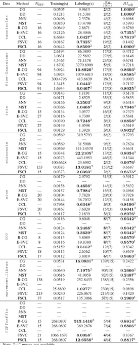
In Table III, we include SVC training time, cluster labeling time, the number of SEVs, the number of clus-ters and RIadj achieved by the evaluated algorithms separately. Rank of each item highlighted by boldface with superscript is given depending on its performance followed by corresponding rank (from 1 to 3).

In terms of ARI measure, except for wisconsion and zoo, FSCL achieves the best performance. More than this, it always reaches the first three rank in each evaluation

TABLE III.: Benchmark results on benchmark datasets.

Data Method NSEV Training(s) Labeling(s) (NNRC) RIadj

twocircles

CG — 0.0505 9.9613 2/(2) 1.00001

DD — 0.1213 11.5381 2/(2) 1.00001

kNN — 0.0496 2.3376 4/(2) 0.6968

MST — 0.0850 17.4798 8/(2) 0.5993

R-CG 16 0.0649 2.8671 4/(2) 0.6769

E-SVC 16 0.2126 28.4046 4/(2) 0.73553

CCL — 8.6684 1.04273 2/(2) 0.76192

FSVC 16 0.0167 0.73251 _{19/(2) 0.1402}

FSCL 16 0.0442 0.85992 _{2/(2) 1.0000}1

five-Gaussians

CG — 2.6194 86.3893 17/(5) 0.4712

DD — 3.0631 22.5692 27/(5) 0.6148

kNN — 4.5465 71.1178 23/(5) 0.6781 MST — 1.8702 3279.6909 5/(5) 0.7218 R-CG 94 3.0924 10.89263 _{17/(5) 0.8693}1

E-SVC 94 3.0924 1079.6013 18/(5) 0.85852

CCL — 300.4796 413.6639 19(5) 0.0003 FSVC 94 1.3415 1.04431 _{17/(5) 0.7137}

FSCL 91 1.6934 6.04672 _{17/(5) 0.8035}3

iris

CG — 0.0143 1.1191 11/(3) 0.6178

DD — 0.0171 2.8525 35/(3) 0.5833

kNN — 0.0156 0.35031 _{9/(3) 0.6414}

MST — 0.0366 1.04683 _{6/(3) 0.7946}3

R-CG 15 0.0134 3.0577 16/(3) 0.7373 E-SVC 27 0.0116 4.7309 2/(3) 0.5681 CCL — 0.0390 0.72482 _{3/(3) 0.8858}2

FSVC 27 0.0149 1.0598 5/(3) 0.5619

FSCL 15 0.0129 1.3928 3/(3) 0.90221

wisconsin

CG — 0.0569 319.5793 8/(2) 0.7793

DD — — — — —

kNN — 0.0569 31.5908 9/(2) 0.7624 MST — 0.0569 111.14570 11/(2) 0.6631 R-CG 15 0.0348 22.21053 _{13/(2) 0.8034}3

E-SVC 15 0.0373 443.1953 46/(2) 0.1344 CCL — 100.6628 23.6902 2/(2) 0.90761

FSVC 153 0.0383 13.01812 153/(2) 0.6687 FSCL 15 0.0373 2.03931 2/(2) 0.85752

wine

CG — 0.0179 2.9792 31/(3) 0.5912

DD — — — — —

kNN — 0.0158 0.46561 _{14/(3) 0.5632}

MST — 0.0157 0.79843 _{15/(3) 0.4968}

R-CG 20 0.0104 7.7820 20/(3) 0.7928 E-SVC 20 0.0144 36.7032 12/(3) 0.4158 CCL — 0.7968 0.63482 _{3/(3) 0.8190}2

FSVC 20 0.0167 7.6020 15/(3) 0.80413

FSCL 3 0.0117 2.1839 3/(3) 0.89761

zoo

CG — 0.0116 0.6048 8/(7) 0.93423

DD — — — — —

kNN — 0.0124 0.24881 _{8/(7) 0.9342}3

MST — 0.0124 0.36392 _{8/(7) 0.9342}3

R-CG 8 0.0113 3.8089 8/(7) 0.95701

E-SVC 8 0.0116 19.8380 8/(7) 0.95701

CCL — 0.5159 0.51523 _{12/(7) 0.8342}

FSVC 18 0.0115 2.6562 10/(7) 0.8679 FSCL 17 0.0112 3.8019 6/(7) 0.94632

movement

libras

CG — 0.0531 15.08313 139/(15) 0.2422

DD — — — — —

kNN — 0.0640 7.19752 _{90/(15) 0.2666}2

MST — 0.0616 41.0058 92/(15) 0.24873

R-CG 138 0.0519 252.8433 138/(15) 0.2356

E-SVC — — — — —

CCL — 25.8809 1.02771 _{230/(15) 0.0898}

FSVC 213 0.0240 226.0671 213/(15) 0.1420 FSCL 37 0.0517 135.3086 37/(15) 0.29691

P2PTraffic

CG — — — — —

DD — — — — —

kNN — — — — —

MST — — — — —

R-CG 15 268.0807 313.14163 _{5/(4) 0.8814}2

E-SVC 15 268.0807 369.2676 7/(4) 0.88053

CCL — — — — —

FSVC 21 1066.1697 8.00581 _{4/(4) 0.8367}

FSCL 15 268.0807 12.65562 _{4/(4) 0.8817}1

2.3483 2.5067

6.75 1.8497

2.6207

6.2667 5.3333 3.5238

1.2111

3.3797

1.7039 2.36

6 1.6695

1.5274

4.7333 4.5556 2.7143

1.1003

2.9114

sunflowers orange twocircles five-Gaussians iris wisconsin wine zoo movement_libras P2PTraffic

0 1 2 3 4 5 6 7

D

a

t

a

s

e

t

Average of the sample rate

FSCL

CG

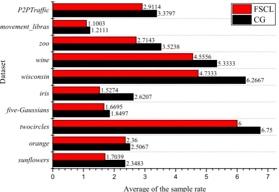
Figure 2: Comparison of the sample rate between CG and FSCL.

whereas performance of the others are unstable. In most cases,kNN, CCL and FSVC perform well, but the cluster labeling time increases dramatically as the dimensionality and size of a data set increases. Especially for FSVC, due to the drawback of preprocess which is similar to k−means [36], [37], it suffers from instabilities. An-other time-consuming algorithm is E-SVC, which fails in handling the 90-dimensional dataset movement libras. Notice that DD can hardly clusters such high-dimensional data since it can not construct the graph; therefore, it is only recommended to deal with low-dimensional data. For time consumption, SVC training and labeling are considered separately. In the view of methodology, CCL requires strict constraints to guarantee R ≤ 1 so that it frequently consumes much more time in SVC training; whereas the others cost similarly. In labeling phase, FSCL is consistently included in the first three ranks in most cases. Intuitively, an effective algorithm is expected to achieve a high accuracy with a corresponding number of clusters close to the exact number of classes. In table III, the NR denotes the number of clusters got by these algorithms while the NC is the exact number of classes summarized in table II. The highlighted NR by boldface

which is closest toNCalso suggests that FSCL is suitable

for exploring the distribution structure of a data set. To verify if the proposed sampling strategy reduces the sample rate m required by finding the connected components, we illustrate the average sample rate required by the FSCL and CG like algorithms respectively in Fig.2. Obviously, the significantly reduced average sample rates proves the effectiveness of the proposed strategy.

IV. CONCLUSION

In this paper, a novel fast and stable cluster labeling algorithm, namely FSCL is proposed to improve efficien-cy and accuraefficien-cy while keeps stability. Differing from the traditional cluster labeling algorithms, we consider to im-prove the accuracy as well as to reduce the time complex-ity by decreasing both the number of sampled point pairs

and the sample rate. We find that the SVs are sufficient to profile the cluster boundaries. Such that taking all of the data points to locate the SEVs is completely unnecessary and time consuming. Furthermore, while a reduced set of SEVs integrated from the SVs are obtained, the cost for finding connected components is significantly reduced. Meanwhile, in this study, we also confirm that the linear sample sequence generated by tradition algorithms would bring a quantity of redundant segmers to connectivity analysis. Therefore a disconnection checking first strategy is presented to achieve further improvement on efficiency. Even though a cluster might have multiple components to support irregular shapes, one component with one SEV is unable to handling imbalanced distributed data points well. Consider this problem, the density centroid is constructed by each subset of SVs with respect to a component; then two points used as prototype for a com-ponent in logical contribute to improvements on accuracy remarkably. Since no instable factor is brought in, the proposed FSCL algorithm is suggested to be fast and stable in comparison of the state-of-the-art algorithms.

Since the number of SVs would be one of the major factors related to efficiency, a more efficient strategy which can control the size of SVs while avoid unnecessary analysis with all of the data points is required to be further integrated.

ACKNOWLEDGMENT

The authors are grateful to the anonymous referees for their valuable comments and suggestions to improve the presentation of this paper.

REFERENCES

[1] R. Xu and D. C. Wunsch, Clustering. Hoboken, New

Jersey: A John Wiley&Sons, 2008.

[3] A. Ben-Hur, D. Horn, and H. T. Siegelmann, “A support vector cluster method,” inProceedings of 15th Internation-al Conference on Pattern Recognition, 2000, pp. 724–727. [4] A. BenHur, D. Horn, and H. T. Siegelmann, “Support vector clustering,”Journal of Machine Learning Research, vol. 2, no. 12, pp. 125–137, 2001.

[5] B. Scholkopf, J. C. Platt, and J. Shawe-Taylor, “Estimating the support of a high-dimensional distribution,” Neural Computation, vol. 13, no. 7, pp. 1443–1472, 2001. [6] D. M. J. Tax and R. P. W. Duin, “Support vector

do-main description,”Pattern Recognition Letters, vol. 11-13, no. 20, pp. 1191–1199, 1999.

[7] P. Ling, X. S. Rong, X. Y. You, and M. Xu, “Novel three-phase clustering based on support vector technique,” Journal of Software, vol. 8, no. 4, pp. 955–962, 2013. [8] C. Burges, “A tutorial on support vector machines for

pattern recognition,” Pattern Recognition Letters, vol. 2, no. 2, pp. 121–167, 1998.

[9] B. E. Boser, G. I., and V. Vapnik, “A training algorithm for optimal margin classifier,” inProceedings of the 5th annual ACM workshop on Computational Learning Theory, 1992, pp. 144–152.

[10] C. H. Guo and F. Li, “An improved algorithm for support vector clustering based on maximum entropy principle and kernel matrix,”Expert Systems with Applications, vol. 38, no. 7, pp. 8138–8143, 2011.

[11] P. Ling, C.-G. Zhou, and X. Zhou, “Improved support vector clustering,” Engineering Applications of Artificial Intelligence, vol. 23, no. 4, pp. 552–559, 2010.

[12] J.-S. Wang and J.-C. Chiang, “An efficient data prepro-cessing procedure for support vector clustering,”Journal of Universal Computer Science, vol. 15, no. 4, pp. 705– 721, 2009.

[13] Y. Ping, Y. J. Zhou, and Y. X. Yang, “A novel scheme for accelerating support vector clustering,”Computing and Informatics, vol. 31, no. 3, pp. 613–638, 2012.

[14] J. H. Yang, V. Estivill-Castro, and S. K. Chalup, “Support vector clustering through proximity graph modeling,” in Proceedings of the 9th International Conference on Neural Information Processing (ICONIP’02), 2002, pp. 898–903. [15] V. Estivill-Castro and I. Lee, “Amoeba: Hierarchical clus-tering based on spatial proximity using delaunay diagram,” in Proc. of the 9th Int. Symposium on Spatial Data Handling, 2000, pp. 7a.26–7a.41.

[16] V. Estivill-Castro, I. Lee, and A. T. Murray, “Criteria on proximity graphs for boundary extraction and spatial clus-tering,” inProceedings of the 5th Pacific-Asia Conference on Knowledge Discovery and Data Mining (PAKDD’01), 2001, pp. 348–357.

[17] T. Ban and S. Abe, “Spatially chunking support vector clustering algorithm,” inProceedings of International Joint Conference on Neural Networks, 2004, pp. 413–418. [18] W. J. Puma-Villanueva, G. B. Bezerra, and C. A. M. Lima,

“Improving support vector clustering with ensembles,” in Proceedings of International Joint Conference on Neural Networks, 2005, pp. 13–15.

[19] J. H. Chiang and P. Y. Hao, “A new kernel-based fuzzy clustering approach: Support vector clustering with cell growing,” IEEE Transactions on Fuzzy Systems, vol. 11, no. 4, pp. 518–527, 2003.

[20] S.-H. Lee and K. M. Daniels, “Cone cluster labeling for support vector clustering,” in Proceedings of 6th SIAM Conference on Data Mining, 2006, pp. 484–488. [21] ——, Gaussian Kernel Width Selection and Fast Cluster

Labeling for Support Vector Clustering. Technical Report, No. 2005-009, 2005.

[22] J. Lee and D. Lee, “An improved cluster labeling method for support vector clustering,”IEEE Transactions on Pat-tern Analysis and Machine Intelligence, vol. 27, no. 3, pp. 461–464, 2005.

[23] ——, “Dynamic characterization of cluster structures for robust and inductive support vector clustering,” IEEE Transactions on Pattern Analysis and Machine Intelli-gence, vol. 28, no. 11, pp. 1869–1874, 2006.

[24] D. Lee and J. Lee, “Equilibrium-based support vector machine for semisupervised classification,” IEEE Trans-actions on Neural Networks, vol. 18, no. 2, pp. 578–583, 2007.

[25] C.-H. Lee and H.-C. Yang, “Construction of supervised and unsupervised learning systems for multilingual text categorization,” Expert Systems with Applications, vol. 2-1, no. 36, pp. 2400–2410, 2009.

[26] D. Lee and J. Lee, “Dynamic dissimilarity measure for support-based clustering,” IEEE Transactions on Knowl-edge and Data Engineering, vol. 22, no. 6, pp. 900–905, 2010.

[27] D. Lee, K.-H. Jung, and J. Lee, “Constructing sparse kernel machines using attractors,”IEEE Transactions on Pattern Analysis and Machine Intelligence, vol. 20, no. 4, pp. 721– 729, 2009.

[28] K.-H. Jung, D. Lee, and J. Lee, “Fast support-based clus-tering method for large-scale problems,”Pattern Recogni-tion, vol. 43, no. 5, pp. 1975–1983, 2010.

[29] J.-H. Jung, N. Kim, and J. Lee, “Dynamic pattern denois-ing method usdenois-ing multi-basin system with kernels,”Pattern Recognition, vol. 44, no. 8, pp. 1698–1707, 2011. [30] L. Z. Peng, B. Yang, and Y. H. Chen, “Data gravitation

based classification,”Information Sciences, vol. 179, no. 6, pp. 809–819, 2009.

[31] H. C. Kim and J. Lee, “Clustering based on gaussian processes,”Neural Computation, vol. 19, no. 11, pp. 3088– 3107, 2007.

[32] F. Camastra and A. Verri, “A novel kernel method for clustering,” IEEE Transactions on Pattern Analysis and Machine Intelligence, vol. 27, no. 5, pp. 801–805, 2005. [33] A. Frank and A. Asuncion, “UCI machine learning

repository,” University of California, Irvine, School of Information and Computer Sciences, 2010. [Online]. Available: http://archive.ics.uci.edu/ml

[34] J. F. Peng, Y. J. Zhou, C. Wang, Y. X. Yang, and Y. Ping, “Early tcp traffic classification,” Journal of Ap-plied Sciences-Electronics and Information Engineering, vol. 29, no. 1, pp. 73–77, 2011.

[35] S. Sun and Y. Z. Wang, “Research and application of an improved support vector clustering algorithm on anomaly detection,”Journal of Software, vol. 5, no. 3, pp. 328–335, 2010.

[36] T. D. Hocking, A. Joulin, F. Bach, and J.-P. Vert, “Clus-terpath: an algorithm for clustering using convex fusion penalties,” inProceedings of the 28th International Confer-ence on Machine Learning (ICML), Bellevue, WA, USA, 2011, pp. 1–8.

[37] O. Shamir and N. Tishby, “Stability and model selection in k-means clustering,”Machine Learning, vol. 81, no. 1, pp. 213–243, 2010.