The Improvements for Extraction of Medical
Target Tissue Based on MC Algorithm
Xuemei Huang
Shandong University of Technology, Zibo, China Email: [email protected]
Weihong Liu and Hongquan Wang
Shandong University of Technology, Zibo, ChinaEmail: {chnlwh, whq2008}@sdut.edu.cn
Abstract—Computing redundancy, bad expansibility and “scalelike effect” lie in standard MC algorithm now. Furthermore, because of the complex structures in the segmented object, the triangular mesh model contains many isolated fragments. Fragments exaggerate the data size of the surface model and hinder the RP manufacturing speed. To solve the repeating calculation redundant problem, a suitable data structure was applied to seek cubes. By making segmentation result as the input of MC algorithm, the author eliminated the limitation of expansibility. By smoothing the normal vector of isosurfaces, this paper improved the image displaying effect. Finally, a special storage data structure was designed to save the non-manifold triangle model obtained from MC algorithm and a new defragmentation algorithm was presented to delete the corresponding triangle meshes whose computed volume were less than given threshold. The modification mentioned above has been realized in 3D reconstructing software-MedLG which was developed by authors’ institute and applied successfully in customized prostheses designing already.
Index Terms—medical target tissue, MC algorithm, isosurface
I. INTRODUCTION
MC algorithm is a classical 3D reconstruction method of medical image [1]. MC algorithm makes use of the Characteristics of the medical data adequately when it is applied to reconstruct the medical image and the high quality 3D images can be obtained by interpolating process. However, the realization of MC algorithm has some difficulties. In fact, MC algorithm obtained the high quality image by adding computing works and storage space [2]. The standard MC algorithm has the following four problems:
(1)The first is memory space and computing redundancy. The amount of medical data is very large. For example, a reconstructed pelvis image needs about 20M storage space. For more data, the memory can not
bear. Furthermore, the standard MC algorithm needs to deal with every cube in turn, but according to the statistic, the cubes intersecting with isosurface account for only ten percent of all cubes [3]. Much time has been used to detect the blank cubes, which cause repeating calculation and the resources of computer are wasted. Moreover, the computing error can be induced by repeating calculation of floating point. So a suitable data structure is needed to seek cubes.
(2) The second is bad expansibility. The standard MC algorithm can extract the isosurface by thresholding segmentation method [4], for example, according to a certain CT value. The expansibility of MC algorithm thus is limited. If many kinds of segmentation method can be integrated in MC, the expansibility of MC will be improved greatly.
(3) The third is definition of display. The 3D image reconstructed by the standard MC algorithm is not very clear. For a cube, the location and orientation of triangles in it are interfered easily by noise, which can cause “scalelike effect” in displaying [5, 6].
(4) The last is fragments problem. The triangle model of target tissue extracted by MC algorithm is a non-manifold model because of the floating point operation error and the existing of cancellous bone. The triangle mesh model contained many isolated fragments. However, Fragments exaggerated the data size of surface model and lower the RP manufacturing speed.
II. THE IMPROVEMENT OF MC ALGORITHM The medical data are composed of sectional data files. The author realized the improvements of MC algorithm according to the characteristics of medical data integrating Cuberrille algorithm at the same time [7]. A. Data Extraction of DCM File
Firstly we needed to extract the pixel information from the DICOM images file and then extracted the interested tissue by image segmentation.
It was necessary to simplify the information of DICOM image files, extracted the major and removed redundant information.
Generally, the information of DICOM data is uniquely determined by the data element tag. Firstly we found the corresponding labels when checking the required data information, then read out the data content in the data elements. Data element tag is constituted by the group number and data element number. We could find the corresponding group numbers, and then judged the information corresponding to the data elements number. The group numbers concerned with pixel values and image information are 0028, 0020 and 7EF0.
For example, we needed to extra the image pixel data. Firstly found the data elements which group number was 7EF0, and then found the data elements that express pixel data values, whose data element number is 0010.The data contained in data elements was the value of the pixels, then extracted pixel values according to the structure of data elements.
The specific content could be found in the DICOM standards [8-10]. The flow chart of DCM extraction was shown in Fig.1.
B. Eliminating Memory Space Occupation and Computation Redundancy
The medical data can be stored in octree or three-dimensional array. Octree storage can seek the data more quickly than three-dimensional array.
For MC algorithm, it must use the information of adjacent cubes when dealing with one cube. The treating way is one section by one section. However, octree stores the cube data with tree form structure which all needed to be read in memory one time. The occupation of memory space is large and difficult to compress as well. In addition, octree has complicated implementing process, which cause sectional segmentation and treating difficulties.
Considering the factors mentioned above, the author still used the three-dimensional array. To save the memory space, the improved algorithm dealt with data along the X and Y scanning direction in turn. Because the treating of one cube needs six cubes of X, Y and Z directions, the algorithm only stored the data of four slices in memory one time. After finishing the data of one layer, the algorithm would read the data of four new slices. By establishing such exchanging mechanism, the system held down the requirement of memory space greatly. The occupation of memory space related to the resolution of slice but not the quantity of slices.
By analyzing we know that if the isosurfaces intersecting with a cube (for example, CubeA) was determined, then the isosurfaces would extend in the neighbors of CubeA. In this paper, we added a flag to the fifteen basic structure of MC algorithm. The flag recorded the number of the visited cubes of the six neighboring cubes. For the six neighbors, the number of the visited might be 0, 3, 4, 5, and 6. For example, we sought only the three neighbors of a cube in Case-3 in [1], but we needed seek all six neighbors of a cube in Case-10 in [1]. According to our statistic, 90 percent of isosurfaces were composed by the six cases showed in Fig.2. Thus a lookup table could be set to record the information of neighbors for every basic structure of MC algorithm and a queue could be introduced to record the cubes treated already at the same time. A great of time could be saved through above modification to MC.
To reduce the calculating further, this paper fully utilized the characteristic of medical structural data. Every vertex (for example, VertexA) of a cube was shared by four cubes which share a same edge, so every cube could be treated along X, Y, Z direction in turn. Namely only the vertex of three edges were needed to calculate by interpolating and the vertexes of triangles lying on the rest nine edges could be obtained from the
Figure2. Cube tracking N
If “DCM” format?
Find the group number of Data Element Tag corresponding to patient
information, pixel information, etc.
Read pixel data Y
End Start
Find data element number of Pixel parameters and pixel value in the group
number have found
previous calculation. The author utilized such calculating relativity. When a new vertex was calculated, the result was sent to the corresponding location of next untreated cubes which share the same vertex. The buffer should be reserved for the current layer and the next layer to be dealt with in memory.
As shown in Fig.3, when calculating the point of intersection e4, we needed to send the calculating result to
data buffer area of corresponding intersecting points of neighbor cubes which share e4, for example the
intersecting points of e5, e6, e7.
Accoring to the modification mentioned above, the basic data structure needed another lookup table NBCase and structure lookup tale TA[i][j] to record the information of neighbor cubes for every structure form, a queue QCube to record the treated cubes and a dualistic flag array M={Flag, C} to reflect the visited information of cubes except structure index table VIndex.
When starting, M was initialized and all elements were set to zero. Then a seed cube was selected (a cube that intersecting with isosurface) and put in the QCube. The flag value was set to 1. Every time a cube was taken out from QCube, two judges must be needed: one was the structure form of the cube. Then the intersecting point and normal vectors would be calculated and added to triangle arrays TRA. The other is which neighbors would be visited determined by NBCase and added that neighbor cube to QCube. By the above processing, a seed cube was thought to finish Traversal. The algorithm would keep on running until QCube is blank. Finally, the extraction of isosurface was over and the reconstructed triangle model could be displayed.
The flow of Modified algorithm was as following: IN: the 3D data set
OUT: the triangle array TRA
(1)Read the lookup table of intersecting point of edge EIndex and structure form lookup tale TA[i][j];
(2) Initialized M, set the Flag value of all elements 0 and set QCube blank;
(3) Detected data set and selectd a cube Cube1 whose structure form was not zero. Looked up NBCase by VIndex of Cube1 and putted the neighbor cubes sharing the common intersecting point with Cube1 into Qcube, circulate step (3) to (5);
(4)Calculated the VIndex value of cubes and according to VIndex value found the edge intersecting with isosufaces from EIndex;
(5)Calculated the coordinate of intersecting point; (6)Looked up TA[i][j] according to VIndex, determined the connecting turn of triangle;
(7)Outputted the triangle array TRA.
C. Enhancing the Expansibility of MC Algorithm (1) The segmentation method used in this paper
Threshold segmentation is a commonly used image segmentation technology in medical images. The basic principle is as follows: It divided image pixels into two or more independent class through setting different characteristics threshold. Such segmentation algorithm can divide various tissues from background effectively. However it involved in the problem of more threshold choosing in image processing. The main shortcoming of the algorithm is that the search space is too large and the convergence rate is too slow [11].
Seeded region growing algorithm is a region-based semi-automatic segmentation algorithm. The algorithm has highly response speed and reliable function, which is suitable for segmentation of various images. The seed needs to choose manually. A single regional growth starts from a seed pixel; search all adjacent neighbors of seed pixel. If elements of segmentation matrix corresponding to adjacent neighbors are 1, identifies it as 2. Then, search recursively for all adjacent neighbors, until you can not find element “1” corresponding to adjacent neighbors. The seeded neighbor region is regular polygon, which has 18-neighbors or 26-neighbors [12].
This paper adopted an algorithm integrating the threshold segmentation with seeded region growing segmentation. Firstly, set a threshold according to the CT number of target tissue, identified the elements within the setting threshold with monochrom which was diffident from the original grayscale image. Observed the segmentation result, re-adjusted the threshold if needed. Then initialized the segmentation matrix and selected a seed in target tissue region. Next set the seed as the starting point to execute the seeded region growing operation and identified the segmentation result with another monochrom. Last, observed the segmentation result and repeated the above process if the result was not ideal.
Neighbor region with 26 neighborhood pixels was adopted. Fig.4 was the illustration of 26 neighborhood pixels; each point represented a pixel, represented the seeded pixel.
Usually, the target tissue accounted for a small part of whole image. The segmentation matrix was sparse and the storage space could be reduced further by octree coding or sparse matrix coding. However, the system needed to code or decode for every random accessing, which affect the segmentation speed. It often needed to reset the threshold and the location of seed when segmented the target tissue in practice. So the further space reducing must be reconsidered to prevent the low segmentation speed. Moreover, even though not considering the compressing further, the algorithm must
v0 v
1
v2 v3
v0 v
1
v2 v3
v4 v5 v4 v5
v6 v6
v7 v7
e2
e0 e1 e3
e5 e4
e6 e7
e8 e9 e10
e11
be designed to reduce time complexity of random accessing and matrix initializing.
Fig. 5 was the seeded region growing algorithm.
The number of rows and columns is the multiple of 4. According to the row or the column, every four pixels of segmentation result could be combined to a byte. The segmentation matrix was shown in Fig.6.
According to Fig.6, layers and rows were kept changeless and columns were reduced to a quarter of original number. The operation to the segmentation matrix mainly included the following case: the initialization of segmentation matrix; the random accessing in segmenting process; the computation of isosurface and reading the segmenting result when extracting the contour in later steps.
The random accessing in segmenting process mainly included the shift of single byte, AND operation and OR operation. The speed of bitwise operation was very fast, which has little affection to the time complexity of segmenting operation. So the initialization of segmentation matrix and reading the segmenting result by
layer should be paid more attention. Every byte of segmentation matrix corresponded to four pixels, so when initializing, a byte should be filled before the next writing. For the reading the segmenting result by layer, the shift operation to extract the four segmenting result should be executed when reading a byte every time.
(2) Inputing the Segmenting Result for MC
To throw away the limitation of thresholding segmentation, the segmenting result could be inputted to MC. Thus the most suitable method was selected according to the feature of an image and the isosurfaces could be formed by segmenting result. Of course, the segmenting result was a binary image by this way.
When calculating the point of intersection of the isosurface with a cube, there were no suitable thresholds to finish interpolating calculation because of binarization. The author directly selected the midpoint of edges of a cube as the point of intersection of the isosurface with a cube, which could omit the calculation of linear interpolating. The maximum error was a half cube if the midpoint was used to represent intersecting point. However the resolution of ordinary display could not reach this definition. For a 512×512 data set, the screen image projected by midpoint almost had the same displaying effect comparing to the image projected by point obtained from linear interpolating.
Many segmenting algorithm could be integrated with MC algorithm if the segmenting result was inputted to MC. The modularity and expansibility could be improved correspondingly.
Fig. 7 showed the 2D display of the extraction to skull tissue of the patient applying the segmenting algorithm mentioned above.
D. Smoothing of Isosurfaces
To obtain the clear reconstructing result and get rid of “scalelike effect”, this paper dealt with the direction of isosurfaces.
Assuming the isosurfaces obtained from MC algorithm was:F0={( ti, Ni ) | i=0,1, …, N}.
N was the total number of triangles. Ni was the unit normal vector of one triangle ti. For ti, the unit normal vector was:
Figure 4. Illustration of 26-neighbors
Figure 6. Segmentation matrix //Q is a queue to store the identified region
elements, Seed is the seeded pixel Label(seed)=2;
PushSeed into Q;
x[9]={0,1,1,-1,-1,-1,0,1}; y[9]={0,0,1,1,1,0,-1,-1,-1}; While(Q is not empty)
{
NewSeed=Remove(Q); for(z=-1;z<=1;z++)
for(i=0;i <9;i ++) {
Neighbor=NewSeed +((x[i],y[i],z); if(Element(Neighbor)==1) {
Label(Neighbor)=2; PushNeighbor into Q; }
} }
) ( ) (
) ( ) (
i k i j
i k i j
v v v v
v v v v
N
(1)
According to illumination model of rendering in 3D graphics library, we knew that the 3D displaying effect of triangle ti was related to the direction of the normal vector of ti. We assumed that the set of neighbor triangles of ti was {t1, t2, …, tk}, the corresponding normal vectors were Nt1, Nt2,…, Ntn, then the average value could be obtained:
) (
) (
) (
) (
1 1
1 1
0 0 '
mi mk mi mj
mi mk mi mj n
m n
m ti t
v v v v
v v v v n
N n
N
(2)
The value of Nt’ was then assigned to Nt. We could get the smoothed vector field of isosurfaces by dealing with all normal vectors of triangles in this way. The reconstructed image looks clearer accordingly. The Fig.8 showed the comparative effect of non-smoothed and smoothed.
D. The Storage Data Stuacture Of Non-uniform Triangle Model
When MC algorithm was used to extract isosurface to display the medical image data, usually a non-manifold triangle model was produced.
For the non-manifold triangle model storage, the simplest method is to use vertexes list and triangle faces list. The vertexes list has the coordinate information of
vertexes and the faces list has the pointers to vertexes. Because the non-manifold triangle model might have the isolated vertexes and isolated edges, a table was needed to record the linking relation of vertexes. The linking relation table of vertex is a 2D matrix applied widely in graph theory. If the number of vertex of a grid model is n, then 2D matrix n×n is sparse of course. Only has linking relation were two vertexes set to 1, the rest were set to 0. Applying the vertex linking matrix could cause the waste of storage space and the low efficiency of looking up.
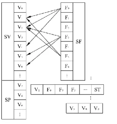
In this paper, a list ST of vertex and face was adopted to take the place of the vertex linking matrix. An index of vertexes was put ahead of faces list. Then a list SE of isolated edges was established. ST, SE, vertex list (include vertexes of face SV and isolated vertexes SP) and triangle face list SF were applied together to store the non-manifold triangle model. The Fig.9 was the storage structure of non-manifold triangle model.
F. Defragmentation Process
Because of the floating point operation error in isosurface extraction and the existing of cancellous bone, the triangle mesh model contained many isolated fragments shown in Fig.10.
Fragments exaggerated the data size of surface model and hinder the RP manufacturing speed. Thus Defragmentation algorithm was presented in this paper. Usually the fragments were the closed the triangle mesh
(a)Non-smoothed (b) smoothed
Figure 8. the comparative effect of non-smoothed and smoothed
Figure 10. The isolated fragments
with small volume. The idea of algorithm was to find all the isolated spanning trees after isosurface extraction process, and then computed the volume of every spanning tree or the volume of circumscribed cuboids to decide the deleting single isolated spanning trees or not according to the value of volume.
(1)The computation of the volume of tetrahedron Assuming the tetrahedron T showed in Fig.11 (a) was composed of four vertexes a( v1a, v2a, v3a), b( v1b, v2b, v3b), c( v1c, v2c, v3c) and d ( v1d, v2d, v3d).
The formula of volume of V(T) was:
1 1 1 1
6 1 ) (
3 2 1
3 2 1
3 2 1
3 2 1
d d d
c c c
b b b
a a a
v v v
v v v
v v v
v v v T
V (3)
V(T) was a signed value in the above equation. For example, when the observing direction was opposite to the outer normal of triangle made up of a, b, c and the connecting order of a, band c was anticlockwise, then the value of V(T) was positive and the opposite was the other way around. In Fig.11(b), the coordinates of the four vertexes of the tetrahedron were : a(1,0,0), b(0,1, 0), c(0,0,1), d(0,0,0). According to (3), V(T)=1/6.
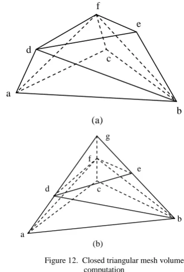
(2) The computation of the volume of closed triangle mesh
To deduce the computation formula of closed triangle mesh, considered a simple closed mesh abcdef composed of eight triangles in Fig.12 (a). All the outer normal of triangles pointed to the outer of mesh. Prolonged the edges ad, be and cf to a point g. The Fig.12 (b) showed
that the volume of tetrahedron abcg composed of vertex g and underface abc was positive and the volume of tetrahedron defg composed of vertex g and face def was negative. Other volume of tetrahedrons composed of vertex g and the rest six faces was zero. So the volume of mesh V(abcdef) equaled to V(abcg)+V(defg). In fact, the volume of mesh V(abcdef) was the algebraic volume sum of eight tetrahedrons composed of vertex g and eight triangles. Though the vertex g in Fig.12 (b) had a special position and the conclusion was obvious. It is not difficult to prove that for vertex with any position, the conclusion mentioned above is tenable. For any close triangle mesh M and any vertex g, the volume of triangle mesh M is:
M f
v v v f f g f
V M
V( ) ( 1 2 3 ) (4)
Where: fv1, fv2, fv3 are the three vertexes of triangle f. The connecting order of fv1, fv2, fv3 is determined by the normal direction of f and right-handed screw rule.
(3) Defragmentation algorithm
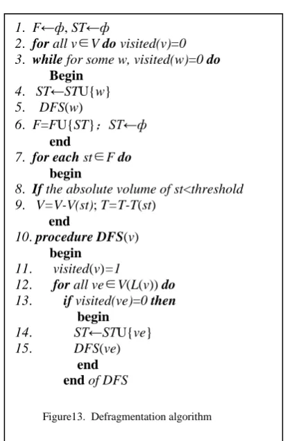
Assuming the triangle model after extracting was M=(V,T).Usually M included one or more close triangle meshes. V was the set of all vertexes and T was the set of all triangle faces. For every vertex v∈V, constructed a link list L(v) and added all the vertexes in L(v).
Firstly, traversing depth-first all the vertexes to find all the isolated spanning trees, the forest F={ STi } would be formed . Next, for every spanning tree st∈F, computed the volume of st. If the absolute value volume was less than the setting threshold according to (4), deleted all the vertexes V(st) and all the triangle face F(st) composed of V(st) in spanning tree st. The setting threshold should satisfy that deleted the fragments with small volume but (a)
a
b d
c
a
b c
d
X
Y Ⅰ
Ⅰ
Ⅰ
(b) Z
Figure 11. Tetrahedron volume computation
(a) a
b c
d
e f
a
b c
d
e f
g
(b)
not including the important faces. Assuming the vertexes set V(L(v)) was a point set which lied on the same edge to vertex v in L(v),the algorithm was shown in Fig.13.
A 3D reconstructing software MedLG including improved MC algorithm developed by ourselves was used to design an ear prosthese for a patient with a missing ear in Fig.14. In Fig.14(c), the model in left image was manufactured by LOM (Laminated Object Manufacturing) technics[13].
Ш.CONCLUSIONS
The improved method proposed above can eliminate the memory space occupation and computing redundancy effectively, and expand the commonality of standard MC algorithm. At the same time, by adjusting the direction of isosurface, the “scalelike effect” can be weaken to some extent and the image obtained has better displaying effect.
Because the grid model extracted by MC algorithm is non-manifold, the storage data structure adapting to non-manifold triangle model is presented in this work. Especially, a defragmentation algorithm is put forward to delete the useless information, thus the data of the reconstructed model and the later RP manufacturing time can be reduced.
ACKNOWLEDGMENT
The authors wish to thank Min Ye, Chengtao Wang for their generous support of this research. In particular, the RP models were completed in KINEGRY Company in Shanghai. The authors wish to acknowledge with thanks the help of staff in the company in producing the RP models through the use of their facilities.
REFERENCES
[1] W. Lorensen, H. Cline, “Marching cubes: A high resolution 3D surface construction algorithm”, Computer Graphics. 1987, 21(3): pp.163-169.
[2] A. Gelder, J. Wilhelms, “Topological considerations in isosurface generation”, ACM Trans. On Graphics, 1994, 13(4): 337-375.
[3] J. Wilhelms, A. VanGelder, “Topological considerations in isosurface generation”, San Diego Workshop on Volume Visualization, 1990, 24(5): pp.79-86.
[4] R. Adams, L. Bischof. “Seeded region growing”, IEEE Trans. on Pattern Analysis and Machine. Intelligence, 1994, 16(6): pp.641-647.
[5] C. Xu, D. Pham, “Rettmann M E, etal. Reconstruction of the human cerebral cortex from MRI”, IEEE Trans .on Medical Imaging, 1999,18(6): pp.467-479
[6] J. Chen, H. Wechsler, “Knee surgery assistance: patient model construction, motion simulation, and biomechanical visualization”, IEEE Trans. on Medical Imaging.2001, 48(9): pp.1042-1052
[7] S. Shephard, K. Georges, “Automatic three-dimensional mesh generation by the finite octree technique”,
International Journal for Numerical Methods in Engineering, 1991, 32: pp.709-749.
[8] Digital Imaging and Communications in Medicine (DICOM) Based Standard. National Electrical
Manufacturers Association,
ftp://medical.nema.org/medical/dicom.
[9] C. S. Xie, “Research and Implementation of DICOM Image Displaying”, Computer Engineering & Science, 2002, 24 (6), pp. 38-42.
[10]H. Y. Quan, “DICOM data sets and DCM file format”,
Computer Application, 2001, 21 (8), pp. 145-148.
[11]D. J.Wu, “New medical image segmentation algorithm based on subregion similarit”, Journal of Computer Application, 2010, 30(9), pp. 2458-2460.
[12]Y. X. Shi, “The medical image segmentation algorithm based on edge detection and regional growth”, Journal of Xi’an Polytechnic University, 2010, 24 (3), pp. 320-323.
(a)non-smoothed (b) smoothed
(c)the rapid prototyping modeland silicon ear
model
Figure 14. The appliation of improved algorithm on customized auricular prothese. 1. F←ф, ST←ф
2. for all v∈V do visited(v)=0 3. while for some w, visited(w)=0 do
Begin
4. ST←STU{w} 5. DFS(w)
6. F=FU{ST};ST←ф end
7. for each st∈F do
begin
8. If the absolute volume of st<threshold 9. V=V-V(st); T=T-T(st)
end
10.procedure DFS(v) begin
11. visited(v)=1
12. for all ve∈V(L(v)) do
13. if visited(ve)=0 then
begin
14. ST←STU{ve} 15. DFS(ve)
end end of DFS
[13]X. M. Huang, “Fabricating auricular prostheses based on rapid prototyping and the FreeForm modeling system”, The International Journal of Advanced Manufacturing technology, 2004, 24(11), pp. 873-878.
Xuemei Huang was born in Nanchong city, Sichuan province, China, on December 25, 1974. Xuemei Huang received her BS in Mechanical Design, Manufacturing and Automation from Shandong University, Shandong, China in 2001, and phD in Mechanical Design and Theory from Shanghai Jiaotong University, Shanghai, China. The main research field of Xuemei Huang is digital design and manufacturing.
She now worked in School of Mechanical Engineering, Shandong University of Technology. The main research articles include: “Fabricating auricular prostheses based on rapid prototyping and the FreeForm modeling system”, The International Journal of Advanced Manufacturing technology, 2004, 24(11), pp. 873-878. “Mesh generation from 3D scattered data in ACL surgical navigation system ”, First International Multi- Symposiums on Computer and Computational Sciences, IMSCCS'06, Shanghai, 2006,2:279-282. In past eight years, her research interest was digital clinic engineering.
Dr. Huang became a member of World Association of Science Engineering (WASE) in 2009.
Weihong Liu was born in Shandong province, China, on December 22, 1971. Weihong Liu received her BS in Mechanical Design, Manufacturing and Automation from Shandong University of Technology, Shandong, China in 2006. The main research field of Weihong Liu is digital design and manufacturing.
She now worked in School of Mechanical Engineering, Shandong University of Technology. The main research articles include: “Study on conceptual design and detail design of part based on 3d structure cell technology”, Zhongguo Jixie Gongcheng, 2006, 17 (22), pp.2346-2350.
Hongquan Wang was born in Shandong province, China, on July 7, 1975. Hongquan Wang received his BS in Mechanical Design, Manufacturing and Automation from Shandong University of Technology, Shandong, China in 2003. The main research field of Hongquan Wang is digital design and manufacturing.