Modified Particle Swarm Optimization Combined
with Trigonometric Function and Variable
Neighborhood Search
Wenxue Zhang
School of Science, Ningxia Medical University, Yinchuan 750004, China Email: [email protected]
Abstract—Based on the inertia weight and acceleration coefficients of trigonometric function and variable neighborhood search, a modified particle swarm optimization is discussed. The modified PSO with the parameters of the trigonometric function has powerful global exploration at the beginning and ending of the evolution, and strongly local exploitation in the interim of run. Through analyzing the behavior of the PSO, three novel heuristic neighborhood search rules are suggested to enhance the robustness and convergence. The proposed approach demonstrates its superiority in convergence, robustness and solution quality with the experiment tested on the benchmark multimodal function.
Index Terms—particle swarm optimization, trigonometric function, variable neighborhood search, inertia weight, acceleration coefficients
I. INTRODUCTION
The particle swarm optimization (PSO), inspired by social behavior of bird flocking and fish schooling, is a stochastic population-based powerful optimization technique for solving global optimization problems, firstly proposed by Kennedy and Eberhart [1,2]. PSO has many similarities with evolutionary computation techniques such as genetic algorithm (GA). However, unlike GA, PSO has no evolution operators such as crossover and mutation. The advantages of PSO are fewer memory requirement, shorter computational time and easy to implement. So it has gained popularity lately and has already been applied to different fields widely, such as function optimization, artificial neural network training, data mining, scheduling problem, pattern classification and fuzzy system control [3-5]. However, as many evolutionary algorithms, PSO does exhibit some disadvantages: it faces the problem of the appropriate parameters adjustment [6,7]; sometimes it is easy to trap in local optima and severely limited by the high computational cost of the slow convergence rate, especially in complex multimodal optimal problems [8-10].
Fortunately, many researchers are devoted to improve the performance of standard PSO and rich harvests have been obtained in three aspects.
Firstly, a few theoretical studies of particle trajectories can be found, which facilitated the derivation of
heuristics to select parameter values for guaranteed convergence to a stable point [11-12].
Secondly, many approaches and strategies are proposed to enhance the performance of PSO without sacrificing the speed of solution significantly by adjusting inertia weight and acceleration coefficients. Namely, there are linearly decreasing inertia weight, increasing inertia weight, randomized inertia weight, exponential decreasing inertia weight, fuzzy adaptive inertia weight, and linearly decreasing acceleration coefficients [7,8,13].
Finally, in order to improve the performance of PSO, various neighborhood search techniques are proposed to increase information sharing among the neighbor particles. Mohais [14] proposed a dynamically adjusted neighborhood. Janson [15] used dynamic hierarchy to define the neighborhood structure. Fan [9] addressed the method of combing PSO with a local simplex search technique. Liu [16] presented a center particle swarm optimization. Unlike other ordinary particles, the center particle has no explicit velocity, and is set to the center of the swarm at every iteration. Furthermore, hybridization of PSO with others evolutionary algorithms has been investigated in many studies [17,18].
In this paper, an improved particle swarm optimization is considered based on the inertia weight and acceleration coefficients of trigonometric function and variable neighborhood search, called TFVNS-PSO. This work differs from the existing ones at least in two aspects: firstly, it proposes the dynamic inertia weight and the dynamic acceleration coefficients that are the trigonometric functions of iterations, which change dynamically in accordance with sigmoid. Therefore, it has powerful global exploration at the beginning and ending of the evolution, and strongly local exploitation in the interim of run. Secondly, it presents several novel heuristic neighborhood search strategies to balance the convergence and diversity of particle swarm. Thus it overcomes premature convergence and improves the rate of convergence simultaneously.
II. STANDARD PARTICLE SWARM OPTIMIZATION
The standard PSO is proposed by Shi and Eberhart in 1998 [19]. Theoretically, given a d -dimension minimum
optimization problem f X( ), for the ith particle in the t th generation, letvid( ) [t ∈Vmin,Vmax], where Vmin and
max
V are constants depended on given problem; let
min max
( ) [ , ]
id
x t ∈ X X be the location of the particle, where min
X andXmax are the boundaries of the search space. The
location of the best fitness achieved so far by the ith
particle is denoted as pid( )t (memorized by every particle) and the index of the global best fitness by the whole population, as pgd( )t (memorized in a common repository). The velocity and position update equations are given as:
1
( 1) ( ) ( ( ) ( ))
id id id id
v t+ =ωv t +cξ p t −x t
2 ( gd( ) id( ))
cη p t x t
+ − (1)
( 1) ( 1) ( ), 1, 2,...,
id id id
x t+ =v t+ +x t i= m (2)
wheremis the population size; c1andc2, known as the
cognitive and social parameters respectively, are named acceleration coefficients; ξandη are elements from two uniform random sequences in the range [0,1] , namely,
, U(0,1) ξ η∈ .
The best positions are updated at every iteration step as follows:
( 1), ( ( 1)) ( ( )) ( 1)
( ),
i i i
i
i
X t if f X t f P t
P t
P t otherwise
+ + <
⎧
+ =⎨
⎩ (3)
In recent versions, the parameters are selected such that the relation [12-14],
1
1 2
2(c c ) 1
ω> + − (4)
where, 1− ≤ ≤ω 1 (5)
and 0≤ + ≤c1 c2 4 (6)
The procedure of PSO is given as follows:
Step1: Initialization
Step1.1t=0, (0)vi and (0)xi ;
Step1.2 Calculate (0)pi andpg(0);
Step2: While termination criteria is satisfied do
Step2.1 for i( =1;i<=m i; + +){ Update ( )v ti using (1);
Update ( )x ti using (2);
Update ( )p ti using (3);
if ( ( ( ))f p ti < f p t( g( ))) then p tg( )=p ti( );
} //end for Step2.2t= +t 1;
Step3: Output.
III. TFVNS-PSO
This section proposes the dynamic inertia weight and the dynamic acceleration coefficients that are the trigonometric functions of iterations, such that TFVNS-PSO has powerful global exploration at the beginning and
ending of the evolution, and strong local exploitation in the interim of run. In order to balance the convergence and diversity of particle swarm, several novel heuristic neighborhood search strategies are presented in following.
A. The inertia weight of trigonometric function (TFIW)
A vital issue of the intelligent optimization methods is to balance global exploration and local exploitation. Generally, in order to avoid trapping in local optimum at the very start, the coarse exploration is necessary in the initial iterations; in order to turn away sightless searching whole space, the stronger exploitation is required in the medium-term iterations; in order to jump out local optimum, the powerful exploration is the only way in later iterations.
As far as PSO goes, the balance between global exploration and local exploitation is achieved chiefly by adjusting inertia weight. A higher value of the inertia weight offers sharp changes in velocity, which means better exploration. However, smaller inertia weight implies less variation in velocity to provide better exploitation.
But the change trend of inertia weight is only in one direction and the decreasing direction is popular in the existing studies [7,8,13]. A novel inertia weight of trigonometric function (TFIW), therefore, is proposed to address this problem as follows:
' cos(t )
T
ω = π , (7)
' '
' '
ω ω α
ω
ω α ω α
⎧ ≥
⎪
=⎨
+ <
⎪⎩ (8)
where, T is a maximum number of iterations; t is a
iterative counter, t∈{0,1,..., }T ; α is a constant,
[0.1,0.4]
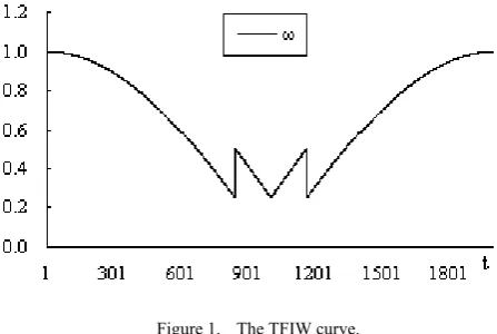
α ∈ , α =0.25 is proposed. The corresponding TFIW curve is depicted in Figure 1 for α =0.25 andT =2000.
Figure 1. The TFIW curve.
Farther, TFIW is a nonlinear function of the present iteration number t and maximum number Tof iterations.
B. The acceleration coefficients (c1 and c2) of trigonometric function (TFAC)
The higher value of cognitive parameter c1 and social
parameter c2 may provide powerful exploration and
strong exploitation, respectively [20]. Therefore, the higher c1 and smaller c2 must be satisfied in the initial
and later of the iterations, and the smaller c1 and higher
2
c must be satisfied in the middle of the iterations, which
should help the PSO to approach the optimum solution quickly. Consequently, this paper proposes the novel dynamic acceleration coefficients of trigonometric function for improved performance of PSO algorithm as follows:
' ' '
1
c = × ×b ω ω (9)
' '
1 1
1 ' '
1 1
c c
c
c c
β
β β
⎧ ≥
⎪
=⎨
+ <
⎪⎩ (10)
' '
2 1
c = −b c (11)
' '
2 2
2 ' '
2 2
c c
c
c c
γ
γ γ
⎧ ≥
⎪
=⎨
+ <
⎪⎩ (12)
where, b is a constant, b∈(0, 4), b=2 is proposed;
β is a constant, β∈[0.1,0.4], β =0.25 is proposed;γ is a constant, γ ∈[0.1,0.4] , γ =0.25 is proposed. The corresponding TFAC curves are depicted in Figure 2 for
2
b= ,α =0.25,β =0.25, γ =0.25and T =2000.
Figure 2. The TFAC curves.
Figure 3. The R curve.
Let, 1
1 2
2( ) 1
R= −ω c +c + (13)
The corresponding R curve is depicted in Figure 3
forb=2,α =0.25,β =0.25, γ =0.25 and T =2000.
Figure 3 shows the R curve withb=2,α =0.25,
0.25
β = , γ =0.25 , and T =2000, from which it’s clearly demonstrated that inequality (4) can be always satisfied with proposed dynamic parameter selection mechanism.
C. Variable neighborhood search
A neighborhood search algorithm typically starts from a solution (that is, an assignment of values to its decision variables) and moves from solutions to neighboring solutions in hope of improving a function f . The
function f measures the quality of solutions to the
problem at hand. The main operation of a neighborhood search algorithm amounts to moving from a solution s to
one of its neighbors. The set of neighboring solutions of
s, denoted by ( )N s , is called the neighborhood of s. At
a specific computation step, some of these neighbors may be legal, in which case they may be selected, or they may
be forbidden. Once the legal neighbors are identified (by
operationL), the local search selects one of them and
decides whether to move to this neighbor or to stay at
s(operationS). These concepts, which define the moves
in local search, are illustrated as follows [21].
The basic neighborhood search template
Function NeighborhoodSearch{ s:=GenerateInitalSolution();
;
s∗=s
for k=1 to MaxTrials do{
if satisfiable s( )∧f s( )< f s( )∗ then { s∗=s;} //end if ( ( ( ), ), );s=S L N s s s
}//end for Return s∗=s;
}//end function NeighborhoodSearch
Variable neighborhood search (VNS) is a recent metaheuristic for solving combinatorial and global optimization problems whose basic idea is systematic change of neighborhood both within a descent phase to find a local optimum and in a perturbation phase to get out of the corresponding valley [22]. Its development has been rapid, mainly to allow solution of large problem instances, such as highly-constrained nurse rostering problems, multi-resource generalized assignment problem, jobshop scheduling problems [23-25].
Definition 1: The set of neighborhood of the particle s , denoted byN s( ), is defined as
( ) { | s s s}
N s = s∗ x∗ =v∗+x , (14)
where, s s 1 ( s s) 2 ( s s)
gd
v∗ =ωv +cξ p −x +cη p −x and
min max
[ , ]
s
v∗∈V V .
Definition 2: The set of legal neighborhood of the particle s , denoted by ( ( ), )L N s s , is defined as
min max
( ( ), ) { | ( ) s [ , ]}
L N s s = s∗ s∗∈N s ∧x∗∈ X X .(15)
D. Heuristic neighborhood search for the original particle (HNSOP)
As one point of view, in order to improve the rate of convergence, when a new particle, denoteds, is created
randomly, ( ) ( )0
f s < f s (minimal optimization
function f , original particle s0 , s∈L N s( ( ), )0 s0 ) is
expected. As another point of view, in order to avoid premature convergence, a degrading particle is accepted with probability. To this addressed problem, a wholly new heuristic neighborhood search for the original particle (HNSOP) is proposed.
Definition 3: The set of neighborhood of the original particle, denoted byNOP( )s0 , is defined as
0 1 1 0
( ) { | ((i i ( ( i ), i ), ( )i ( ),
OP
N s = s s ∈L N s− s− f s < f s
1 0
{1, 2,..., 1}) ( ( j ) ( ),
i∈ m− ∧ f s − ≥ f s
{1, 2,..., }))
j∈ i
1 1 0
(( i ( ( i ), i ), ( )i ( ), )
s L N s− s− f s f s i m
∨ ∈ ≥ =
0
( ( )i ( ), {1, 2,..., 1})}
f s f s i m
∧ > ∈ − (16)
The heuristic neighborhood search for the original particle
Function HNSOP ( , , ,0
f s t T ) {
Updated ω, c1 andc2;
Selected 0
OP
s N (s ) ∈ ; Return 0: ;
s =s
}//end Function HNSOP
E. Heuristic neighborhood search for the taboo particle (HNSTP)
By analyzing the behavior of the PSO, particle s
should be avoided in population repeatedly to improve the efficiency of PSO and to jump out the local optimum. But particles emerges in the population in the
high-frequency, which may imply particle s with the more information of the optimal solution. Thus, if particlesis
retained in the population and particle s shares
information with others particles, the efficiency of finding the optimal solution will be increased acutely. Contrary, particles emerges in the population in the
high-frequency, which may mean be trapped in local optimum. So in order to jump out the local optimum and augment swarm's diversity, the particle s must be
mutated. Therefore, an entirely new heuristic neighborhood search for the taboo particle s (HNSTP) is
put forward.
Definition 4: A good population Sgood is a set of all
particles of the best fitness achieved so far by each particle.
Definition 5: A setNTP1( ,s Sgood) is defined as
' ' '
1
'
( , ) { | { , } ( ,
( , ), ,
s s s s s
TP good i i i i i
s s
i i good
N s S s x x x i x x
i x x∗ s S
∗
∗
= ∈ ∧ ∀ ¬ =
∧ ∀ ¬ = ∈
)
{1, 2,..., }}
i∈ d (17)
where, s ( , ,..., )1s 2s s d
x = x x x .
Definition 6: A set NTP2( )s is defined as
' '
2 1 2 1
' '
2 1 2
( ) { | { }, { , }, {1,2,..., 1}, {2,..., 1, }, , { }
s s
TP i i
s s s
k k k
N s s x x i d d d d
d d d d d x x x
= ∈ ∈ ∈ −
∈ − < ∉ ∧
1 2 1
is legal,k∈{1,...,d − ∪1} {d +1,..., }}d (18)
Definition 7: The set of neighborhood of the taboo particle, denoted byNTP( ,s Sgood), is defined as
1 2
( , ) ( , ) ( )
TP good TP good TP
N s S =N s S ∪N s (19)
The heuristic neighborhood search for the taboo particle
Function HNSTP ( ,& , , & gb good
f s S s ) {
// gb
s is the global best particle
Select best s∗ from N ( ,TP1s Sgood) ;
if ( s s
x ==x∗) then
Select best s∗ fromNTP2( , ) ;s //end if
if ( ( )f s∗ < f s( )) then : ;
s =s∗ //end if
if ( ( ) ( gb)
f s < f s ) then
: ;
gb
s =s //end if
}//end Function HNSTP
F. Heuristic neighborhood search for the global best particle (HNSGBP)
On the one hand, the global best particle, denoted gb s ,
has excellent information related to global optimum solution. On the other hand, the good population Sgood
also has finer experience. So sharing knowledge among them is likely to advance the convergence rate and the robustness of PSO. Therefore, an entirely new heuristic neighborhood search for the global best particle gb
s
(HNSGBP) is presented.
The heuristic neighborhood search for the global best particle
Function HNSGBP ( , ,& , ,& gb good
f m S S s ) {
//S is current swarm, mis swarm size.
Select m better particles from
TP1
N ( gb, ) ;
good
Assign these m better particles toS;
Update sgb;
}//end Function HNSGBP
G. The structure of TFVNS-PSO
The procedure of TFVNS-PSO is given as follows:
Step1: Initialization
Step1.1 Initialize iterative counter bet=0 , the m
random velocities vi(0) and the m random positions xi(0) of the particles, maximum number of iterations beT;
Step1.2 Initializeω, c1 andc2;
Step1.3 Calculate pi(0) andpg(0);
Step1.4 Initialize the TabuList of thex ti( ) be empty;
Step2: While termination criteria is satisfied do
Step2.1 Updateω, c1 andc2;
Step2.2 for i( =1;i<=m i; + +){ Update v ti( ) using (1); Update x ti( ) using (2);
//Using heuristic neighborhood search for the // original particle;
//to accept a bad particle by a certain probability; Function HNSOP ( f s t T, , ,0 );
} //end Step2.2
Step2.3 for i( =1;i<=m i; + +){ if x ti( ) in TabuList then{
//Using heuristic neighborhood search for the //taboo particle;
//to enhance the escaping local optimization //ability of the particle by augmenting swarm's //diversity;
Function HNSTP ( ,& , , & gb good
f s S s );}
else {
Update p ti( ) using (3); if( ( ( ))f p ti < f p t( g( ))) then
( ) ( )
g i
p t = p t ;} //end if
} //end Step2.3
Step2.4 for i( =1;i<=m i; + +){
//Using guided neighborhood search by global //best particle
//to increase the rate of swarm’s convergence Function HNSGBP ( , ,& , , & gb
good
f m S S s );
} //end Step2.4 Step2.5t= +t 1;
Step3: Output.
//end the procedure of TFVNS-PSO
IV. EXPERIMENT AND DISCUSSION
A. Experiment
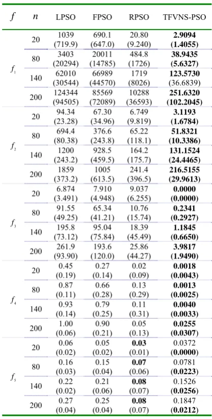
To illustrate the effectiveness and robustness of TFVNS-PSO algorithm for optimization problems, a set of 5 representative benchmark functions was employed to evaluate it in comparison with LPSO, FPSO, and RPSO [7].
The same initialization range [ 5,5]− and the constants
min min
V = X = -10 and V =Xmax max = 10 were used. At each algorithm, the number of particles was 20. The max iterations of these algorithms were all 300. A total of 30 repeated for each experimental setting were conducted and the averages as well as the standard deviations of these optimization results are computed.
The table I lists the testing results on the functions of
1
f ,f2,f3 ,f4 andf5.
TABLE I.
THE AVERAGES OF THE OPTIMIZATION RESULTS FOR THE FIVE BENCHMARK FUNCTIONS AND THEIR CORRESPONDING STANDARD
DEVIATIONS IN THE PARENTHESES.
f n LPSO FPSO RPSO TFVNS-PSO
1 f
20 (719.9) 1039 (647.0) 690.1 (9.240) 20.80 2.9094
(1.4055)
80 (20294) 3403 (14785) 20011 (1726) 484.8 38.9435
(5.6327)
140 (30544) 62010 (44570) 66989 (8026) 1719 (36.6839) 123.5730
200 (94505) 124344 (72089) 85569 (36593) 10288 251.6320
(102.2045)
2 f
20 (23.28) 94.34 (34.96) 67.30 (9.819) 6.749 3.1193
(1.6784)
80 (80.38) 694.4 (243.8) 376.6 (118.1) 65.22 51.8321
(10.3386)
140 (243.2) 1200 (459.5) 928.5 (175.7) 164.2 131.1524
(24.4465)
200 (373.2) 1859 (613.5) 1005 (396.5) 241.4 216.5155
(29.9613)
3 f
20 (3.491) 6.874 (4.948) 7.910 (6.255) 9.037 0.0000
(0.0000)
80 (49.25) 91.55 (41.21) 65.34 (15.74) 10.76 0.2341
(0.2927)
140 (73.12) 195.8 (75.84) 95.04 (45.49) 18.39 1.1845
(0.6650)
200 (93.90) 261.9 (120.0) 193.6 (44.27) 25.86 3.9817
(1.9490)
4 f
20 (0.19) 0.45 (0.14) 0.27 (0.09) 0.02 0.0018
(0.0043)
80 (0.11) 0.87 (0.28) 0.66 (0.29) 0.13 0.0013
(0.0025)
140 (0.14) 0.93 (0.25) 0.79 (0.31) 0.11 0.0040
(0.0033)
200 (0.06) 1.00 (0.21) 0.90 (0.13) 0.05 0.0255
(0.0307)
5 f
20 (0.02) 0.06 (0.02) 0.05 (0.01)0.03 (0.0372
0.0000)
80 (0.03) 0.16 (0.04) 0.15 (0.06) 0.07 (0.0781
0.0223)
140 (0.02) 0.22 (0.06) 0.21 (0.07) 0.08 (0.1526
0.0256)
200 (0.04) 0.27 (0.04) 0.25 (0.07)0.08 (0.1847
0.0212)
Benchmark functions
1 2 2 2
1 1 1
min ( ) n (100( ) ( 1) )
i i i
i
f x − x+ x x
=
=
∑
− + − ,10 xi 10,i {1, 2,..., }n
2
2 1
min ( ) n ( 10cos(2 ) 10)
i i
i
f x =
∑
= x − πx + ,10 xi 10,i {1, 2,..., }n
− ≤ ≤ ∈ .
2
3 1
min ( ) n i i
f x x
=
=
∑
,− ≤ ≤10 xi 10, i∈{1,2,..., }n .2 1
4 4000 1 1
min ( ) cos( ) 1i
n
n x
i i
i i
f x = x
=
=
∑
+ ∏ + ,10 xi 10,i {1, 2,..., }n
− ≤ ≤ ∈ .
2 2 1
2 2 1
(sin ) 0.5
5 (1 0.001 )
min ( ) 0.5
n i i
n i i
x
x
f x =
=
−
+
∑
= + ∑ ,
10 xi 10,i {1,2,..., }n
− ≤ ≤ ∈ .
From table I, the TFVNS-PSO is obviously excellent in both convergence and robustness for f1, f2, f3 and f4.
For f5, the TFVNS-PSO shows little efficiency, but it
improves the robustness considerably.
B. Discussion
The TFIWAC denotes without employing HNSOP, HNSTP and HNSGBP, namely, only improved PSO based on the TFIW and TFAC. A modified TFIWAC using HNSOP is denoted by HNSOP. And a modified TFIWAC using HNSTP is denoted by HNSTP. And a modified TFIWAC using HNSGBP is denoted by HNSGBP.
Further, to demonstrate the efficiency of TFIWAC, HNSOP, HNSTP and HNSGBP, the benchmark function
6
f was employed. Many authors tested algorithm using it
widely.
Benchmark function 100
4 2
1
6 100
1
min ( ) ( i 16 i 5 )i
i
f x x x x
=
=
∑
− + ,10 xi 10,i {1,2,...,100}
− ≤ ≤ ∈ .
The function f6 has about 2100 the local optimums in
the feasible solution space, and the global optimum is−78.3323.
With respect to the expected number of required function evaluations, the terminate criteria is
min 3
6 6 10
f − f∗ < − (f6∗= −78.3323). The PSO parameters
are set to their default values, ω=0.729 , c1=2.0 ,
2 1.8
c = . The TFIWAC, HNSOP, HNSTP and HNSGBP
parameters are setb=2, α =0.25, β =0.25, γ =0.25 and T=6000. The swarm size is 100 and the maximum generation is 6000 in five algorithms. Each group test includes 30 independent experiments. The experimental results are shown in the figure 4 and figure 5.
Figure 4. The average value.
Figure 5. The standard deviation.
0 1 2 3 4 5 6
PSO TFIWAC HNSOP HNSTP HNSGBP
S
ta
nd
ar
d
D
ev
ia
tio
n
-90 -80 -70 -60 -50 -40 -30 -20 -10 0
PSO TFIWAC HNSOP HNSTP HNSGBP
A
ve
rag
e
V
alu
Obviously, the several conclusions can be got from the figure 4 and figure 5. Firstly, the TFIWAC is superior to PSO in the efficiency (the smaller average, the better efficiency; and the smaller standard deviation, the better robustness.). Secondly, the HNSTP is the most excellent in both convergence and robustness. Finally, the HNSOP and the HNSGBP improve the efficiency of the TFIWAC little, but they enhance the robustness of the TFIWAC remarkably.
V. CONCLUSIONS
A novel improved PSO algorithm is proposed in this paper. Our main contribution is the modification of the parameters update rule and the heuristic variable neighborhood search strategies of particle swarm optimization. On the one hand, dynamic inertia weight based on the trigonometric functions of iterations is discussed, and then the dynamic acceleration coefficients based on the trigonometric functions of iterations is considered under the inertia weight of trigonometric function. On the other hand, through analyzing the behavior of the PSO, three novel heuristic variable neighborhood search rules are suggested to enhance the robustness and convergence. Compared with PSO and the other algorithms, the TFVNS-PSO demonstrates its superiority in convergence, robustness and solution quality, because the TFVNS-PSO has powerful global exploration at the beginning and ending of the evolution, and strongly local exploitation in the interim of run.
In the future, the sensitivity of TFVNS-PSO parameters: b,α, β, γ and Tshould be discussed. The
proposed approach should be used to solve other discrete combinatorial optimization problems such as flow shop scheduling problem and job shop scheduling problem.
ACKNOWLEDGMENT
The authors would like to thank anonymous reviewers and the editors for constructive comments and suggestions. This work is supported by the Special Talent Foundation of Ningxia Medical University in 2011.
REFERENCES
[1] J. Kennedy, R. Eberhart, “Particle Swarm optimization,”
IEEE Int. Conf. on Neural Networks, Perth, WA, Australia,
vol.4, pp. 1942–1948, Nov/Dec.1995.
[2] J. Kennedy, R.C. Eberhart, “A new optimizer using particle swarm theory,” Sixth Int. Symp. on Micro Machine and Human Science, Nagoya, Japan, pp. 39–43, Oct. 1995.
[3] C. J. Lin, M. H. Hsieh, “Classification of mental task from EEG data using neural networks based on particle swarm optimization,” Neurocomputing, vol.72 Issue 4/6, pp.
1121-1130, January 2009.
[4] G. Moslehi, M. Mahnam, “A Pareto approach to multi-objective flexible job-shop scheduling problem using particle swarm optimization and local search,”
International Journal of Production Economics, Vol. 129,
Issue 1, pp. 14-22, January 2011.
[5] C. Karakuzu, “Retraction notice to: Fuzzy controller training using particle swarm optimization for nonlinear
system control,” ISA Transactions, Vol. 48, Issue 2, pp. 245, April 2009.
[6] P. Chakraborty, S. Das, G. G. Roy, et al., “On convergence of the multi-objective particle swarm optimizers,”
Information Sciences, Vol. 181, Issue 8, pp. 1411-1425,
April 2011.
[7] Q. Luo, D.Y. Yi, “A co-evolving framework for robust particle swarm optimization,” Applied Mathematics and Computation, Vol. 199, Issue 2, pp. 611–622, June 2008.
[8] X.M. Yang, J.S. Yuan, J.Y Yuan, H.N. Mao, “A modified particle swarm optimizer with dynamic adaptation.”
Applied Mathematics and Computation, Vol. 189, Issue 2,
pp. 1205–1213, June 2007.
[9] S.F. Fan, E. Zahara, “A hybrid simplex search and particle swarm optimization for unconstrained optimization,”
European Journal of Operational Research, Vol. 181, Issue 2, pp. 527–548, September 2007.
[10] Y. Jiang, T.S. Hu, C.C. Huang, X.N. Wu, “An improved particle swarm optimization algorithm,” Applied Mathematics and Computation, Vol.193, Issue 1, pp. 231– 239, October 2007.
[11] F. van den Bergh, A.P. Engelbrecht, “A study of particle swarm optimization particle trajectories,” Information Sciences, Vol. 176, Issue 1, pp. 937–971, April 2006. [12]M. Jiang, Y.P. Luo, S.Y. Yang, “Stochastic convergence
analysis and parameter selection of the standard particle swarm optimization algorithm,” Information Processing Letters, Vol.102, Issue 1, pp. 8–16, April 2007.
[13]B. Jiao, Z.G. Lian, X.S. Gu, “A dynamic inertia weight particle swarm optimization algorithm,” Chaos, Solitons and Fractals, Vol.37, Issue 3, pp. 698–705, August 2008.
[14]A. S. Mohais, C. Ward, C. Posthoff, “Randomized directed neighborhoods with edge migration in particle swarm optimization,” Proceedings of the IEEE Congress on Evolutionary Computation, Vol.1, pp.548–555, June 2004.
[15]S. Janson, M. Middendorf, “A hierarchical particle swarm optimizer and its adaptive variant,” IEEE Trans. on Syst., Man, and Cybern., Part B: Cybern., Vol. 35, Issue 6, pp. 1272–1282, Dec. 2005.
[16]Y. Liu, Z. Qin, Z.W. Shi, J. Lu, “Center particle swarm optimization,” Neurocomputing, Vol. 70, Issue 4/6, pp.
672–679, January 2007.
[17]X.H. Shi, Y.C. Liang, H.P. Lee, et al., “An improved GA
and a novel PSO-GA-based hybrid algorithm,” Information Processing Letters, Vol. 93, Issue 5, pp. 255–261, March
2005.
[18]M. Senthil Arumugam, M.V.C. Rao, “On the improved performances of the particle swarm optimization algorithms with adaptive parameters, cross-over operators and root mean square (RMS) variants for computing optimal control of a class of hybrid systems,” Applied Soft Computing, Vol. 8, Issue 1, pp. 324–336, January 2008.
[19]Y.H. Shi, R. Eberhart, “A modified particle swarm optimizer,” IEEE Congress on Evolutionary Computation,
pp. 69–73, May 1998.
[20]A. Ratnaweera, S.K. Halgamuge, H.C. Watson. “Self-organizing hierarchical particle swarm optimizer with time-varying acceleration coefficients,” IEEE transactions on evolutionary computation, Vol.8, Issue 3, pp. 240–255, June 2004.
[21]P.V. Hentenryck, L. Michel, Constraint-based local search, the MIT Press, Cambridge, 2009.
Research, Vol. 37, Issue 11, pp. 1952-1964, November
2010.
[23]E. K. Burke, J.P. Li, R. Qu, “A hybrid model of integer programming and variable neighborhood search for highly-constrained nurse rostering problems,” European Journal of Operational Research, Vol. 203, Issue 2, pp. 484-493,
June 2010.
[24]S. Mitrović-Minić, A. P. Punnen, “Local search intensified: Very large-scale variable neighborhood search for the multi-resource generalized assignment problem,” Discrete Optimization, Vol. 6, Issue 4, pp. 370-377, November
2009.
[25]A. Bagheri, M. Zandieh, “Bi-criteria flexible job-shop scheduling with sequence-dependent setup times— Variable neighborhood search approach,” Journal of Manufacturing Systems, Vol. 30, Issue 1, pp. 8-15, January 2011.