Iterative Learning Control on Carrying Robot
Xiuxia Yang Yi Zhang Jianhong Shi
Department of Control Engineering, Naval Aeronautical and Astronautical University, Yantai, China Email: [email protected]
Xiaowei Liu
Graduate fourth team, Naval Aeronautical and Astronautical University, Yantai, China
Abstract—At present, most of the control methods of the lower extremity exoskeleton carrying robot require to calculate the system’s dynamic equation and create the control quantity at each moment, which don’t make full use of the repeatability feature of human movement and inevitably causes the delay on the dynamic response of the system. In this paper, utilizing the dynamic repeat characteristics of human walking, the time-variable quasi-Newton iterative learning controller of the lower extremity exoskeleton carrying system is designed to improve the control speed and the precision, where the human-machine interaction is considered . When the modeling error is large or the dynamics equation is not so accurate, the feedback loop can be added to improve the system’s performance. In this paper, the corresponding quasi-Newton method based on feedback is constructed, which is used to control the carrying robot. Simulation results show the valid of the given method.
Index Terms—Iterative learning control; Quasi-Newton method; Feedback; Carrying robot
I. INTRODUCTION
Lower extremity exoskeleton carrying system is a typical human-machine intelligent robot system, which combines the human intelligence and the machine mechanical energy. For the exoskeleton system unique human-machine control, it has become a new control problem that provokes widely interests of international learners[1].
The first prototype of exoskeleton named hardiman build by General Electric appears in 1968 [2]. Hardiman is set on master-slave control. In the case of a robotic arm the motion of the operator's arm must be captured continuously through the use of an instrumented master exoskeleton worn by the user. For the many and uncertain interface points between the human and the exoskeleton, the control method is unreliable. In robotic force control systems the force between the manipulator and its environment is maintained at a predetermined level through force sensor feedback. Eppinger[3], Whitney[4], and Craig[5]have described the traditional applications of
force feedback in robot manipulator control. In force feedback control all interaction forces are measured and there is no other contact point between the human and the machine than through the force sensor. Although it is theoretically possible to build such a control law it would be quite difficult to implement the hardware associated with it. The mostly successful exoskeleton HAL (Hybrid Assistive Leg)[6,7] use the s-EMG (surface ElectroMyogram) to sense the neuromuscular signal which are generated when motion, but there are many disadvantages when using s-EMG, for example, surface electrode is prone to fall off and the accuracy of the electrode will be influenced when people perspiring after a long time locomotion. The latest research results in this area come out of the BLEEX (Berkeley Lower Extremity Exoskeleton) [8], [9], [10]. Racine proposed a method named virtual joint torque control [11,12], and apply it into the BLEEX. The virtual joint torque control needs no direct measurements from the pilot or the human-machine interface (e.g. no force sensors between the two); instead, the controller estimates, based on measurements from the exoskeleton suits only, how to move so the pilot feels very little force. This control scheme is an effective method of generating locomotion when the contact location between the pilot and the exoskeleton is unknown and unpredictable. The main disadvantage of this control law over master-slave and feedback force control is that of the exoskeleton accurate mass properties must be known, otherwise, the error will be large.
The above control methods require to calculate the system’s dynamic equation and the control algorithm at each moment, which don’t make full use of the repeatability feature of human movement , which will inevitably causes the unnecessary waste of the resources, and there will be corresponding delay on the dynamic response of the system . After walking for a period of time in normal, according to the biomechanical model of human walking and some information of the wearer, add the learn control to the exoskeleton, and the energy consumption of the human and the exoskeleton can be reduced.
Model predictive[13], neural network study, iterative learning control can be used to the learning control, where iterative learning control is propitious to control the lower extremity exoskeleton system with dynamic repeat characteristics, which can implement the trace mission completely over the finite time interval and
1
q
2
q
3
q
t
L
Gt
L
s
L
Gs
L
Gf
L Hip
Knee
Ankle Thigh
Shank
Foot
Gt
Gs
Gf
Gf
h
Gs
h
Gt
h
Figure 1. Three segment model of the carrying robot leg
improve the tracking velocity and accuracy. In accordance with the difference of individuals, judge the wearers’ gait characteristics according to the human walking gait feature. Combing with the biomechanical modal, add learning control to the lower extremity exoskeleton.
For the carrying robot is a time-variable system with repeat characteristics, while the learning-factors in the general PID-style iterative learning control are constants which is fixed in advance and can not be changed with the system, good iterative convergent velocity can not be gotten. Therefore, choosing an appropriate time-variable learning operator and constructing the corresponding iterative learning control law become very important. Different to general robot system, for the interference of human in the carrying system, the human-machine interaction should be considered. Reference to the iteration study control of robot[14], the quasi-Newton method of the carrying robot is presented. When the model error is large or the dynamics equation is not accurate, the feedback loop can be added to improve the system’s performance. In this paper, the corresponding quasi-Newton method based on feedback is constructed, which is used to control the carrying robot.
II. CARRYING ROBOT DYNAMICS MATHEMATICS MODEL
Carrying robot is a new concept human-machine
intelligent robot system. The exoskeleton robot should shadow the motions of the human and never interfere with these motions. Figure 1gives a simplified three segment model of the carrying robot leg.
The swing phase of the carrying robot leg is taken as control object In this model, the inertia frame is chosen as the upper body and the exoskeleton leg in swing is assumed to be an independent 3-segment manipulator (thigh, shank and foot) pinned to the upper body at the hip. The length of the thigh link is
L
t, and the length of the shank link isL
s.The position of the centre of the gravity of the thigh byL
Gtandh
Gt, that of the shank byGs
L
andh
Gs, and that of the foot byL
Gf andh
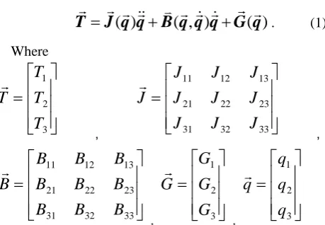
Gf asshown. The dynamic model can be written in a general form:
(1)
( )
( , )
( )
T
=
J q q
+
B q q q G q
+
. (1) Where⎥
⎥
⎥
⎦
⎤
⎢
⎢
⎢
⎣
⎡
=
3 2 1
T
T
T
T
,
⎥
⎥
⎥
⎦
⎤
⎢
⎢
⎢
⎣
⎡
=
33 32 31
23 22 21
13 12 11
J
J
J
J
J
J
J
J
J
J
,
⎥
⎥
⎥
⎦
⎤
⎢
⎢
⎢
⎣
⎡
=
33 32 31
23 22 21
13 12 11
B
B
B
B
B
B
B
B
B
B
,
⎥
⎥
⎥
⎦
⎤
⎢
⎢
⎢
⎣
⎡
=
3 2 1
G
G
G
G
,
⎥
⎥
⎥
⎦
⎤
⎢
⎢
⎢
⎣
⎡
=
3 2 1
q
q
q
q
J
is the inertia matrix and is a function ofq
,B
isthe centripetal and Coriolis matrix and is a function of
q
and
q
,G
is a vector of gravitational torques and is afunction of
q
only.Assume the total torque exerted on the joint is:
T
=
T
hm+
T
aThe damping and kinetic friction torque, stiffness torque and static friction torque are not considered in this sample because they can be impaired by subtract them in the controller.
In equation(1),
hm a
T
=
T
+
T
,T
hm denote the torqueexerted on the plant by human.
a
T
denote the torque exerted by actuator.The spring-damper device can be used to simulate
hm
T
:hm
T
=(
)
(
)
f d
k
q
q
k q
q
h
− +
h
−
Let
u t
( )
=a
T
, then( )
( , )
( )
(
)
(
)
=
+
+
−
−
−
−
f
d
u
J q q
B q q
G q
k
q
q
h
k q
q
h
. (2)
III.TIME-VARYING ITERATIVE LEARNING CONTROL OF
CARRYING ROBOT
A. Quasi-Newton Learning Method
Let the system be described by the operator
:
F U
→
Y
,whereU Y
,
are Banach spaces. Moreover suppose that the system works cyclically, that is during each cycle we have( )
(
( )),
0,1,
k k
y t
=
f u t
k
=
.Where
,
k k
y
∈
Y u
∈
U
are the control and the observable output of the system at k-th cycle, respectively. And we provide during each cycle the system are running between the finite time interval [0,T
]. Letdesired behavior of the system .Our aim is to find the control
d
u
which is a solution of the operator equation( )
(
( ))
d d
y t
=
f u t
.
Let us consider the iterative learning control scheme
1
( )
( )
(
( )) ( ),
0,1,
,
[0, ]
k k k k
u
+t
=
u t
−
L u t e t k
=
t
∈
T
(3)
where
e t
k( )
=
y t
k( )
−
y t
d( )
is the error at the k-thcycle and
L u t
(
k( ))
is a linear operator . If1
(
k( ))
[ '(
k( ))]
L u t
=
F u t
− ,where'(
k( ))
k
F
F u t
u
∂
=
∂
,then the learning control scheme becomes the classical Newton method. However, the operator F is often not given precisely . Therefore it is possible to take only some approximation of
F u t
'(
k( ))
as the learning operator .In paper[15], the theorem about the quasi-Newton method convergence is given:Theorem 1: Let
F U
:
→
Y
be continuouslydifferentiable in
(
d, )
{
d}
S u r
=
u
∈
U u
−
u
<
r
where r>0.Let the operator
L u
( )
be well defined inS u r
(
d, )
and suppose that the following conditions hold.
1)
L u
( )
≤
β
,
u
∈
S u r
(
d, )
2)
F u
'( )
1−
F u
'( )
2≤
γ
u
1−
u
2, ,
u u
1 2∈
S u r
(
d, )
3)
L u F u
( ) '( )
− ≤ <
I
δ
1,
u
∈
S u r
(
d, )
Then there exists
ε
>
0
such that for all0
(
d, )
u
∈
S u r
, the iterative learning control is convergent. The rate of convergence is linear and can be estimated by1
2
α δ
= +
βγε
B. Quasi-Newton Iterative Learning Control of the Lower Extremity Exoskeleton
The mission of control is to trace the anticipant repeated-running track
q t
d( )
,the carrying robot will be reset to the same beginning positionq
d(0)
after every work cycle completed. At the k-th work cycle, the controller outputs controlling torqueu t t
k( ),
∈
[0, ]
T
. Observe the output of the system( )
=
( )
k k
y t
q t
,
t
∈
[0, ]
T
and the error( )
=
( )
−
( )
k k d
e t
q t
q t
,
t
∈
[0, ]
T
,k
=
1, 2,
.Suppose the input signal is
u t
( )
andu t
( )
=T
a, we get( )
( , )
( )
(
)
(
)
=
+
+
−
f− −
d−
u
J q q
B q q
G q
k
q
q
k q
q
h
h
. (4)
Equation (4) satisfies Lipschitz qualification.
Linearize the track around the k-th work cycle of the equation of carrying robot:
(
)
(
,
)
(
(
,
)
(
)
(
)
)
∂
∂
∂
Δ +
Δ +
+
∂
∂
∂
∂
+
Δ − Δ − Δ = Δ
∂
k k k k k k
k k f d
B
B
G
J q
q
q q
q
q q
q
q
q
q
J
q q
q
k
q
k
q
u
q
(0)
0,
(0)
0
Δ
q
= Δ
q
=
. (5)Be noticed that the solution of the linear time-variable system mentioned above can be presented as
'(
( ))
Δ =
q
F u t
kΔ
u
, for( )
( )
( )
( )
Δ
q t
=
q t
d−
q t
k= −
e t
k ,design the learning scheme according to the equation(5):1
ˆ
ˆ
ˆ( )
(
,
)
(
(
,
)
ˆ
ˆ
(
)
(
)
)
ˆ
ˆ( )
(
(
,
)
)
ˆ
ˆ
ˆ
(
(
,
)
(
)
(
)
)
+
∂
∂
=
−
−
−
∂
∂
∂
∂
+
+
+
+
∂
∂
∂
=
−
−
−
∂
∂
∂
∂
−
+
+
−
∂
∂
∂
k k k k k k k k k
k k k k f k d k
k k k k k d k
k k k k k f k
B
B
u
u
J q e
q q e
q q
q
q
G
J
q
q q e
k e
k e
q
q
B
u
J q e
q q
k e
q
B
G
J
q q
q
q q
k e
q
q
q
(6) Where
k
=
1, 2,
,the initial value can be chosen as:0
=
( )
=
ˆ
(
d( ))
d( )
+
ˆ
(
d( ),
d( ))
+
ˆ
(
d( ))
u
u t
J q t q t
B q t q t
G q t
ˆ
ˆ ˆ
, ,
J B G
are the estimated values ofJ B G
, ,
.The learning law above is the application of the equation (3) on the lower extreme exoskeleton, and if
2
2
ˆ
ˆ
(
))[ ]
(
)
[ ] (
(
,
)
)
[ ]
ˆ
ˆ
ˆ
(
(
,
)
(
)
(
)
)[ ]
∂
=
+
−
∂
∂
∂
∂
+
+
+
−
∂
∂
∂
i
i
i
i
k k k k k d
k k k k k f
d
B
d
q u
J q
q q
k
dt
q
dt
B
G
J
q q
q
q q
k
q
q
q
the control law is the same to formula (3) .
In order to give the convergence theorem of the lower extreme exoskeleton iterative learning , first to definite the system operator as
F
,andU Y
,
in Banach spaces. If the input of the system isu t t
( ),
∈
[0, ]
T
, according toF
, we can calculate the solutionq t
( )
of the dynamics2 [0, ]
sup
( )
C T
u
u t
2 2 2 2
[0, ] [0, ] [0, ]
sup
( )
sup
( )
sup
( )
C
T T T
q
q t
+
q t
+
q t
Where
•
2 is the Euclidean norm of the vector.Supposing
F
is continuously differentiable in the interval of ss, wherer
>
0
.Reference to paper [14, 15], on the following, the convergence theorem of the exoskeleton iterative learning is given.
Theorem 2: Suppose
F u
:
∈
C
[0, ]
T
→ ∈
q
C
2[0, ]
T
is theoperator associated with the lower extreme exoskeleton dynamics equation.
F
is continuously differentiable inthe interval of
S u r
(
d, )
= ∈
{
u U u u
−
d C<
r
}
, wherer
>
0
,u t
d( )
is the expected control input which is corresponding to the expected outputq t
d( )
,[0, ]
∈
t
T
. The following conditions are supposed to be true,1)
[0, ]
ˆ
ˆ( ( )) , ( ( ), ( )) ,
sup
ˆ
ˆ ˆ
( ( ), ( )) ( ( ), ( )) ( )
, ( )
B
J q q q K
q
B G J
q q q q q q K
q q q
q
β
∈
⎧ ∂ ⎫
−
⎪ ∂ ⎪
⎪ ⎪
⎨ ⎬
∂ ∂ ∂
⎪ + + − ⎪
⎪ ∂ ∂ ∂ ⎪
⎩ ⎭
≤ ∈ Δ
d
t T
k k f
t t t
t t t t
t
2)
u u
1,
2is the control input (controller output), and the corresponding system output isq
1=
F u
( )
1∈ Δ
and
q
2=
F u
(
2)
∈ Δ
. For anyv U
∈
, the solutionX X
1,
2 of the linear time-varying systems1 1 1 1 1 1 1
1 1 1 1
( )
(
( ,
)
)
(
( ,
)
( )
( )
)
B
B
J q x
q q
K
x
q q
q
q
G
J
q
q q
K
x
v
q
q
∂
∂
−
−
−
∂
∂
∂
∂
+
+
−
=
∂
∂
d
f
1
(0)
0, (0)
10,
x
=
x
=
and
2 2 2 2 2 2 2
2 2 2 2
(
)
(
(
,
)
)
(
(
,
)
(
)
(
)
)
B
B
J q x
q q
K
x
q q
q
q
G
J
q
q q
K
x
v
q
q
∂
∂
−
−
−
∂
∂
∂
∂
+
+
−
=
∂
∂
d
f
2
(0)
0,
2(0)
0,
x
=
x
=
satisfy the inequality
2
1 2 C 1 2 C C
x
−
x
≤
γ
u
−
u
v
3) For any
u
∈
S
(
u r
d, )
andv
∈
U
,x
is the solution of the following system:( ( ))
(
( ( ), ( ))
)
(
( ( ), ( ))
( ( ))
( ( )) ( )
)
B
J q u x
q u q u
K
x
B
G
q u q u
q u
q
q
J
q u q u
K
x
v
q
∂
−
−
∂
∂
∂
−
+
∂
∂
∂
+
−
=
∂
d
f
q
(0)
=
0, (0)
=
0,
x
x
There is a constant
δ
<
1
, which makes[0, ]
2
ˆ
ˆ
sup
( ( ))
( ( ), ( )
) ( )
ˆ
ˆ
(
( ( ), ( ))
( ( ))
ˆ
( ( )) ( )
) ( )
( )
B
J q u x
q u q u
K
x
q
B
G
q u q u
q u
q
q
J
q u q u
K
x
v
q
v
δ
∈
∂
+
−
∂
∂
∂
+
+
∂
∂
∂
+
−
−
∂
≤
d t T
f
C
t
t
t
Then there exists
ε
>
0
, which makes the iterative learning process ofu
0∈
S u
(
d, )
ε
convergent with the control law (6). The convergence rate can be estimated bythe following formula:
1
2
α δ
= +
βγε
Found by the derivation, there are not suitable points at the proofs of the literatures [14, 15], and is about the operating system for the robot. Combining with the exoskeleton system, the following gives the convergence proof of the quasi Newton iterative learning law.
Learning iterative control scheme of carrying robot with feedbacks is as follows:
1
1 1
ˆ
ˆ( )
(
(
,
)
)
ˆ
ˆ
ˆ
(
(
,
)
(
)
(
)
)
+
+ +
∂
=
−
−
−
−
∂
∂
+
∂
+
∂
−
∂
∂
∂
−
−
k k k k k k d k
k k k k k f k
v k p k
B
u
u
J q e
q q
k e
q
B
G
J
q q
q
q q
k e
q
q
q
K e
K e
(10)
Then equation above can be presented as:
1 , 1 , 1
k ff k fb k
u
+=
u
++
u
+Where,
, 1
ˆ
ˆ( )
(
(
,
)
)
ˆ
ˆ
ˆ
(
(
,
)
(
)
(
)
)
+
∂
=
−
−
−
∂
∂
∂
∂
−
+
+
−
∂
∂
∂
ff k k k k k k d k
k k k k k f k
B
u
u
J q e
q q
k e
q
B
G
J
q q
q
q q
k e
q
q
q
, 1 1 1
fb k v k p k
u
+= −
K e
+−
K e
+0
0 0
ˆ
ˆ
( )
(
( ))
( )
(
( ),
( ))
ˆ ( ( ))
=
=
+
+
−
−
d d d d
d v p
u
u t
J q t q t
B q t q t
G q t
K e
K e
When
K
v,K
pare assigned reasonable values.Also, control scheme(9) can be overwritten as
1
1 1
ˆ
ˆ( ) ( ( , ) )
ˆ
ˆ ˆ
( ( , ) ( ) ( ) )
+
+ +
∂
= − − − −
∂
∂ +∂ +∂ −
∂ ∂ ∂
− −
k k d k d d d k
d d d d d f k
v k p k
B
u u J q e q q k e
q
B G J
q q q q q k e
q q q
K e K e
(11)
Initial value is:
0
0 0
ˆ
ˆ
( )
(
( ))
( )
(
( ),
( ))
( )
ˆ ( ( ))
=
=
+
+
−
−
d d d d d
d v p
u
u t
J q t q t
B q t q t q t
G q t
K e
K e
(12)
IV.ITERATIVE LEARNING CONTROL REALIZATION
Simulate swing stage of the lower extreme exoskeleton. In order to simplify the calculation, assuming
0
=
=
=
Gf Gs Gt
h
h
h
in equation (1), that is, the centerof gravity of each segment is in the center line.
The learning gain is chosen
as
K
P=
diag
(10,10, 5)
,K
v=
diag
(1,1, 0.2)
. Themaximum iteration times
k
and the allowed tracking accuracyε
isk
=
50
,ε
=
0.02
.In the simulation examples, after 7 iterations, the outputs of the actual controlled system reach to the desired tracking accuracy, the convergence process of the respective joints are shown in Figures 2-4. After learning, the human-machine interference force and the torque applied by the actuator are shown in Figure 5.
As can be seen from the figures, although there is an error in Lagrange mathematical model, after learning, the angle output of the exoskeleton is able to track the wearer's angle output, the human-machine interference force is very small, and the exoskeleton carrying function can be realized.
0 0.05 0.1 0.15 0.2 0.25 0.3 0.35 0
0.1 0.2 0.3 0.4 0.5 0.6 0.7 0.8
time(s)
hip(
ra
d)
Figure2. Hip angle tracking curve
0 0.05 0.1 0.15 0.2 0.25 0.3 0.35
-1 -0.9 -0.8 -0.7 -0.6 -0.5 -0.4 -0.3 -0.2 -0.1
time(s)
k
n
e
e
(rad
)
Figure3. Knee angle tracking curve
0 0.05 0.1 0.15 0.2 0.25 0.3 0.35
-0.2 -0.15 -0.1 -0.05 0 0.05 0.1 0.15
time(s)
an
k
le
(r
a
d)
Figure4. Ankle angle tracking curve
0 0.05 0.1 0.15 0.2 0.25 0.3 0.35 0.4 0.45 0.5
-50 0 50
time(s)
h
ip t
o
rq
ue
(Nm
)
0 0.05 0.1 0.15 0.2 0.25 0.3 0.35 0.4 0.45 0.5
-20 0 20
time(s)
k
n
e
e
t
o
rq
u
e
(Nm
)
0 0.05 0.1 0.15 0.2 0.25 0.3 0.35 0.4 0.45 0.5
0 1 2
time(s)
an
k
le t
or
que(
N
m
)
actuator human
actuator human
actuator human
Figure5. Torque applied by the operator and the the drive
V.CONCLUSION
Using the repetition characteristics of the lower extreme carrying system, according to the theory of the quasi Newton iterative learning law, the time-varying operator of the lower extreme exoskeleton iterative learning is constructed.
the swing phase, the lower extremity exoskeleton iterative learning control is realized. The simulation results show the effectiveness of this method. The following work is to combine this method with the virtual torque control method to improve the speed and accuracy of the control.
REFERENCES
[1] T. Bock, T. Linner and W. Ikeda (2012). Exoskeleton and Humanoid Robotic Technology in Construction and Built Environment, The Future of Humanoid Robots - Research and Applications.
[2] http://www.davidszondy.com/future/robot/hardiman.htm [3] Eppinger S.D., Seering W.P.,"Understanding Bandwidth
Limitations in Robot Force Control", Proceeding of the IEEE International Conference on Robotics and Automation, 1987, pp904-909.
[4] Whitney D.E., "Historical Perspective and State of the Art in Robot Force Control", The International Journal of Robotics Research, Vol. 6, No. 1, Spring 1997.
[5] Craig J. J., "Introduction to Robotics", Addison-Wesley Publishing Co., 1998.
[6] Lee S. and Sankai Y. “Power assist control for walking aid with HAL-3 based on EMG and impedance adjustment around knee joint”, In Proc. Of IEEE/RSJ International Conf on Intelligent Robots and Systems (IROS 2002), EPFL, Switzerland, pp. 1499-1504, 2002
[7] Hiroaki Kawamoto and Yoshiyuki Sankai, “Power assist system HAL-3 for gait disorder person”, K. Miesenberger, J. Klaus, W. Zagler (Eds.): ICCHP 2002, LNCS 2398, pp. 196-203, 2002.
[8] Adam B. Zoss, H. Kazerooni, and Andrew Chu, “Biomechanical design of the berkeley lower extremity exoskeleton (BLEEX)”, IEEE/ASME Transactions on Mechatronics, Vol.11, No.2, April, 2006
[9] A. Chu, H. Kazerooni, and A. Zoss, “On the biomimetic design of the berkeley lower extremity exoskeleton (BLEEX)”, in Proc. IEEE ICRA, Barcelona, Spain, pp. 4345–4352, Apr. 18–22, 2005
[10]J. L. Racine, “Control of a lower extremity exoskeleton for human performance amplification,” Ph. D. dissertation, University of California, Berkeley, 2003.
[11]H. Kazerooni, L. Huang, and R. Steger, “On the control of the berkeley lower extremity exoskeleton (BLEEX)”, in IEEE ICRA, Barcelona, Spain, pp. 4353–4360, Apr. 18–22, 2005
[12]J. R. Steger, “A design and control methodology for human exoskeletons,” Ph. D. dissertation, University of California, Berkeley, 2006.
[13]Letian Wang, Edwin H. F. van Asseldonk, Herman van der Kooij. “Model Predictive Control-based Gait Pattern Generation for Wearable Exoskeletons”. 2011 IEEE International Conference on Rehabilitation Robotics, 2011
[14]Yao Yuan, “Robot iterative learning control algorithm application research”. Zhejiang University, 2004
[15]K. E. Avrachenkov, “Iterative learning control based on quasi-Newton methods” , in Proc.1998 Conf. Decision and Control, pp.170-174, 1998
[16]Kirtley C.,Hong Kong Polytechnic
University,Http://guardian.curtin.edu.au:16080/cga/data/H Kfyp98/All.gcd
Xiuxia Yang was born in Laizhou, Shandong Province, China in 1975. He received his Ph.D. degree in electrical engineering from naval university of engineering,Wuhan, China in 2005. Since 2000, he has been with department of control engineering of naval aeronautical and astronautical university, where he is currently a vice professor.
His main research interests include nonlinear control theory with applications to robots, aircraft and other mechanical systems.\
Yi Zhang was born in Rongcheng, Shandong Province, China in 1971. He received his master degree in control theory and application from naval aeronautical and astronautical university,Yantai, China in 2001. Since 2000, he has been with department of control engineering of naval aeronautical and astronautical university, where he is currently a vice professor.
His main research interests include nonlinear control theory with applications to robots, aircraft and other mechanical systems.
Jianhong Shi was born in Wujing, Jiangsu Province, China in 1963. He received his master degree in control theory and application from naval aeronautical and astronautical university,Yantai, China in 1989. Since 1989, he has been with department of control engineering of naval aeronautical and astronautical university, where he is currently a vice professor.
His main research interests include nonlinear control theory with applications to robots, aircraft and other mechanical systems.
XiaoweiLiu was born in Zaozhuang,Shandong Province, China in 1986. He received his bachelor degree in spacecraft engineering from naval aeronautical and astronautical university,Yantai, China in 2008. He is currently working toward the master degree in control theory and application at naval aeronautical and astronautical university.