An Adaptive LMS Channel Estimation Method for LTE SC-FDMA Systems

An Adaptive LMS Channel Estimation Method for

LTE SC-FDMA Systems

Md. Masud Rana, Jinsang Kim, and Won-Kyung Cho

Department of Electronics and Radio Engineering Kyung Hee University

Yongin Gyeonggi, Republic of Korea Email: [email protected]

Abstract— 3rd generation partnership project (3GPP) long term evolution (LTE) uses single carrier-frequency division multiple access (SC-FDMA) in uplink transmission and orthogonal frequency division multiple access (OFDMA) scheme for the downlink. One of the most important challenges for a transceiver design is channel estimation (CE) and equalization. In this paper, a training based least mean square (LMS) CE method is investigated for a LTE SC-FDMA system. This method can avoid the ill-conditioned least square (LS) problem. In addition, this CE method uses adaptive estimator which is able to update parameters of the estimator continuously. Simulation results show that the LMS CE technique with 500 Hz Doppler frequency has around 3 dB better performances compared with 1.5k Hz Doppler frequency.

Index Term— Channel estimation, least square, LMS, SC-FDMA.

I. INTRODUCTION

The wireless evolution has been stimulated by an explosive growing demand for a wide variety of high quality of services in voice, video, and data. This rigorous demand has made an impact on current and future wireless applications, such as digital audio/video broadcasting, wireless local area networks (WLANs), worldwide interoperability for microwave access (WiMAX), wireless fidelity (WiFi), cognitive radio (CR), and 3rd generation partnership project (3GPP) long term evolution (LTE) [1], [2]. LTE uses uses single carrier-frequency division multiple access (SC-FDMA) in uplink transmission and orthogonal frequency division multiple access (OFDMA) scheme for the downlink [1]. A highly efficient way to cope with the frequency selectivity of wideband channel is OFDMA. OFDMA is an effective technique for combating multipath fading and for high bit rate transmission over mobile wireless channels. Channel estimation (CE) has been successfully used to improve the performance of the LTE OFDMA systems. It can be employed for the purpose of detecting received signal, improve signal-to-noise ratio (SNR), channel equalization, cochannel interference (CCI) rejection, and improved the system performance [3-5]. The training CE algorithm requires probe sequences; the receiver can use this probe sequence to reconstruct the transmitted waveform [6-8]. Training symbols can be placed either at the beginning of each burst as a preamble or regularly through the burst. Training sequences are transmitted at certain positions of the SC-FDMA frequency time pattern, in its place of data.

Several CE techniques have been proposed for LTE SC-FDMA systems. In [3], the least square (LS) CE has been proposed to minimize the squared differences between the received and estimated signal. The LS algorithm, which is independent of the channel model, is commonly used in equalization and filtering applications. But the statistics of channels in real world change over time. Another limitation that is encountered in the straight application of the LS estimator is that the inversion of the large dimensional square matrix turns out to be ill-conditioned. Two-dimensional based on Wiener filtering pilot symbol aided CE has been proposed [4]. Although it exhibits the best performance among the existing linear algorithms in literature, it requires accurate knowledge of second order channel statistics, which is not always feasible at a mobile receiver. This estimator gives almost the same result as 1D estimator, but it requires higher complexity. To further improve the accuracy of the estimator, Wiener filtering based iterative CE has been investigated [4], [7]. However, this scheme also requires high complexity and knowledge of channel correlations [9-12].

Adaptive CE has been, and still is, an area of active research topics, playing imperative roles in an ever growing number of applications such as wireless communications where the channel is rapidly time-varying. Signal processing techniques that use recursively estimated, time varying models are normally called adaptive. Different adaptive CE algorithms have been proposed over the years for the purpose of updating the channel coefficient. The least mean square (LMS) method, its normalized version (NLMS), the affine projection algorithm (APA), as well as the recursive least square (RLS) method are well known examples of such CE algorithms. The well known LMS/NLMS CE algorithms are attractive from a computational complexity point of view but their convergence behavior for highly correlated input signals is poor. The RLS CE method resolves this trouble, but at the expense of increased complexity. A very large number of fast RLS CE methods have been developed over the years, but regrettably, it seems that the better a fast RLS CE method is in terms of computational efficiency and numerical stability [13-15]. In addition, the RLS algorithm has the recursive inversion of an estimate of the autocorrelation matrix of the input signal as its cornerstone, problems arise, if the autocorrelation matrix is rank deficient.

are not required. This LMS CE algorithm requires knowledge of the received signal only. This can be done in a digital communication system by periodically transmitting a training sequence that is known to the receiver. Simulation results show that the LMS CE scheme with 500 Hz Doppler frequency has 3 dB better performances compared with 1.5 kHz Doppler frequency.

We use the following notations throughout this paper: bold

face lower letter is used to represent vector. Superscripts x* _and

xT _{denote the conjugate and conjugate transpose of the complex}

vector x respectively.

The remainder of the paper is organized as follows: section II describes LTE SC-FDMA systems model. The adaptive LMS CE method is presented in section III, and its performance is analyzed in section IV. Finally, conclusions are made in section V.

II. LTE SC-FDMA SYSTEMS MODEL

In this section, we briefly explain SC-FDMA system model, fading channel statistics, and received signal model.

A. Baseband system model

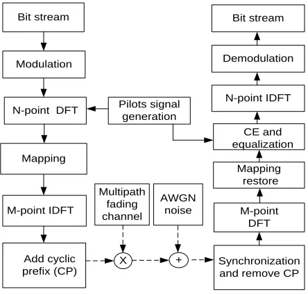
A baseband block diagram for the communications system under investigation is shown in Fig. 1.

CE and equalization Bit stream

Modulation

Add cyclic prefix (CP)

Synchronization and remove CP

M-point DFT N-point IDFT

X + Multipath

fading channel

AWGN noise N-point DFT

Mapping

Demodulation Bit stream

M-point IDFT

Mapping restore Pilots signal

generation

Fig. 1. Block diagram of a LTE SC-FDMA system.

At the transmitter, a baseband multiple phase shift keying modulator takes binary sequence and produces the signaling waveforms

i i

i i

i i

2E

m (t) =

cos(ωt + α ), 0 < t < T

T

2E

=

[cos(α ) cos(ωt) - sin(α ) sin(ωt)]

T

= a b(t) + c d(t), (1)

where T is the symbol duration, E is the energy of

m (t),

_i

ω = 2πf, f is the carrier frquency, phase anagle

2

i

, M

M







is the alphabate size,



_i



E

cos



_i inphase basis,

i i

2

b(t) =

cos(ωt), c =

sinα

T

E

, and quadrature basis,

2

d(t) = -

cos(ωt).

T

CE is often achieved by multiplexing

known symbols, so called, pilot symbols into data sequences [1]. These modulated symbols and pilots perform N-point discrete Fourier transform (DFT) to produce a frequency domain representation:

-j2 mt N-1

N

i i

t=0

1

s (t) =

m (t) e

, (2)

N





where j is the imaginary unit. It then maps each of the N-point DFT outputs to one of the orthogonal sub-carriers mapping that can be transmitted. There are two principal sub-carrier mapping modes: localized mode, and distribution mode. In distributed sub-carrier mode, the outputs are allocated equally spaced sub-sub-carrier, with zeros occupying the unused sub-carrier in between. While in localized sub-carrier mode, the outputs are confined to a continuous spectrum of sub-carrier. Interleaved sub-carrier mapping mode of FDMA (IFDMA) is another special sub-carrier mapping mode [16], [17]. The difference between DFDMA and IFDMA is that the outputs of IFDMA are allocated over the entire bandwidth, whereas the DFDMAs outputs are allocated every several subcarriers [18], [19].

Finally, the inverse DFT (IDFT) module output is followed by a cyclic prefix (CP) insertion that completes the digital stage of the signal flow. The CP is used to eliminate ISI and preserve the orthogonality of the tones. Assume that the channel length of CP is larger than the channel delay spread [20].

B. Channel model

Channel model is a mathematical representation of the transfer characteristics of the physical medium. These models are formulated by observing the characteristics of the received signal. According to the documents from 3GPP, a radio wave propagation can be described by multipaths which arise from reflection and scattering [20]. The received signal at the mobile terminal is a superposition of all paths. If there are L distinct paths from transmitter to the receiver, the impulse response of the multipath fading channel can be represented as [20]:

L

j j

j=1

ω(m,τ) =



ω (m)δ[m - τ (m)], (3)

where

ω (m)

_j and

τ (m)

_j are attenuations and delays for each

path at time instant m, and

δ(.)

is the Dirac delta function. The

j d

ω(v) = ω 1- (v/f ) , (4)

where Doppler frquency

f = s/λ,

_d s is the speed of the mobile,

and λ is the wavelength of the transmitted carrier. In order to do simulations as close to the reality as possible, it is essential to have a good channel model. This model is used to describe the fast variations of the received signal strength due to changes in phases when a mobile terminal moves. In case of wideband modeling, each path of the impulse response can be modeled as Rayleigh distributed with uniform phase except line of sight (LOS) component cases [20].

C. Received signal model

The transmitted symbols propagating through the radio channel can be modeled as a circular convolution between the

CIR and the transmitted data block i.e.,

[s(m)* (m, )]





. Since,

the channel coefficient is usually unknown to the receiver, it needs to be efficiently estimated. The impulse response of multipath fading channel can be represented by a tap-delayed line filter with time varying coefficients and symbol-rate spaced coefficients.

Delay _Delay

+ + +

Input

signal s(m-2) _{s(m-3) s(m-L)}

s(m-1) Delay

X _w2(m) X w3(m) X X

w1(m) wL(m)

Fig. 2. L-tapped delay line filter of a fading channel.

At the receiver, the opposite set of the operation is performed. After synchronization, CP samples are discarded and the remaining samples are processed by the DFT to retrieve the complex constellation symbols transmitted over the orthogonal sub-channels. The received signals are de-mapped and equalizer is used to compensate for the radio channel frequency selectivity. After IDFT operation, these received signals are demodulated and soft or hard values of the corresponding bits are passed to the decoder. The decoder analyzes the structure of received bit pattern and tries to reconstruct the original signal.

III. ADAPTIVE LMS CE METHOD

CE is the process of characterizing the effect of the physical medium on the input sequence. The aim of most CE algorithms is to minimize the mean square error (MSE), while utilizing as little computational resources as possible in the estimation process [2], [4]. CE algorithms permit the receiver to estimated the impulse response of the channel and clarify the behavior of the channel. This information of the channel’s behavior is well utilized in modern mobile radio communications. One of the most important benefits of CE is that it allows the

implementation of coherent demodulation. Coherent

demodulation requires the knowledge the phase of the signal.

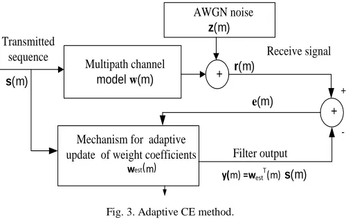
This can be accomplished by using CE techniques. Once a model has been established, its parameters need to be estimated in order to minimize the error as the channel changes. If the receiver has a priori knowledge of the information being sent over the channel, it can utilize this knowledge to obtain an accurate estimate of the impulse response of the channel. An adaptive algorithm is a process that changes its parameters as it gain more information of its possibly changing environment. Among numerous iterative techniques that exist in the open literature, the popular category of approaches which are obtain from the minimization of the MSE between the output of the filter and desired signal to perform CE as shown in Fig. 3.

-AWGN noise

z(m)

Receive signal

r(m) Transmitted

sequence

Multipath channel

model w(m) +

+

Mechanism for adaptive update of weight coefficients

west(m)

y(m)=westT(m)s(m)

+

s(m)

Filter output e(m)

Fig. 3. Adaptive CE method.

The signal s(m) is transmitted via a time-varying channel

w(m), and corrupted by an additive noise estimated by using any

kind of CE method. The main aim of most CE algorithms is to minimize the MSE i.e., between the received signal and its estimate. In the Fig 3, we have unknown multipath fading channel, that has to be estimated with an adaptive filter whose weight are updated based on some criterion so that coefficients of adaptive filter should be as close as possible to the unknown channel. The output from the channel can be expressed as:

L-1

l = 0

r(m) =



w(m,l) s(m - l) + z(m), (5)

where s(m - l) is the complex symbol drawn from a constellation

s of the lth paths at time m-l, L is the channel length, z(m) is the

additive white Gaussian noise (AWGN) with zero mean and

variance

σ

2. The above equation can be rewritten as vector

notation [1]:

(m) =

T

(m) (m) + (m), (6)

r

w

s

z

where

s

= (s , s ,...,s

_{0 1 L-1}

)

T,

r = (r , r ,...,r ) ,

_{0 1 L-1} T

T

0 1 L-1

= (w , w ,...,w

)

w

, and

z

= (z , z ,...,w

_{0 1 L-1}

) .

T

The output of the adaptive filter is

( )

m



T_est

( ) ( ), (7)

m

m

y

w

s

where

w

_est

( )

m

is the estimated channel coefficients at time m.

(m) = (m) - (m)

=

T

(m) (m) + (m)



T_est

( ) (m) (8)

m

e

r

y

w

s

z

w

s

This error signal is used by the CE to adaptively adjust the weight vector so that the MSE is minimized. Now the cost

function

j(m) = E[ (m) (m)]

e

e

* for the adaptive filter

structure is

* T T

est est

T

2 T T

est est

j(m) = E[

( ) ( )] - E[ ]

(m) - (m)

(m)

E[

]

( )

( ) [

( ) ( )]

=

( )

(m) -

(m)

( )

+ ( )

( )

( ), (

T

T T

est est

T r

T

est est

m

m

m

m E

m

m

m

m

m

m

m







r

r

s r w

r

w

s

w

w

s

s

c

w

w

c

D

w

w

9)

where



_r2 is the variance of the received signal,

( )

m



E[ (m) (m)]

T

c

s

r

is the cross-correlation vector

between the tap input vector s(m) and the received signal r(m),

and

D

(m) = E[ (m) (m)]

s

s

T is the correlation matrix of the

tap input vector s(m). Now taking the gradient vector with

respect to

w

_est

( )

m

:

T est

*

j(m) = -2 (m) + 2 (m)

(m)

= - 2 (m) ( ) + 2 (m) ( )

m

T

m

T_est

( ). (10)

m



c

D

w

s

r

s

s

w

According to the method of steepest descent, if

w

_est

(m)

is the

tap-weight vector at the mth iteration then the following

recursive equation may be used to update

w

_est

(m)

:

est est

* T

est est

* est

(m +1) =

(m) - 1/2 ηΔj(m)

=

(m) + η (m)[ (m) -

(m) (m)]

=

(m) + η (m) ( ), (11)

T

m

w

w

w

s

r

w

s

w

s

e

where

w

_est

(m+1)

denotes the weight vector to be computed at

iteration (m + 1) and

η

is the LMS step size which is related to

the rate of convergence. The smaller step size means that a longer reference or training sequence is needed, which would reduce the payload and hence, the bandwidth available for

transmitting data. The term [

η (m) (m)

s

e

* ] represents the

correction factor or adjustment that is applied to the current estimate of the tap-weight vector. The iterative procedure is

started with an initial guess

w

_est

(0)

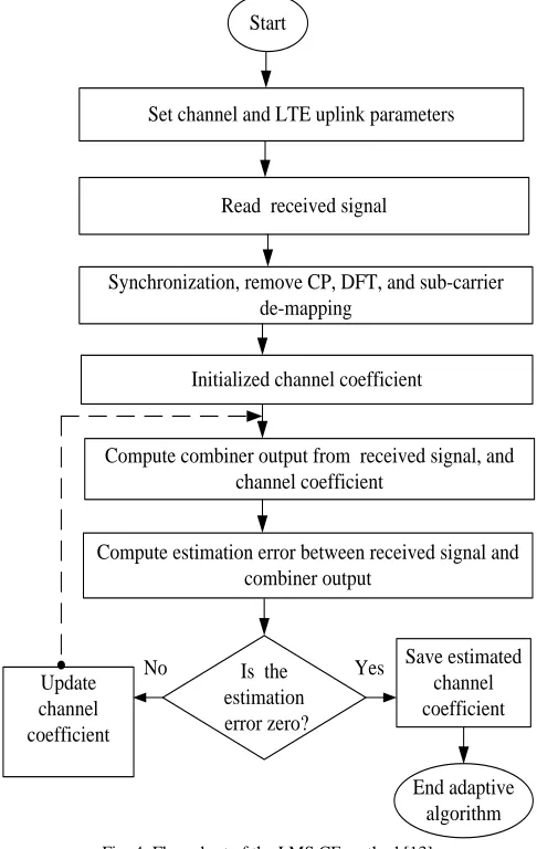
. The detail step of this CE

algorithm is shown in Fig. 4.

Start

Set channel and LTE uplink parameters

Read received signal

Update channel coefficient

No

End adaptive algorithm Yes

Is the estimation error zero?

Compute estimation error between received signal and combiner output

Save estimated channel coefficient Initialized channel coefficient

Compute combiner output from received signal, and channel coefficient

Synchronization, remove CP, DFT, and sub-carrier de-mapping

Fig. 4. Flow chart of the LMS CE method [13].

IV. PERFORMANCE ANALYSIS

A. Computational complexity

The complexity of CE is of crucial importance especially for time varying wireless communication channels, where it has to be performed periodically or even continuously. Table I summarizes the computational complexity of the LMS CE method, where L is the channel length, and real number indicates scalar operation.

TABLE I

COMPLEXITY PER ITERATION

Operation Complexity

Multiplication 7L + 1

Addition 9L - 3

B. Simulation results

SC-FDMA system in Doppler spread environments are summarized in Table II.

Table II

THE SYSTEMS PARAMETERS FOR SIMULATION

Systems parameters Assumptions

System bandwidth 5 MHz

Sampling frequency 7.68 MHz

Sub-carrier spacing 9.765 kHz

Modulation data type BPSK

FFT size 16

Sub-carrier mapping scheme IFDMA

IFFT size 512

Data block size 32

Cyclic prefix 4µs

Channel Rayleigh fading

LMS gain 0.4

Equalization ZF

Doppler frequency 100, and 1.5 kHz

Fig. 5 shows the MSE versus SNR for the LMS CE method with different Doppler frequencies. We can see that the LMS CE method with 500 Hz Doppler frequency has 3 dB better performances compared with 1500 Hz Doppler frequency. This CE method uses adaptive estimator which is able to update parameters of the estimator continuously, so that knowledge of

channel and noise statistics are not required.Such approach can

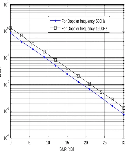
guarantee the convergence towards the true channel coefficient. The same behavior can be observed for BER performance in Fig. 6.

Fig. 5. MSE performance comparisons of the LMS CE method.

Fig. 6. BER performance comparisons of the LMS CE method.

V. CONCLUSION

In this paper, training based LMS CE scheme is investigate for a LTE SC-FDMA system that can avoid the ill-conditioned least square (LS) problem. This CE scheme uses adaptive estimator which is able to update parameters of the estimator continuously, so that knowledge of channel and noise statistics are not required. The computational complexities, MSE and BER performance, are analyzed and compared with the different Doppler frequencies. From computer simulations, we can come to the conclusion that the LMS CE method with 500 Hz Doppler frequency has 3 dB better performances compared with 1.5 kHz Doppler frequency.

ACKNOWLEDGMENT

This research was supported by the Basic Science Research Program through the National Research Foundation of Korea (NRF) funded by the Ministry of Education, Science and Technology (20100017118).

REFERENCES

[1] B. Karakaya, H.Arslan, and H. A. Cirpan, ”Channel estimation for LTE uplink in high Doppler spread,” Proc. Int. Con. on WCNC, pp. 1126-1130, April 2008.

[2] J. Berkmann, C. Carbonelli, F.Dietrich, C. Drewes, and W. Xu, ”On 3G LTE terminal implementation standard, algorithms, complexities and challenges,” Proc. Int. Con. on WCMC, pp. 970-975, August 2008.

[3] A. Ancora, C. Bona, and D.T.M. Slock,”Down-sampled impulse response least-squares channel estimation for LTE OFDMA,” Proc.

Int. Con. ASSP, vol. 3, pp. 293-296, April 2007.

[4] L. A. M. R. D. Temino, C. N. I Manchon, C. Rom, T. B. Sorensen, and P. Mogensen, ”Iterative channel estimation with robust wiener filtering in LTE downlink,” Proc. Int. Con. on VTC, pp. 1-5, September 2008.

0 5 10 15 20 25 30

10-4 10-3 10-2 10-1 100 101

SNR [dB]

M

S

E

For Doppler frequency 500Hz For Doppler frequency 1500Hz

0 5 10 15 20 25 30

10-4 10-3 10-2 10-1 100 101

SNR [dB]

BER

[5] S. Y. Park, Y.Gu. Kim, and C. Gu. Kang, ”Iterative receiver for joint detection and channel estimation in OFDM systems under mobile radio channels,” IEEE Trans. On Comm., Vol. 53, Issue 2, pp. 450-460, March 2004.

[6] S. Haykin, ”Adaptive Filter Theory,” Prentice-Hall International Inc, 1996.

[7] J. J. V. D. Beek, O. E. M. Sandell, S. K. Wilsony, and P. O. Baorjesson, ”On channel estimation in OFDM systems,” Proc. Int.

Con. on VTC, vol. 2, pp. 815-819, July 1995.

[8] O. Edfors, M. Sandell, J. V. D. Beek, and S. Wilson, ”OFDM channel estimation by singular value decomposition,” IEEE Trans.

on Comm., vol. 46, no. 7, pp. 931-939, July 1998.

[9] M.H. Hsieh, and C.H. Wei, ”Channel estimation for OFDM systems based on comb-type pilot arrangement in frequency selective fading channels,” IEEE Trans. on Consumer Electronics, vol. 44, issue 1, pp. 217-225, February 1998.

[10] P. Hoeher, S. Kaiser, and P. Robertson, ”Two-dimensional pilot symbol aided channel estimation by wiener filtering,” Proc. Int. Con.

on ASSP, pp. 1845-1848, vol.3, April 1997.

[11] M. M. Rana, J. Kim, and W. K. Cho,”Low complexity downlink channel estimation for LTE systems,” Proc. Int. Con. On Advanced

Commun.Technology, February 2010, pp. 1198-1202.

[12] M. M. Rana, J. Kim, and W. K. Cho,” Performance Analysis of Sub-carrier Mapping in LTE Uplink Systems,” Proc. Int. Con. On COIN, August 2010.

[13] M. M. Rana, J. Kim, and W. K. Cho,” Training Based Channel Estimation Scheme for LTE SC-FDMA Systems Using LMS Algorithm,” Proc. Int. Con. On ICCEE, November 2010.

[14] W. Jian, C. Yu, J. Wang, J. Yu, and L. Wang, “OFDM adaptive digital predistortion method combines RLS and LMS algorithm,”

Proc. Int. Con. On Industrial Electronics and Applications, pp. 3900–3903, May 2009.

[15] T. K. Akino, “Optimum-weighted RLS channel estimation for rapid fading MIMO channels,” IEEE Trans. on Wireless Commun., vol. 7, no. 11, pp. 4248–4260, November 2008.

[16] F. Adachi, H. Tomeba, and K. Takeda, “Frequency-domain equalization for broadband single-carrier multiple access,” IEICE

Trans. on Commun., vol. E92-B, no. 5, pp. 1441–1456, May 2009.

[17] S. Yameogo, J. Palicot, and L. Cariou, “Blind time domain equalization of SC-FDMA signal,” in Proc. Vehicular Technology

Conference, pp. 1–4, September 2009.

[18] S. H. Han and J. H. Lee, “An overview of peak to average power ratio reduction techniques for multicarrier transmission,” IEEE

Trans. on Wireless Commun., vol. 12, no. 2, pp. 56–65, 2005.

[19] H. G. Myung, J. Lim, and D. J. Goodman, “Peak-to-average power ratio of sngle carrier FDMA signals with pulse shaping,” in Proc.

Personal, Indoor and Mobile Radio Commun., September 2006.

[20] W. C. Jakes, Ed., Microwave mobile communications. New York: Wiley-IEEE Press, Jan. 1994.