Efficient implementation of a local tomography reconstruction algorithm

RESEARCH

Efficient implementation of a local

tomography reconstruction algorithm

Pierre Paleo

_{and Alessandro Mirone}

Abstract

We propose an efficient implementation of an interior tomography reconstruction method based on a known subre‑ gion. This method iteratively refines a reconstruction, aiming at reducing the local tomography artifacts. To cope with the ever increasing data volumes, this method is highly optimized on two aspects: firstly, the problem is reformulated to reduce the number of variables, and secondly, the operators involved in the optimization algorithms are efficiently implemented. Results show that 40962 slices can be processed in tens of seconds, while being beyond the reach of equivalent exact local tomography method.

Keywords: Tomography, Interior problem, Local tomography, Reconstruction algorithm

© The Author(s) 2017. This article is distributed under the terms of the Creative Commons Attribution 4.0 International License (http://creativecommons.org/licenses/by/4.0/), which permits unrestricted use, distribution, and reproduction in any medium, provided you give appropriate credit to the original author(s) and the source, provide a link to the Creative Commons license, and indicate if changes were made.

Background

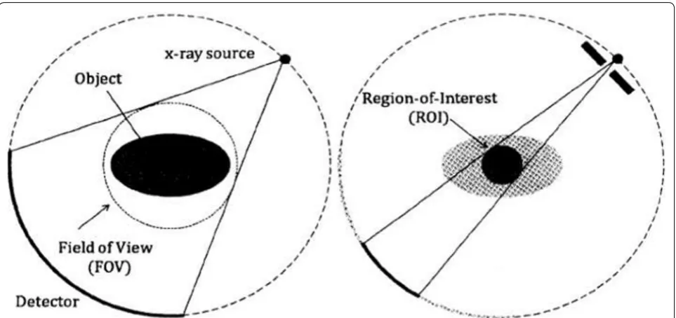
Computed tomography is a permanently evolving X-ray imaging technique finding various applications from medical imaging to materials science and non-destruc-tive testing [1]. From a series of radiographs acquired at various angles, the interior of the scanned volume is reconstructed. In the ideal case, i.e., with a sufficient signal-to-noise ratio and a proper modeling, the recon-struction can be computed relatively easily. However, experimental constraints usually move away from the ideal case and require more advanced reconstruction methods. Among these constraints is the imaging of an object bigger than the detector field of view. This setup is called local tomography or region-of-interest (ROI) tomography.

In local tomography, the detector measures rays com-ing out of the imaged ROI, and also contributions from the external part, as depicted in Fig. 1. As the exter-nal parts are not imaged for every angle, the data are incomplete. This incompleteness is the challenge of local tomography, for it can be shown that the object cannot be stably reconstructed from the acquired data, even in the ROI [2]. The problem of reconstructing a ROI embedded

in a wider object is called the interior problem. The inte-rior problem has infinitely many solutions in general, in the sense that a solution can differ from another solution by an infinitely differentiable function [3].

Local tomography methods basically consist in esti-mating the exterior of the ROI from the acquired meas-urements. This can be done with sinogram extrapolation (see for example [4, 5]) or in the slice domain. These methods, although they can yield satisfactory results, are only heuristics in general. Solutions computed with these methods often suffer from the cupping effect, which is an artifact appearing as a low-frequency bias.

Theoretical investigations, however, found that, with a prior knowledge on region of interest, the interior prob-lem can be solved [6]. This prior knowledge can be about the values of a subregion of the ROI or about the nature of the solution [7, 8].

In this work, we consider a reconstruction method described in [9] where a prior knowledge is available as values of a subregion. We show how the reduction of the number of unknowns can be coupled with an efficient implementation of the involved operators, in order to cope with the scales of modern datasets.

Methods

Based on the observation that the filtered backprojection with extrapolation provides satisfactory reconstruction of medium and high frequencies of the slice, the method

Open Access

*Correspondence: [email protected]

2 _{Université de Grenoble, 11 Rue des Mathématiques,} 38400 Saint‑Martin‑d’Hères, France

aims at improving the reconstructed slice by removing the local tomography artifacts visible as low-frequency artifacts (cupping effect). This correction is performed by representing the reconstruction error in a coarse basis, reducing the number of degrees of freedom of the problem.

From an exact iterative reconstruction method, the reconstruction problem is reformulated to incorporate the local tomography setup, the prior knowledge con-straint and the representation of the image in a coarse basis. Each operator of the forward model is ana-lyzed to enable an efficient implementation. Notably, the projector is reduced to a point-projector which is efficiently implemented with a sparse matrix-vector multiplication.

The local reconstruction implementation is vali-dated on simulated data for which the cupping effect is prominent. The proposed method is compared against another exact local reconstruction method also based on known region. Two criteria are compared: the num-ber of required iterations to achieve an acceptable reconstruction, and the total execution time. The for-mer reflects the relative ill-posedness of the problem and the performance of the chosen optimization algo-rithm, while the latter shows how the efficient imple-mentation of the operators affects the reconstruction time. The benchmarks are carried on data compatible with modern data volumes, up to 40962 pixels with 4000

projections.

An iterative correction algorithm for local tomography

Local tomography and artifacts

The most common local tomography reconstruction method is extrapolating the sinogram before computing the filtered backprojection (FBP), hereafter denoted pad-ded FBP. The extrapolation is usually done by replicating the sinogram boundary values. This prevents truncation artifact (Gibbs phenomenon) from occurring, and often provides acceptable results [10].

However, this technique can fail when the ROI is sur-rounded by anisotropic and/or strongly absorbing mate-rial or when the reconstruction has intrinsically low contrast (for example different parts with the same linear absorption coefficient).

The notable local tomography artifact is the cupping effect. On a reconstructed image, local tomography artifacts appear as a varying contrast. The gray val-ues are typically higher far from the center than close to the center, forming a “cup.” The cupping is also vis-ible when plotting an image line passing through the center, as a function of the pixel location. Such lines are hereby called profiles, for example, the vertical line pro-file is the vertical line of the image passing through the center.

Figure  2 shows the Shepp–Logan phantom with a region of interest. Figure 3 shows the reconstruction with padded FBP, and Fig. 4 shows line profile of the recon-struction. The cupping effect is clearly visible in both the

reconstruction image and profile. This cupping effect can be detrimental for the post-reconstruction analysis, for example, segmentation.

In this work, we examine a family of exact reconstruc-tion methods based on a known subregion. We imple-ment a method handling a reduced number of unknowns by expressing the image in a coarse basis in order to cor-rect the cupping effect.

Iterative reconstruction

Iterative methods in tomography are based on optimi-zation algorithms solving problem (1)

where P is the model of the projection operator, d the acquired data, and x is the unknown volume to recover. In the remainder of this paper, we consider recon-struction of a single slice rather than a volume, so x

shall denote two-dimensional slices. In parallel beam geometry, as it is the case in synchrotrons, reconstruc-tion can be performed by reconstructing the slices independently.

In this context, the reconstructed slice x is an image of support N_×N ₌N2, where N is the number of

pix-els of the detector horizontally. The sinogram d sup-port is N_×Np, where Np is the number of projections.

Thus, the projector is theoretically an operator of dimen-sions (N_×Np, N2), assuming that slices are stacked as

(1)

Px₌d

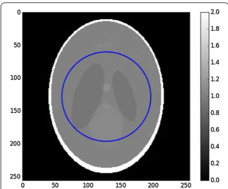
Fig. 2 Shepp–Logan phantom, 2562 pixels. The right bar indicates the gray values, which for real data can be the linear attenuation coef‑ ficient values. The blue circle is the region of interest covered by the detector field of view

one-dimensional N2 vectors, and sinograms are stacked

as one-dimensional N_×Np vectors.

As (1) is ill-posed in general, a surrogate problem is solved instead, for example, problem (2).

where �·�22 is the squared Frobenius norm and φ (x) is a

function bringing stability to the solution. A well-known example of such methods is the Total Variation minimi-zation, which promotes images with sparse gradient.

In local tomography, problem (1) is even more ill-posed due to the incompleteness of the data d, as explained in the introductory part. In order for the solution to be acceptable, the exterior of the ROI has to be estimated. This can be done by extending the support of x to itera-tively estimate the exterior by solving (3)

where x˜ is an image with extended support N2×N2=N22, where N2>N, and P˜ is a wider

projec-tor adapted to this new geometry. To compute the data fidelity term (here the Euclidean distance between P˜x_˜ and d), the size of the projected solution has to be consistent with the acquired data. Thus, the projection is cropped by the means of an operator C to recover the original local geometry. The cropping operator C maps an extended sinogram of support N2×Np to a sinogram of support N_×Np, by keeping only the N central columns. This models the truncation in the local tomography setup, where the detector is not large enough to image the entire object support N2. In practice, the cropping operation is

(2) argmin

x

Px−d

2 2+φ (x)

(3) argmin ˜ x

CP˜x˜−d 2

2+φ (x)˜

implemented inside the projector P˜ by simply restricting

the projection to the detector limited field of view N. In the formulas, the cropping operator C is explicitly sepa-rated from the projector P˜ to highlight the local setup in

the forward model.

Efficient implementations of the projection and back-projection operators enable to solve problem (3). The ASTRA toolbox [11], for example, has versatile geome-try capabilities and built-in algorithms for solving (3) for φ (x)₌0.

In this work, we consider the case where a subregion is known. This prior knowledge on the volume can be used to constrain the sets of solutions. A uniqueness theorem was stated in [6] along with a reconstruction algorithm based on differentiated backprojection and projection onto convex sets to invert the finite Hilbert transform. This algorithm, however, is difficult to imple-ment, and no implementation is readily available for experiments.

We focus on a simpler approach based on formal-ism (3). In this formulation, the prior knowledge can be encoded in several ways. The first is to enforce the values of x˜ in the known region, for example, using an

indica-tor function. The second is to add a term penalizing the distance between the values of x˜ in the known region and

the actual values. We adopt the latter approach, which was proposed, for example, in [12].

Let denote the domain where the values of the vol-ume are known. It is a subset (possibly a union of sub-sets) of the image support N2, and we denote N its

cardinality, that is, the total number of known pixels. Let x_| denote the values of x inside the known region. The

prior knowledge is encoded by φ (x)₌x_|�−u₀

2 2 , where u0 denotes the known values inside and ≥0 is a parameter weighting the fidelity to the known zone. Both x_| and u0 have N components.

Figures 5 and 6 show the reconstruction result on the Shepp–Logan phantom with such choice of φ (x). The cupping effect is almost removed, but the reconstructed slice is also noisy, which is a known effect of least squares minimization on an ill-posed problem when running too many iterations [13]. On the other hand, many iterations are required to reduce the cupping effect.

A workaround on this problem is adding a regu-larization term to stabilize the solution. A popular regularization is Total Variation (TV), promoting piece-wise-constant solutions. The function φ (x) in (3) can then be written φ (x)₌x_|�−u₀

2

2+β�∇x�1, where β_≥0 weights the regularization. Figures 7 and 8 show the result of reconstruction with this method. The recon-struction is much more accurate and bears almost no difference with respect to the ground truth, which is an illustration of the uniqueness theorem stated in [6].

This approach, however, has two drawbacks. The first is using a prior which might not be accurate: in this example, Total Variation promotes piecewise-constant images and is thus not adapted for complex samples. The second draw-back is on the computational side. Adding a non-differenti-able prior involves to change the optimization algorithm for another probably less efficient in the sense that more itera-tions are required to reach convergence. In the examples, the preconditioned Chambolle–Pock algorithm described in [14] was used for the TV minimization. Approximatively, 3000 iterations are required to approximately get rid of the cupping effect (when approximatively 500 are required in the case of a complete scan), and more than 10,000 iterations are required to get the line profiles shown in Fig.  8. This approach is impracticable for modern datasets with increasing amount of data: on the one hand, projection and backprojection become costly operations, while on the other hand, even more itera-tions are required due to the higher number of variables.

The main contribution of this work is an efficient implementation of the method described in [9]. The method is based on the following observation: the pad-ded FBP reconstruction yields acceptable reconstruction of features of the ROI [15], but can suffer from a low-fre-quency bias (cupping effect). On the other hand, iterative algorithms converge slowly due to the high indetermi-nacy of the problem, even with a known subregion. For these reasons, a refinement of the initial reconstruction is computed rather than the complete solution.

Correction of the low‑frequency bias Estimating the reconstruction error

Let x0 be a reconstruction of the region of interest with the padded FBP technique and x♯ be the true values of

the region of interest. Both are slices of support N2

pix-els. The reconstruction error, unknown in practice, is denoted e₌x♯_−x

0. This error mainly consists in low-frequency artifacts (the cupping effect).

In this work, we implement a high-performance ver-sion of algorithm described in [9], aiming at improving an existing reconstruction x0 by removing the cupping effect. This is done by solving the problem described by a new forward model (4)

where xe is a correction term added to the initial reconstruc-tion. Here again, x˜0 denotes an extension of the support of x0, P˜ is a projection operator adapted to this extended geometry, and C is a truncation operator. As the initial reconstruction is constant, problem (4) can be rewritten as

where f ₌d₋CP˜x_˜0. Problem (5) can be understood as fitting the (approximate) reconstruction error f. As the reconstruction error in the ROI is e₌x♯_−x

0, we can write

where x˜♯ _{denotes the whole volume, so that d=CP˜x}˜♯

models the local tomography acquisition. If x0 is extended to x˜0 by inserting zeros, then CP˜x˜0=Px0 as there is no con-tribution from the external part. However, the quantity of interest is the reconstruction error (e) in the ROI, not in the whole volume (e˜). Since the projection of e is different from

the cropped projection of e˜, the term d₋Px0 only approxi-mates the projection of the reconstruction error in the ROI. This quantity is nevertheless used as an approximation of the projection of the reconstruction error in the ROI. Once the optimal correction term xˆe is found, the resulting recon-struction is simply computed as x_{= ˜}C(x_˜0+ ˆxe) where C˜ is

a cropping operator in the image domain, mapping images of support N₂2 to images of support N2.

Reducing the degrees of freedom

The principle of the implemented method is to refine an initial solution of the local tomography problem, knowing that middle and high-frequency features are usually well recovered. By focusing on the low frequen-cies, the complexity of problem (3) can be reduced by solving a simpler problem. Complexity reduction is achieved by expressing the reconstruction error in a coarse basis. (4) argmin xe

CP˜(x˜0+xe)−d 2

2+φ (xe) (5) argmin xe

CPx˜ e−f 2

2+φ (xe)

(6) ˜

e_{= ˜}x♯_{− ˜x} 0 ˜

Pe˜= ˜Px˜♯_{− ˜Px0˜}

CP˜e_˜=d₋Px0

Gaussian function was chosen as a representation basis. The reconstruction error e is estimated by eˆ as a convolution between a finite discrete Dirac comb and a two-dimensional Gaussian function gσ defined by Eq. (7)

where u,v denote discrete indexes in the image, and σ >0 is the standard deviation characterizing the Gauss-ian function. The estimate of the reconstruction error at location (u0,v0), e(uˆ 0,v0), is then given by Eq. (8)

(7) gσ(u,v)₌ 1

σ√2π exp

−u 2_+v2

2σ2

(8) ˆ

e(u0,v0)=

u,v

cu,vgσ(u0−u·s, v0−v·s)

where cu,v are coefficients multiplying the Gaussian func-tions gσ, and s is the spacing (in pixels) between points of the Dirac comb. The summation in (8) actually occurs on a finite support. In our implementation, the Gaussian function is truncated at 3σ at each side, so the sum takes place on a ⌊6σ₊1_{⌋ × ⌊}6σ₊1_⌋ pixels square.

Estimation (8) is done such that projection of ˆe has

minimal Euclidean distance with d₋Px0. Let G denote the operator mapping the coefficients ci,j to the image eˆ

through convolution formula (8). The coefficients vector

c is estimated by solving Problem (9)

(9) argmin

c

CPGc˜ −f 2

2+φ (c)

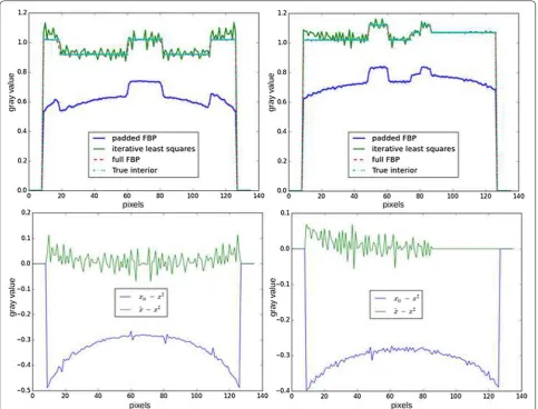
Fig. 6 Line profiles of reconstructions of the Shepp–Logan phantom in a local tomography setup. Top line reconstruction profiles for padded FBP (blue) and iterative least squares (green). Left middle line of the reconstructed image. Right middle column of the reconstructed image. Bottom line

difference profiles between the ground truth x♯ _{and the reconstructions with padded FBP x0 (blue) and iterative least squares xˆ (green). Left middle}

where f ₌d₋Px0 and φ (c) is a constraint function on the coefficients which is detailed later.

Thus, Problem (9) is solved instead of Problem (3). In Problem (9), the unknowns are the coefficients c of the coarse basis. As there are much less coefficients c in the coarse representation than pixels in the extended image support N₂2, the degrees of freedom is accordingly

reduced.

Solving (9) requires the computation of the operators

C, P˜, G, and possibly their adjoints. The implementation

of the crop operator C is straightforward, as it consists in truncating the sinogram to the size of the acquired data. In practice, it consists in modifying the projector P˜ so

that the projections are limited to the reduced detector field of view N2. The operator G can be described as

fol-lows. Coefficients cu,v are placed every s>0 pixel on an image of the size of the extended reconstruction x˜0. This image (a two-dimensional Dirac comb in the continuum case) is then convolved by the kernel gσ. Lastly, an effi-cient implementation of the projection and backprojec-tion operators is needed to solve (9). This is discussed in the implementation section.

Adding the known zone constraint

We now describe how the known zone constraint is implemented in formalism (9). In work [9], the knowl-edge available as known zone values in the slice is trans-lated in the coarse representation basis: a subset of Gaussian coefficients is fitted to values in the known zone ; these coefficients are then used as a constraint for the reconstruction.

In this work, we rather add the constraint directly in the pixel zone. The final optimization problem is

High‑performance implementation

After having reduced the number of degrees of freedom for problem (4), we describe an efficient implementa-tion of the involved operators based on look-up tables (LUTs).

Projection a of Gaussian tiling

The choice of a Gaussian basis for a coarse representa-tion of the correcrepresenta-tion term is based on a characteristic of the Gaussian kernel: it is both rotationally invariant and (10) argmin

c

CPGc˜ −f 2

2+β

Gc_|�−u₀ 2 2

.

Fig. 7 Result of iterative reconstruction with total variation regulari‑ zation. Contrast was adapted with respect to the center of the image

Fig. 8 Line profiles of differences between reconstructions and ground truth. Blue difference between padded FBP x0 and ground truth x♯. Green

difference between iterative total variation minimization xˆ and ground truth x♯_{. Left line profile, right column profile. Total Variation minimization}

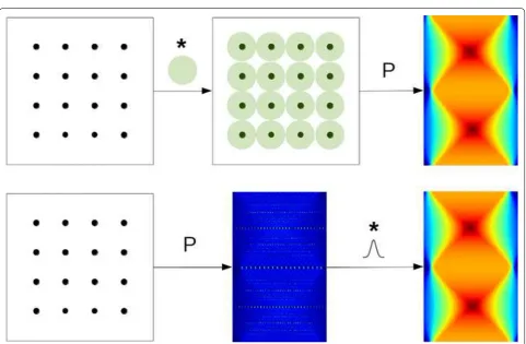
separable [16]. These two properties provide a computa-tional advantage: the order of projection and convolution can somehow be exchanged.

More precisely, given an image y consisting of the Gaussian coefficients evenly placed with a spacing s, the standard way to compute PGy˜ is first performing the

convolution Gy defined by (8) and then projecting with

˜

P. An equivalent computation, however, can be done by

first projecting the image of isolated points y, and then convolving each line of the resulting sinogram by a one-dimensional Gaussian function. This is illustrated in Fig. 9.

This latter approach has two advantages. First, the two-dimensional convolution (or two series of one-dimensional convolution in this separable case) is replaced by a series of one-dimensional convolutions. Secondly, the projection here only consists in pro-jecting isolated points. This operation can be opti-mized by designing a point-projector based on look-up tables.

LUT‑based point‑projector

As previously discussed, the operators involved in for-ward model (10) are a cropping operator, a one-dimen-sional convolution, and a projector. The convolution can be efficiently implemented, either in the Fourier space or in the direct space when one of the functions has a small support. Therefore, a fast projector is essential for solving (10) in an iterative fashion. In our case, the object to pro-ject has a very special structure, as it consists in points spaced by several pixels. Thus, standard projectors of tomography softwares can be replaced by a more efficient implementation, hereby called point- projector, based on look-up tables.

In the remainder, the following notations are used: The support of the original image is N2. The number of

pro-jections is Np, so the acquired sinogram has size N×Np. The size of the extended image is N₂2 where N2≥N. The

number of Gaussian functions used to tile the support is

Ng. The spacing between Gaussian blobs on the image

is s ; thus we have Ng≃

N2 s

2

in a first approximation.

We also use the following indexes convention : Gauss-ian coefficients are numbered with i_{∈ [}0,N_g], and sino-gram indexes are numbered with k_{∈ [}0,Ns] where

Ns=N2×Np is the size of the (extended) sinogram. Each Gaussian coefficient number i_{∈ [}0,Ng[ is

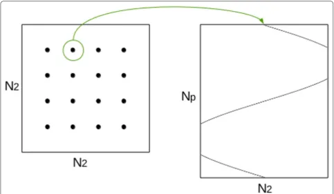
pro-jected on (at most) Np positions in the sinogram. There-fore, a look-up table J is built so that for each i, J[i] is the “list” of locations in sinogram hit by this point after pro-jection. The LUT J is an array of size Ng×Np. Each entry Ji,j corresponds to a position, in the sinogram, that is hit by a projected point i_{∈ [}0,N_g]. For example, entry J0,2 is an index in the sinogram that is hit by point 0 ; and entry J5,j are an indexes hit by point 5 for all j. This is illustrated in Figs. 10, 11.

When computing the sinogram, however, the look-up table J is best accessed “backward”: for a given position

k_{∈ [}0,Ns[ in the sinogram, we have to determine which

points are hitting it through projection. To this end, two look-up tables J and Pos are built. For k_{∈ [}0,Ns], Pos[k]

indicates a position in LUT J, and J_[pk] is a coefficient number i_{∈ [}0,Ng] being projected at position k.

There-fore, the LUT J does not contain sinogram indexes any-more, but rather coefficient indexes. This is illustrated in Fig. 12. The LUT J is re-ordered such that the interval [pk,pk+1−1] gives access to an indexes range in J ; this

index range is the set of all coefficients indexes being pro-jected on sinogram index k.

The point-projector is described by Algorithm  1. The matrix W, indexed in the same way as J, contains the weights of the projections: depending on the position of a point in the image and the projection angle, its projection does not exactly fall into a sinogram pixel. The matrix W

thus encodes the geometric contribution of the projec-tion of the points.

This projection scheme basically consists in stor-ing the explicit projection matrix P˜ with a Compressed

Sparse Row (CSR) format [17], where LUT J corresponds to “col_ind,” LUT Pos corresponds to “row_ptr,” and matrix W contains the values. Storing the entire “linear-algebra” projection matrix without compression would entail to store (N₂2)_×(N2·Np) elements, which is impracticable (for example, more than one terabyte is required for a 10242 slice). However, as each slice point is projected on at most Np sinogram positions, this matrix actually has at most N₂2_×Np non-zero elements. Addi-tionally, as the slice is reduced on a coarse basis, there are N2

s 2

×Np non-zero values to store in this case. The format described above is used to store these elements. Algorithm 1 is thus no more than a matrix-vector multi-plication with a sparse matrix in CSR format.

Fig. 10 Principle of the point‑projector. Gaussian basis coefficients are placed on the image of N2

2 support (left), with even spacing. Each isolated

Algorithm 1Point projector sino: sinogram, of sizeNs=N2×Np

J: LUT, of sizeNg×Np

coeffs: coefficients vector of the Gaussian basis, of sizeNg

W: projection weights, of sizeNg×Np

1:procedurepointProjector(sino, J, coeffs, W) 2: fork∈[0, Ns−1]do

3: pos1 = Pos[k] 4: pos2 = Pos[k+1] 5: forj∈[pos1, pos2[do 6: sino[k] += W[j] * coeffs[J[j]] 7: end for

8: end for 9:end procedure

This approach for computing the point-projector is friendly in a memory-write point of view: after accumu-lating the contributions of all coefficients projected on position k, the sinogram at index k, sino[k], is updated accordingly. This is especially important for GPU imple-mentation, as consecutive threads access contiguous memory locations, which is a coalesced access pattern. On GPUs, each memory transaction actually entails accessing L bytes, so coalesced access to 32 bits scalars results in a read or write of L  /  4 addresses in a single transaction (for example, L=128 for modern NVidia

GPUs).

Implementation of the adjoint operators

As a gradient-based optimization algorithm is used for solving (10), the adjoint of operator CPG˜ has to be

computed. This operator GTP˜TCT consists in

extend-ing the sinogram with zeros, point-backprojectextend-ing and retrieving the Gaussian components from the backprojected image. As mentioned above, the opera-tor G can be described as G=HσU where U is an upsampling operator (here with a factor s), and Hσ is the convolution with 2D Gaussian kernel (7). Thus, GT =H_σTUT which is a downsampling followed by a convolution with kernel (7). The actual computation is then GTP˜TCT =H_σTUTP˜TCT =UTP˜TH_σ1CT where

H_σ1 is a one-dimensional convolution on the sinogram rows.

As previously, these operations can be merged. As

GTP˜TCT returns a Gaussian coefficients vector from

a sinogram, only the coefficients are of interest here. Therefore, the point-backprojector P˜T is merged with the

downsampling UT as previously. For a given coefficient,

we have to find which sinogram entries backproject on the coefficient position. This approach avoids to com-pute useless Ng×(s−1)2 backprojections points on the image, as it is downsampled afterward.

Fig. 11 Illustration of the look‑up table J. The Gaussian coefficients placed on the image are stored in a vector of size Ng (top). Each coeffi‑ cient point (indexed in [0,Ng]) is projected on at most Np positions in

the sinogram. For each i_{∈ [}0,Ng], the structure J[i] =Ji,0,Ji,1,. . . (bottom) contains the list of the sinogram positions hit by projection of i. For example, the Gaussian coefficient number 0 is projected on sinogram positions J0,0,J0,1. . .

Fig. 12 Illustration of the LUT‑based point‑projector. To determine which points are projected on position k∈ [0,Ns] of the sinogram,

The point-backprojector is implemented, as previ-ously, with a LUT J2 of size Ng×Np and a LUT Pos2 of

size Ng+1. The matrix J2 is re-ordered so that for all

i_{∈ [}0,Ng[, the interval [Pos2[i], Pos2[i+1] −1]

corre-sponds to an index range in LUT J2. This is illustrated in

Fig. 13.

The point-backprojector is given by Algorithm  2. Again, the backprojection from a sinogram to a Gaussian coefficients vector corresponds to a matrix-vector mul-tiplication with a matrix in CSR format. The matrix W2 ,

containing the geometric weights of the backprojector, can be viewed as the Column Sparse Storage (CSC) ver-sion of the matrix W.

Algorithm 2Point backprojector

coeffs: coefficients vector of the Gaussian basis, of sizeNg

sino: sinogram, of sizeNs=N2×Np J2: LUT, of sizeNg×Np

W2: backprojection weights, of sizeNg×Np

1:procedurepointBackProjector(coeffs, sino, J2, W2) 2: fori∈[0, Ng−1]do

3: pos1 = Pos2[i] 4: pos2 = Pos2[i+1] 5: forj∈[pos1, pos2[do 6: coeffs[i] += W2[j] * sino[J2[j]] 7: end for

8: end for 9:end procedure

Parallel implementation

In modern experiments carried on X-ray light sources, the data volumes, produced by new generations of detec-tors, always overwhelm the computing power. Simply waiting for more powerful machines is of little hope, as advances in detectors overrun the Moore’s law. Instead, an algorithmic work has to be accomplished to exploit parallelism of modern architectures. In the last decade, the advent of general-purpose GPU (GPGPU) computing was advantageously used, especially in tomography.

The proposed method has been implemented in the PyHST2 software [18] used at ESRF for tomographic reconstruction, with the CUDA language targeting Nvidia GPUs. The point-projector and point-back-projector, which are the most time-consuming opera-tors, are implemented as efficient CUDA kernels. As for Algorithms 1 and 2, the CUDA point-projector and point-backprojector are implemented as matrix-vector multiplication with a matrix in CSR format.

We describe here the implementation of the point-pro-jector, i.e., the computation of the sinogram values sino_[k_] for k_{∈ [}0,Ns]. The point-backprojector follows the same

principle. To compute the sinogram value sino_[k_], the LUT J has to be accessed from pk to pk+1−1 as illustrated in

Fig. 13. This memory range is accessed in parallel by threads of the many-cores GPU with the following principle. Each thread reads m_≥1 values in the LUT. With these values J[j],

where j₌pk,pk+1,. . ., the coefficients vector is accessed

at coeffs_[J_[j_]]. The threads are grouped in blocks, and each thread updates a temporary array in shared memory with the contributions read in coeffs_[J_[j_]]. Then, in each block, the shared array is accumulated by one thread. The result is added to sino_[k_]. This is illustrated in Fig. 14.

The parallelization is done on the read of matrix J, as it is the biggest data structure of the method. As it has been re-arranged so that the interval [pos_[k_], pos_[k₊1_{] −}1_] is a contiguous memory range in J, the described imple-mentation has an efficient memory access pattern.

Multi‑resolution Gaussian basis

The correction term xe in model (4) is a tiling of Gaussian functions : xe=Gc, where c is the vector of coefficients in the Gaussian basis, and G is the operator previously described. In a first approach, all the Gaussian functions (7) have the same variance σ2, so that operator G is linear and problem (10) is convex. The coefficients are placed on a support of size N₂2 before being (theoretically)

con-volved with a 2D Gaussian kernel. The spacing between

Fig. 13 Illustration of the LUT‑based point‑backprojector. To determine which sinogram points are backprojected on coefficient

i_{∈ [}0,Ng], the matrix Pos2 (bottom), is accessed at index i, and

contains the value Pos2_[i_{] =}qi. This value qi is a position in LUT J2

points is s, so that the number of required coefficients is approximately Ng ≃

N2

s 2

.

Another approach is using different variances depending on the position in the image. As only the support N ≤N2

of the original reconstruction x0 has to be corrected, Gauss-ians with a larger support (larger σ) can be used on the

exte-rior of the ROI, further reducing the number of unknowns. By using small Gaussians (small σ) inside the ROI, local

fea-tures can be estimated in the correction term xe, while large Gaussians are used to roughly estimate the contribution of the exterior of the ROI. The new operator G can be written

where σ1,σ2,. . . is a series of standard deviations for the

Gaussians, and Uj are upsampling operators with different factors. This representation is similar to a multi-resolution scheme also used in [19]. This multi-resolution basis allows to further reduce the number of variables in vector c: in this case, Ng <

N2

s 2

. In our implementation, the standard deviations are progressively doubled until reaching the diam-eter of the ROI and then remain constant outside the ROI.

Implementation of (11) is straightforward. The coeffi-cients in vector c are classified according to the distance to the center, forming subsets of coefficients c1_,c2_{,. . . .}

Each subset is point-projected and line-convolved with the corresponding σ1,σ2,. . .. The resulting sinograms are

summed to obtain the projection of Gc.

This representation of correction features as Gaussian blobs is actually not a basis in the mathematical sense: some images cannot be represented by a linear combina-tion of Gaussians. However, this representacombina-tion is very close to a basis for σ _≃s [20]. In our case, we choose s₌0.65_×σ, meaning that there is a significant overlap (11) G₌

j

HσjUj

between the Gaussians. The discrete Gaussian kernel is truncated at 3σ, so its length is _⌈6σ₊1_⌉ samples.

Optimization algorithm

Efficient optimization algorithms can be used to solve the quadratic problem (10). We use the conjugate gra-dient (CG) algorithm, requiring the computation of the adjoint of the involved operators previously described. CG also entails matrix-vector multiplications, which are efficiently implemented with the CSR representation of point-projector and backprojector.

In the GPU implementation, all the involved arrays are single precision (float 32 bits) as most GPUs are relatively not efficient with 64 bits operations. However, the conju-gate gradient algorithm involves scalar products. These operations are implemented by dedicated kernels returning double precision values, as error accumulation is noticeable when accumulating on large arrays in single precision.

Results and discussion

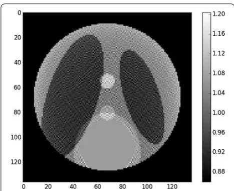
In this section, we compare the proposed method with the basic exact method described in the second section, in term of speed and correction capabilities. The speed benchmarks are done with the low- resolution Shepp– Logan phantom, as the cupping effect is prominent in this image. The setup is illustrated in Fig. 15. The size var-ies in the benchmarks, and the radii of ROI and known zone also vary accordingly. The known zone has been chosen as a uniform zone. In experimental datasets, the known region can be for example regions where the sam-ple contains air, for which the attenuation coefficient is known to be zero.

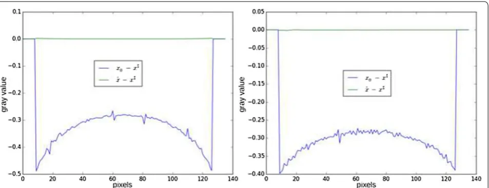
Figure 16 shows the reconstruction results for the setup of Fig. 15. As it can be seen, the cupping effect is mostly removed with respect to the padded FBP technique. Importantly, the proposed method does not create addi-tional artifacts when correcting the cupping effect. Fig-ure 17 shows line profiles of these reconstructions. The known zone constraint provides a reconstruction with an almost zero mean bias.

In the following benchmark, the following notations are used. N is the horizontal size of the initial reconstruc-tion, i.e., the diameter of the acquired ROI, which means that the acquired sinogram has a size N_×Np. N0 is the horizontal size of the whole object support, unknown in practice (for example, N0=512 in the case of the

5122 Shepp–Logan phantom). N2 is the horizontal size

of the extended reconstruction (N2>N), which should

approximate N0. Lastly, Ng is the number of Gaussian

functions used for the proposed method.

All the tests were performed on a machine with a Intel Xeon CPU E5-2643 12 cores 3.40  GHz and a Nvidia Geforce GTX Titan X GPU. As the LUT can be used for

Fig. 14 Illustration of the GPU LUT‑based point‑projector. The memory range [pk,pk+1−1] in LUT J (top, shaded orange) contains

all the indexes needed to be accessed in the coefficients vector to compute sino_[k_]. In this illustration, each thread reads m₌2 values

in the LUT (red rectangles). The threads are grouped in blocks of n

threads (blue rectangles). In the block 1, threads t1,1,. . .,t1,n update

all the slices of a volume, the computation of the LUT is not taken into account. The optimization algorithms used are the preconditioned Chambolle–Pock method [14] for pixel domain exact method and Conjugate Gradient for the proposed method.

We report both the number of iterations needed to converge to the objective function minimum and the total execution time. This gives information on both the efficiency on the optimization algorithm to converge for the given problem and on the complexity of each itera-tion, as the time for one iteration is roughly the total exe-cution time divided by the number of iterations.

Table 1 summarizes the results of the two methods for various setups. For each original phantom size, the two methods are tested with two sets of different parame-ters. For 5122, 10242, 20482, and 40962 original phantom

shapes, the number of projections are, respectively, 800, 1500, 2500, and 4000.

The prototype of [9] was run with the parameters of Table 1. It yields the following execution times: 11.3 s for a 5122 image, 83.1 s for a 10242 image, 842 s for a 20482

image, and 3630 s for a 40962 image. Although it is still

better than the “pixel domain approach,” it suffers from very long execution times for large images.

In the example of 5122 phantom size, the proposed

method is executed with an acquired sinogram of width 272 pixels. The slice is extended to 572 pixels, and the Gaussian basis is configured to have 1345 functions in total. 200 itera-tions yield the reconstruction of Fig. 16 in 10.2 s (without taking the LUT computation time). On the other hand, the standard pixel domain method is executed with 4000 itera-tions and yields a reconstruction similar to Fig. 7, although of slightly lesser quality, in 123 s. The test is then run for a smaller number of Gaussians: the execution time is reduced, but the quality is slightly degraded. This is due to the fact that the number of Gaussians is determined by the spacing

s, which itself is linked to the standard deviation σ.

Decreas-ing the number of unknowns (Ng) speeds up the

computa-tions and also increases the width of the Gaussians, so the reconstruction error might not be appropriately fitted.

The parameters of the proposed method are essentially the size of N2 of the extended slice and the initial value

for σ. As explained in the multi-resolution subsection,

the standard deviations are then progressively doubled until reaching the ROI radius and then kept to a maximal

Fig. 15 Example of local tomography setup on the 5122Shepp– Logan phantom. The outer circle (blue) is the region of interest. The inner circle (green) is the known subregion.

value outside the ROI. Given a size N2, small initial σ

leads to larger computation times as there are more func-tions in the basis, so the LUTs are bigger. Larger initial σ

decreases the computation time but might yield coarser results. Figure 18 shows an example of the influence of the number of Gaussians Ng on the result in the case of

a 10242 _{original phantom. As seeing the profile, the}

cup-ping removal is slightly better when Ng is bigger (smaller

Gaussians), and the error profile is overall closer to zero. The exact method with pixel domain variables starts to be impracticable from 20482 _{pixels slices , as thousands of}

iterations are required to yield an acceptable image qual-ity, leading to hours of processing per slice. The execution times for 40962 _{slices were extrapolated from the}

meas-ured time on 100 iterations: 373 s; therefore, the PSNR are not available in these cases. This method is actu-ally implemented in Python with the ASTRA Toolbox, meaning that only the projection and backprojection are

Fig. 17 Line profiles of reconstructions with the proposed method and the padded FBP. The proposed method was executed with Ng=1345 (left)

and Ng=729 (right), corresponding to a relatively coarser basis.

Table 1 Execution time for various local tomography setups

The columns (N0, N, N2, Ng) describe the problem setup. The next three columns indicate the results for the proposed method. The next three columns indicate the

results for the exact method compared against. The first “Time (s)” column contains the execution time for CPU and GPU, in the form. The second ``Time (s)" column contains the execution time for the other method. Values followed by (E) were extrapolated from previous running times.

N0 N N2 Ng Its Time (s) PSNR Its Time (s) PSNR

512 272 572 1345 200 10.2/2.31 35.5 4000 123 36.79

512 272 572 729 200 5.86/2.01 34.93 3000 106 35.94

1024 544 1144 1345 300 36.71/5.14 28.03 4000 523 31.56

1024 544 1144 2081 300 60.7/11.4 30.25 8000 1094 37.85

2048 1088 2288 1345 500 235/33.5 27.73 4000 3570 15.13

2048 1088 2288 805 500 129/19.2 24.75 7000 6237 20.71

4096 2176 4576 2081 500 1028/109 24.11 4000 14920 (E) N.A.

4096 2176 4576 1037 500 870/97.6 22.74 7000 26110 (E) N.A.

Fig. 18 Line profile of reconstruction of a 10242 _{phantom with 544}2

performed on GPU, so the implementation suffers from memory transfers between CPU and GPU. If fully imple-mented on GPU, one could expect a 5–10 speed-up for this method; nevertheless, the proposed method would still be ahead.

For both methods, the PSNR is progressively decreas-ing as the size of the slice increases, yet the reconstruc-tions are satisfying. We believe this is a consequence of the cupping being not entirely corrected on the slice bor-ders, which brings more and more contribution as the number of pixels increase.

The current GPU implementation provides acceptable speed-up with respect to the CPU implementation, but there is certainly room for improvement as many parts in the CPU implementation are single-threaded. The computation of the LUT takes several minutes for 40962

slices, but the same LUT is re-used for all the slices of a volume.

Conclusion

We proposed a high-performance implementation of a local tomography method aiming at removing the cup-ping effect. The method consists in iteratively correcting an already reconstructed slice and to reduce the recon-struction error in a Gaussian blobs basis. This implemen-tation is based on a careful analysis of the optimization process, showing that the involved operators can be designed especially for this problem.

Results validate the implementation on simulated data, showing that the known zone constraint effectively enforces an almost zero bias. Benchmarks show that

40962 slices can be processed in tens of seconds, making

it able to cope with modern data volumes.

Author details

1 _{ESRF‑The European Synchrotron, 71 avenue des Martyrs, 38043 Grenoble,} France. 2 _{Université de Grenoble, 11 Rue des Mathématiques, 38400 Saint‑Mar‑} tin‑d’Hères, France.

Received: 2 September 2016 Accepted: 9 January 2017

References

1. Herman, G.T.: Fundamentals of Computerized Tomography: Image Reconstruction from Projections. Springer, 233 Spring Street, New York 10013‑1578 (2009)

2. Clackdoyle, R., Defrise, M.: Tomographic reconstruction in the 21st cen‑ tury. IEEE Signal Process. Mag. 27(4), 60–80 (2010)

3. Wang, G., Yu, H.: The meaning of interior tomography. Phys. Med. Biol. 58(16), 161 (2013)

4. Zhao, S., Yang, K., Yang, X.: Reconstruction from truncated projections using mixed extrapolations of exponential and quadratic functions. J. X‑ray Sci. Technol. 19(2), 155 (2011)

5. Van Gompel, G.: Towards Accurate Image Reconstruction from Truncated X‑ray CT Projections. Ph.D Thesis, University of Antwerp, Antwerp (2009) 6. Kudo, H., Courdurier, M., Noo, F., Defrise, M.: Tiny a priori knowledge solves

the interior problem in computed tomography. Phys. Med. Biol. 53(9), 2207 (2008)

7. Yang, J., Yu, H., Jiang, M., Wang, G.: High‑order total variation minimization for interior tomography. Inverse Probl. 26(3), 035013 (2010)

8. Klann, E., Quinto, E.T., Ramlau, R.: Wavelet methods for a weighted sparsity penalty for region of interest tomography. Inverse Probl. 31(2), 025001 (2015) 9. Paleo, P., Desvignes, M., Mirone, A.: A practical local tomography reconstruc‑ tion algorithm based on known subregion. J. Synchrotron Radiat. (2016) 10. Kyrieleis, A., Titarenko, V., Ibison, M., Connolley, T., Withers, P.: Region‑of‑

interest tomography using filtered backprojection: assessing the practical limits. J. Microsc. 241(1), 69–82 (2011)

11. van Aarle, W., Palenstijn, W.J., Beenhouwer, J.D., Altantzis, T., Bals, S., Batenburg, K.J., Sijbers, J.: The ASTRA toolbox: a platform for advanced algorithm development in electron tomography. Ultramicroscopy 157, 35–47 (2015). doi:10.1016/j.ultramic.2015.05.002

12. Rashed, E.A., Kudo, H.: Recent advances in interior tomography. Math. Program. 21st Century Algorithms Model. 1676, 145–156 (2010) 13. Vonesch, C., Ramani, S., Unser, M.: Recursive risk estimation for non‑linear

image deconvolution with a wavelet‑domain sparsity constraint. In: 2008 15th IEEE International Conference on Image Processing, pp. 665–668. IEEE, New York (2008)

14. Pock, T., Chambolle, A.: Diagonal preconditioning for first order primal‑ dual algorithms in convex optimization. In: 2011 International Confer‑ ence on Computer Vision, pp. 1762–1769. IEEE, New York (2011) 15. Bilgot, A., Desbat, L., Perrier, V.: Filtered backprojection method and the

interior problem in 2D tomography (2009)

16. Kannappan, P., Sahoo, P.K.: Rotation invariant separable func‑ tions are Gaussian. SIAM J. Math. Anal. 23(5), 1342–1351 (1992). doi:10.1137/0523076

17. Barrett, R., Berry, M.W., Chan, T.E., Demmel, J., Donato, J., Dongarra, J., Eijkhout, V., Pozo, R., Romine, C., van der Vorst, H.: Templates for the solu‑ tion of linear systems: building blocks for iterative methods vol. 43. SIAM, Philadelphia (1994)

18. Mirone, A., Brun, E., Gouillart, E., Tafforeau, P., Kieffer, J.: The pyhst2 hybrid distributed code for high speed tomographic reconstruction with itera‑ tive reconstruction and a priori knowledge capabilities. Nucl. Instrum. Methods Phys. Res. Sect. B Beam Interact. Mater. Atoms 324, 41–48 (2014). doi:10.1016/j.nimb.2013.09.030

19. Niinimäki, K., Siltanen, S., Kolehmainen, V.: Bayesian multiresolution method for local tomography in dental X‑ray imaging. Phys. Med. Biol. 52(22), 6663 (2007)