M E T H O D O L O G Y
Open Access
A class of continuous bivariate
distributions with linear sum of hazard
gradient components
Jayme Pinto
*and Nikolai Kolev
*Correspondence: [email protected] Department of Statistics, University of São Paulo, São Paulo, Brazil
Abstract
The main purpose of this article is to characterize a class of bivariate continuous non-negative distributions such that the sum of the components of underlying hazard gradient vector is a linear function of its arguments. It happens that this class is a stronger version of the Sibuya-type bivariate lack of memory property. Such a class is allowed to have only certain marginal distributions and the corresponding restrictions are given in terms of marginal densities and hazard rates. We illustrate the methodology developed by examples, obtaining two extended versions of the bivariate Gumbel’s law.
Keywords: Bivariate hazard gradient, Bivariate lack of memory property, Characterization, Gumbel’s bivariate exponential, Marshall-Olkin model, Sibuya’a dependence function
MSC code: Primary: 62H05, 60E05
1 Introduction and motivation
Marshall and Olkin (1967) introduced the classical bivariate lack of memory property (to be denoted byBLMP1) via relation
SX1,X2(x1+t,x2+t)=SX1,X2(x1,x2)SX1,X2(t,t) (1)
for allx1,x2≥0 andt >0, whereSX1,X2(x1,x2)= P(X1 >x1,X2 >x2)is the joint
sur-vival function of non-negative continuous random vector(X1,X2). The functional Eq. (1)
tells us that, independently oft, theBLMP1 preserves the distribution of both(X1,X2)
and its residual lifetime vectorXt=[(X1−t,X2−t)|X1>t,X2>t].
The only bivariate distribution with exponential marginals which possessesBLMP1has
a joint survival function given by
SX1,X2(x1,x2)=exp{−λ1x1−λ2x2−λ3max(x1,x2)}, x1,x2≥0, (2)
whereλi≥0, i=1, 2, 3. The Marshall-Olkin (MO) bivariate exponential distribution (2)
is generated by the stochastic representation
(X1,X2)=[min(T1,T3), min(T2,T3)] , (3)
whereTi are independent and exponentially distributed random variables with
param-eters λi > 0, i = 1, 2, 3. Unlessλ3 = 0, the distribution (2) exhibits singularity along
the linex1 = x2and its contribution toSX1,X2(x1,x2)isα = P(X1 = X2) = λ1+λλ32+λ3,
e.g. Marshall and Olkin (1967). Hence, the MO bivariate exponential distribution is
not absolutely continuous and does not have a probability density with respect to the two-dimensional Lebesgue measure.
Apart from MO bivariate exponential distribution, other known solutions of (1) are the bivariate distributions obtained by Freund (1961), Block and Basu (1974), Proschan and Sullo (1974), Friday and Patil (1977) and all distributions considered by Kulkarni (2006). Consult Chapter 10 in Balakrishnan and Lai (2009) for a related discussion as well.
Johnson and Kotz (1975) introduced another version of the bivariate lack of memory property (the local bivariate lack of memory property), which was rediscovered by Roy (2002) and namedBLMP2. The authors require conditional distributions{X1|X2>x2}
and{X2|X1>x1}to possess (preserve) the univariate lack of memory property. The only
absolutely continuous distribution with such a property is the Gumbel’s type I bivariate exponential distribution given by
SX1,X2(x1,x2)=exp{−λ1x1−λ2x2−θλ1λ2x1x2}, x1,x2≥0 (4)
whereλi>0,i=1, 2 andθ ∈[ 0, 1], see Gumbel (1960). It is negative quadrant dependent
sinceSX1,X2(x1,x2)≤SX1(x1)SX2(x2)for allx1,x2≥0.
If the first partial derivatives ofSX1,X2(x1,x2)exist, one can defineBLMP1andBLMP2
alternatively. We will explore the conditional failure (hazard) rates defined by
ri(x1,x2)= ∂∂ xi
[−lnSX1,X2(x1,x2)] , i=1, 2.
Marshall (1975) and Johnson and Kotz (1975) interpretedri(x1,x2)as the conditional
failure rate of Xi evaluated at xi under condition that Xj > xj fori = 1, 2, i = j.
Equivalently, the conditional hazard rates are the univariate hazard rates of conditional distributions of each variate, given certain inequality of the remainder.
Marshall (1975) named the vectorR(x1,x2) = (r1(x1,x2),r2(x1,x2))the hazard
gradi-ent of the distribution(X1,X2). The hazard gradient vectorR(x1,x2)(if exists) uniquely
determines the bivariate distribution by means of line integral
SX1,X2(x1,x2)=exp
−
CR(z)dz
, (5)
whereCis any sufficiently smooth continuous path beginning at(0, 0)and terminating at(x1,x2). Equation (5) holds provided that along the path of integrationSX1,X2(x1,x2)is
absolutely continuous andR(x1,x2)exists for almost allx1andx2, see Marshall (1975).
The term “almost all” means that the set where the partial derivative does not exist has insignificant measure in the first quadrant, i.e. has a two-dimensional Lebesgue measure zero. See details and a multivariate version in Marshall (1975).
All bivariate distributions which have first partial derivatives and possessBLMP1are
characterized by the equation
r1(x1,x2)+r2(x1,x2)=a0
for almost allx1,x2≥0, wherea0is a non-negative constant, see Theorem 2 in Kulkarni
(2006). In particular, the last relation is valid for the MO bivariate exponential distribution (2) witha0=λ1+λ2+λ3for allx1=x2, since
R(x1,x2)=(r1(x1,x2),r2(x1,x2))= ⎧ ⎪ ⎨ ⎪ ⎩
(λ1+λ3,λ2), ifx1>x2,
does not exist, ifx1=x2,
Thus, the sumr1(x1,x2)+r2(x1,x2) is not defined along the linex1 = x2having a
zero two-dimensional Lebesgue measure. The reason is that the conditional probability
P(Xi>xi|Xj>xj)i,j=1, 2, i=j, experiences a cusp atx1=x2, i.e. it is continuous but
not differentiable atx1 = x2and the corresponding failure rateri(x1,x2)is not defined,
see Singpurwalla (2006), page 99.
In fact, Johnson and Kotz (1975) identifyBLMP2by a local “constancy” of the failure
ratesri(x1,x2), i = 1, 2, see their sections 3(iv) and 5.4. For distribution (4) one gets ri(x1,x2)=λi+a1x3−i, i=1, 2, wherea1is a non-negative constant. Thus, substituting a0 = λ1+λ2anda1 = θλ1λ2, the sum of conditional hazard rates inBLMP2case is
specified by
r1(x1,x2)+r2(x1,x2)=a0+a1x1+a1x2
for allx1,x2≥0.
It would be challenging to linkBLMP1andBLMP2in a new class of bivariate continuous
distributions, to be denoted byL(x;a), satisfying relation
r(x1,x2)=r1(x1,x2)+r2(x1,x2)=a0+a1x1+a2x2 (6)
for almost allx1,x2≥0, wherex=(x1,x2)anda=(a0,a1,a2)is a parameter vector with
non-negative elements, including the possibilitya1=a2.
To show one more member of the classL(x;a), let us consider joint survival function
SX1,X2(x1,x2)=exp −λ1x21−λ2x22−λ3max(x1,x2)
, x1,x2≥0, (7)
which has a singular component along the linex1 = x2 and meets (3). One can verify
that relation (6) is satisfied by settinga0 = λ3 > 0, a1 = 2λ1 > 0 anda2 = 2λ2 > 0.
The distribution given by (7) belongs to the generalized Marshall-Olkin (GMO) distri-butions introduced by Li and Pellerey (2011). The random variablesT1,T2andT3in (3)
are assumed to be independent in the class of GMO distributions, relaxing Marshall-Olkin assumption of exponential marginality. It is direct to check thatSX1,X2(x1,x2) ≥ SX1(x1)SX2(x2)for allx1,x2 ≥0, i.e. the bivariate distribution in (7) is positive quadrant
dependent.
Thus, one can find many examples of bivariate continuous distributions possessing
BLMP1andBLMP2represented by (1) and (4), respectively, as well as those exhibiting
positive or negative quadrant dependence that belong to the classL(x;a) specified by (6). The classL(x;a)is composed of non-negative bivariate distributions which are abso-lutely continuous or continuous with singularity along the lineL = {x1 =x2≥ 0}such
that the sum of the components of underlying hazard gradient is a linear function of both argumentsx1andx2.
It happens that the classL(x;a)(therefore bothBLMP1andBLMP2) is a particular case
of the Sibuya-type bivariate lack of memory property recently introduced by Pinto and Kolev (2015c) as follows.
Definition 1.The non-negative continuous bivariate distribution (X1,X2) with
marginal survival functionsSX1(x1) andSX2(x2) possessesSibuya-type bivariate lack of memory property(to be abbreviated S-BLMP), if and only if
SXt(x1,x2)
SX1t(x1)SX2t(x2)
= SX1,X2(x1,x2) SX1(x1)SX2(x2)
for all x1,x2,t ≥ 0, whereSXt(x1,x2)is the joint survival function of residual lifetime
vectorXtandSXit(xi)are its marginal survival functions,i=1, 2.
The S-BLMP is a new concept. Definition 1 tells us that the random vector(X1,X2)and
its residual lifetime vectorXtshould share, for allt ≥ 0, the same dependence function
DX1,X2(x1,x2)introduced by Sibuya (1960) as follows DX1,X2(x1,x2)=ln
SX1,X2(x1,x2) SX1(x1)SX2(x2)
.
We will refer toDX1,X2(x1,x2)as “Sibuya’a dependence function” hereafter. It exhibits
interesting connections with important cases of dependencies, see Kolev (2016) for related facts.
The article is organized as follows. In Section 2 we first discuss the S-BLMP and justify our attention to its stronger version: the linear Sibuya-type BLMP introduced by Pinto (2014), see Definition 2. We show its equivalence with the class L(x;a) and present characterizations. Naturally, Theorems 1 and 2 are consequences of correspond-ing statements in Pinto and Kolev (2015c). It will be recognized in Section 3 that only certain marginal distributions of the classL(x;a) are allowed. The corresponding con-ditions in terms of marginal densities and hazard rates are presented. Restrictions of
parametersa0,a1 anda2 are given in Theorem 3 and Proposition 1. As a result, one
would be able to generate members of the classL(x;a), some of them being extensions of Gumbel’s law (4), see examples 1A and 3. A discussion and conclusions finalize the paper.
2 A stronger version of S-BLMP
The marginal survival functions of residual lifetime vectorXtare given by
SX1t(x1)=
SX1,X2(x1+t,x2) SX1,X2(t,t)
and SX2t(x2)=
SX1,X2(x1,x2+t) SX1,X2(t,t)
.
Therefore, the relation (8) can be rewritten as
SX1,X2(x1+t,x2+t)=SX1,X2(x1,x2)SX1,X2(t,t)B(x1,x2;t), (9)
for allx1,x2,t≥0, where the continuous functionB(x1,x2;t)= SSXX1t(x1)SX2t(x2)
1(x1)SX2(x2) is such that B(x1,x2; 0)=B(0, 0;t)=1. The functionB(x1,x2;t)is named “aging factor”, see page 457
in Balakrishnan and Lai (2009).
Without some simplifying assumptions onB(x1,x2;t)the class of bivariate
distribu-tions possessing S-BLMP is too cumbersome to be of use. General characterizadistribu-tions of the S-BLMP in terms of functional equations involving Sibuya’s dependence function are presented by Pinto and Kolev (2015c), see their Lemma 1 for example.
In order to get useful models, one should investigate a stronger version of S-BLMP. In this paper we will perform a detailed analysis for a particular aging function of the form
B(x1,x2;t) = exp{−a1x1t−a2x2t}, wherea1anda2are given nonnegative constants.
One can immediately recognize that in addition to relation (8) in Definition 1 one must assume that
SXit(xi)=SXi(xi)exp{−aixit} for ai≥0, i=1, 2. (10)
Definition 2.The non-negative continuous bivariate distribution(X1,X2) possesses linear Sibuya BLMP(to be abbreviated LS-BLMP), if and only if (8) and (10) are satisfied for all x1,x2,t≥0 andai≥0, i=1, 2.
Therefore, the bivariate continuous distributions possessing LS-BLMP can be equiva-lently represented by relation
SX1,X2(x1+t,x2+t)=SX1,X2(x1,x2)SX1,X2(t,t)exp{−a1x1t−a2x2t} (11)
for allx1,x2≥0 andt>0. Really, let (11) be true. Putxi=0 in (11) to get relations (10),
i=1, 2. Substitute the exponent from (10) into (11) to obtain (8). Conversely, let (8) and (10) be fulfilled. Use expression (10) in the left hand side of (8) to restore (11).
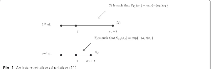
To justify the choice of specific form exp{−a1x1t−a2x2t}of the “aging factor” in (11),
let us consider a system composed by two elements with lifetimes represented by nonneg-ative continuous random variablesX1andX2. Suppose that during the firsttunits of time
the system is protected by breakdowns (by warranty or insurance, say). It is reasonable to assume thatt < min(x1,x2). After those firsttunits of time the system can be affected
by two independent “fatal shocks” governed by homogeneous Poisson processes. Assume finally that thei-th unit is damaged with intensityait, i.e. the corresponding shock arrival
times are exponentially distributed, to be denotedTi∼Exp(ait), i=1, 2, see Fig. 1.
Therefore, the probability of the system survivalSX1,X2(x1+t,x2+t)is given by (11).
Really, the right hand side in (11) is the probabilitySX1,X2(t,t)that both elements survive
the protected initialtunits of time multiplied bySX1,X2(x1,x2)exp{−a1x1t−a2x2t}, being
the probability of absence of shocks during the following xi units of time for thei-th
element,i=1, 2.
The next characterization theorem gives the joint survival function of bivariate contin-uous distributions possessing LS-BLMP.
Theorem 1.The continuous bivariate distribution (X1,X2) has LS-BLMP defined by (11) for all x1,x2 ≥0and t >0if and only if SX1,X2(x1,x2)is a non-degenerate bivariate survival function given by
SX1,X2(x1,x2)= ⎧ ⎪ ⎨ ⎪ ⎩
SX1(x1−x2)exp −a0x2−a1x1x2−
a2−a1
2 x22
, if x1>x2≥0,
exp −a0x1−a1+2a2x21
, if x1=x2≥0,
SX2(x2−x1)exp −a0x1−a2x1x2−
a1−a2
2 x21
, if x2>x1≥0,
(12)
where a0,a1,a2≥0and SXi(xi)are the marginal survival functions, i=1, 2.
Proof. Follows step by step the proof of Theorem 4 in Pinto and Kolev (2015c) with
Ai(x)=aix, i=1, 2.
Theorem 1 tells us that (12) is the solution of the functional Eq. (11).
In Pinto and Kolev (2015c) is also shown that S-BLMP characterizes the distributions belonging to the class defined by relation
r1(x1,x2)+r2(x1,x2)=a0+A1(x1)+A2(x2), (13)
wherea0>0 and the continuous integrable functionsAi(xi)are such thatAi(0)=0 and
Ai(xi) >−a0for allxi>0, i=1, 2.
One can deduce that when B(x1,x2;t) = exp{−a1x1t − a2x2t}, then relation (13)
transforms into (6), i.e.Ai(xi)=aixi, i=1, 2 and we obtain theL(x;a)class.
WhenSX1,X2(x1,x2)is absolutely continuous, its vector hazard gradientR(x1,x2)exists
everywhere in the interior of the set
A= (x1,x2)∈R2+|SX1,X2(x1,x2) >0
,
whereR2+is the first quadrant. In other words, relation (6) is well defined for allx1,x2≥
0. If it happens thatSX1,X2(x1,x2) is continuous, its vector hazard gradientR(x1,x2)is
useful even when it does not exist everywhere in the interior of the setA, see Marshall (1975). Because of possible singularity of the classL(x;a) along the lineLhaving zero two-dimensional Lebesgue measure, we will assume hereafter that first partial derivatives ofSX1,X2(x1,x2)exist and are continuous inA\L.
The next characterization theorem holds for bivariate continuous distributions belong-ing to the classL(x;a)whose survival functions possess continuous first partial deriva-tives, and hence continuous hazard gradient vectorR(x1,x2), inA\L.
Theorem 2.If the first partial derivatives of SX1,X2(x1,x2)exist and are continuous in
A\L, then relation (6) is fulfilled if and only if the joint survival function can be represented by (12).
Proof. Follows step by step the proof of Theorem 2 in Pinto and Kolev (2015c) with
Ai(x)=aix, i=1, 2.
Observe that if our base relation is (11), then the LS-BLMP can be characterized by the joint survival function specified by (12), without the assumption of existence of hazard gradient vectorR(x1,x2)as in Theorem 2.
Applying the Sklar’s theorem to (12), one can obtain the survival copula corresponding to the classL(x;a), see Pinto and Kolev (2015a).
Remark 1. (hazard vector elements in singularity and absolutely continuous cases). The bivariate survival functions considered in Theorem 2 are not necessarily absolutely continuous (and therefore not differentiable inA). In fact, we do not exclude the pos-sibility of existence of a singular component along the lineL = {x1 = x2 ≥ 0}, i.e.
it may happen thatP(X1 = X2) > 0. In such a case, when(x1,x2)belongs to the set
(x1,x2)∈R2+|x1=x2=x
the functionSX1,X2(x1,x2)is not differentiable as well as the
first partial derivatives ofSX1,X2(x1,x2)holds true inA, thenSX1,X2(x1,x2)is absolutely
continuous, see page 357 in Apostol (1974).
If the joint survival functionSX1,X2(x1,x2)isdegenerate(i.e. has degenerate marginal
distributions), from (12) we get
SdeX1,X2(x1,x2)= ⎧ ⎪ ⎨ ⎪ ⎩
exp −a0x2−a1x1x2−a2−2a1x22
, ifx2<x1=const,
exp −a0x−a1+2a2x2
, ifx2=x1=x=const,
exp −a0x1−a2x1x2−a1−2a2x21, ifx1<x2=const.
Obviously,SdeX1,X2(x1,x2)does not have differentiable failure rates.
Now we will identify members of the classL(x;a)with independent marginals. Hence, when(X1,X2)∈L(x;a), we will find solutions of functional equation
SX1,X2(x1,x2)=SX1(x1)SX2(x2) for all x1,x2≥0.
LetrXi(xi)be hazard rates of random variablesXi, i=1, 2. The independence between
X1andX2implies thatri(x1,x2)=rXi(xi), i=1, 2. Therefore, relation (6) transforms into
r(x1,x2)=rX1(x1)+rX2(x2)=a0+a1x1+a2x2.
The last equation is equivalent to both
rX1(x1)=α1+a1x1 and rX2(x2)=α2+a2x2,
whereα1∈[ 0,a0] andα2=a0−α1. Thus, we obtain the following result.
Corollary 1.The vector(X1,X2)with independent marginals belongs the classL(x;a)if and only if the marginal survival functions SXi(xi)have one of the following three possible
analytic forms
exp{−αixi}, exp{−0.5aix2i} or exp{−αixi−0.5aix2i}, i=1, 2,
whereα1+α2=a0withα1∈[ 0,a0]and ai≥0, i=1, 2.
Therefore, the classL(x;a)has only 9 members with independent marginals. It is inter-esting to note that ifSX(x) = exp{−αxi−0.5ax2}, (see the third option in Corollary 1),
thenXhas a linear failure raterX(x) = α1+ax. These type of univariate distributions
have been introduced by Kodlin (1967), see Sen (2006) as well. Additionally, since the two first analytic forms in Corollary 1 can be included in the third one (takingai =0 or
αi=0), the members of the classL(x;a)with independent marginals can also be seen as
an extension of the (univariate) linear hazard rate model to the bivariate setup.
Let us note that the bivariate linear failure distribution introduced by Hangal and Ahmadi (2011) belongs to the classL(x;a).
Finally, one can analyze relation (6) from a completely different point of view. Define the function
ψ(x1,x2)=r(x1,x2)−a0 and set G1(x1)=ψ(x1, 0), G2(x2)=ψ(0,x2).
The linear functionsGi(xi)=aixisatisfy the functional equation
Therefore,Gi(x), i = 1, 2, are additive functionals and only continuous solutions of
Cauchy functional equation f(x + y) = f(x) + f(y), see Theorem 1.1 in Sahoo and Kannappan (2011). In fact, we proved the following statement.
Lemma 1.The class L(x;a) of non-negative bivariate continuous distributions speci-fied by relation (6) can be equivalently defined by linear (additive) functionals G1(x1) = r(x1, 0)−a0and G2(x2)=r(0,x2)−a0, being the only continuous solutions of the Cauchy functional equation f(x+y)=f(x)+f(y).
3 Restrictions on the marginal densities or failure rates
Theorem 2 characterizes bivariate continuous distributions belonging to the classL(x;a), i.e. having joint survival functionSX1,X2(x1,x2) specified by relation (12), which imply
some more restrictions on the margins of these distributions. In other words, the corre-sponding joint survival function is valid only for certain marginal distributions ofX1and X2.
Here we will obtain the associated constraints in terms of marginal densities and hazard rates. As a result, we will get the admissible values of the parameter vectora=(a0,a1,a2).
The methodology will be illustrated by several typical examples.
3.1 Marginal density restrictions
The next statement shows the corresponding parameter constraints in terms of marginal densities whena1+a2>0. The casea1=a2=0, e.g. theBLMP1, is detailed studied by
Kulkarni (2006).
Theorem 3. Let Xibe a random variable with absolutely continuous density fXi(xi), i=
1, 2.Let a0,a1,a2 ≥0and a1+a2 > 0.Then SX1,X2(x1,x2)in (12) is a proper bivariate survival function if and only if
A(xi,xj)−aixj+
d dxi
logfXi(xi−xj)+ai[xjA(xi,xj)−1]
SXi(xi−xj)
fXi(xi−xj)
≥0 (14)
where A(xi,xj)=a0+aixi+(aj−ai)xjfor all xi≥xj≥0, i=j, i,j=1, 2.The singularity
contribution into the joint survival function is given by
α=P(X1=X2)=
fX1(0)+fX2(0)−a0
π
2(a1+a2) ×exp
a20
2(a1+a2)
1−Erf
a0 √
2(a1+a2)
,
(15)
where Erf(x) = √2
π
x
0 exp{−t2}dt. In addition, the survival function specified by (12) is absolutely continuous if and only if fX1(0)+fX2(0)=a0.
Proof. LetSX1,X2(x1,x2)be given by (12). Then, it is a proper if
∂2
∂x1∂x2
SX1,X2(x1,x2)≥0,
After some algebra the last condition transforms into inequality (14).
Since SX1,X2(x1,x2) may have a singular component along the line x1 = x2, then
proper if and only if both the absolutely continuous partSacX1,X2(x1,x2)and the singular
partSsiX1,X2(x1,x2)are survival functions and SX1,X2(x1,x2)=(1−α)SacX1,X2(x1,x2)+αS
si
X1,X2(max{x1,x2})
forα∈[0, 1]. An equivalent expression in terms of joint densities is given by
fX1,X2(x1,x2)=(1−α)f
ac
X1,X2(x1,x2)+αf
si
X1,X2(max{x1,x2}),
where
(1−α)fXac1,X2(x1,x2)= ∂ 2
∂x1∂x2
SX1,X2(x1,x2).
To ensure existence ofSX1,X2(x1,x2)we should evaluate the probabilityαwhich is
equiv-alent to impose that 1−α =P(X1>X2)+P(X2>X1) ∈[ 0, 1] , so one has to calculate
the probabilities in the last sum. We have
P(X1>X2)= ∞
0 u
0 (
1−α)fXac1,X2(u,v)dvdu.
Computing the inner integralI(u)=0u(1−α)fXac1,X2(u,v)dvwe get
I(u)= −fX1(0)exp
−a0u−
a2+a1
2 u
2
−a1uexp
−a0u−
a2+a1
2 u
2
+fX1(u).
Therefore,
P(X1>X2)= ∞
0 I(u)du = −fX1(0)
∞
0 exp −a0u− a2+a1
2 u2
du−a1 ∞
0 uexp −a0u− a2+a1
2 u2
du+1. (16)
In order to solve integrals in (16), we use the following two expressions taken from Gradshteyn and Ryzhik (2007) for positive constantscandd:
∞
0
exp{−cu2−du}du= 1
2 π c exp d2
4c 1−Erf
d
2√c
,
(see equation 3.322.2 on page 336), and
∞
0
uexp{−cu2−du}du= 1
2c− d 4c π c exp d2
4c 1−Erf
d
2√c
,
(see equation 3.462.5 on page 365). Substitutingc= a1+a2
2 andd=a0we obtain from (16)
P(X1>X2)= a2 a1+a2 −
fX1(0)−
a0a1 a1+a2
π
2(a1+a2)
exp
a20
2(a1+a2)
×
1−Erf
a0 √
2(a1+a2)
.
In a similar way we get
P(X2>X1)= a1 a1+a2 −
fX2(0)−
a0a2 a1+a2
π
2(a1+a2)
exp
a20
2(a1+a2)
×
1−Erf
a0 √
2(a1+a2)
From the last expressions and (16) we arrive to (15). To conclude the proof, observe that
SX1,X2(x1,x2)in (12) is absolutely continuous if and only ifα =0, which is equivalent to
required conditionfX1(0)+fX2(0)=a0.
Notice that if inequality (14) is fulfilled for somea0=u>0, then it is also satisfied for
alla0≥u. Denote by
τ =the greatest lower bound of the set of possible values ofa0satisfying(14).
Depending on the marginal densities, it may happen in some special cases thatτ >
fX1(0)+fX2(0), which contradicts (15) since alwaysα = P(X1 = X2) ≥ 0, i.e.a0 ≤ fX1(0)+fX2(0). Such highτ-values would be outside of the parameter spaceAof the class
L(x;a).
The range of possible values of a0 are shown in Proposition 1. It is crucial for the
construction of proper bivariate survival functions belonging to the classL(x;a) from pre-specified marginal densities as we will see later.
Proposition 1.Supposeτ ≤fX1(0)+fX2(0).If a0∈
max{τ, max(fX1(0),fX2(0))},fX1(0)+fX2(0)
, (17)
then Theorem 3 is fulfilled.
Proof. In the absence of singularity (wheneverα = P(X1 = X2) = 0), one concludes
from (15) thatfX1(0)+fX2(0)−a0= 0. Therefore, alwaysa0≤fX1(0)+fX2(0), which is
the upper bound fora0in (17).
The increase of the singular contribution intoSX1,X2(x1,x2)implies increasing of the
probabilityα=P(X1=X2)up to 1. Let us denote by E(a0,a1,a2)=a0
π
2(a1+a2)
exp
a20
2(a1+a2)
1−Erf
a0 √
2(a1+a2)
.
It is direct to check that 0≤E(a0,a1,a2)≤1. We may represent (16) as P(X1>X2)=1−
fX1(0) a0
E(a0,a1,a2)− a1 a1+a2
[ 1−E(a0,a1,a2)] .
The right hand side of the last equation is non-negative iffX1(0)≤a0. By analogy, from
the expression forP(X2>X1)we obtainfX2(0)≤a0.
Notice that ifa0∈[ max{fX1(0),fX2(0)},fX1(0)+fX2(0)] thenα∈[ 0, 1] . Finally, the lower
bound in (17) can be obtained by taking into account the restriction ona0imposed by
inequality (14) and possible relatedτ−values.
Remark 2. (absolutely continuous rule).Observe that whenever the upper boundaUfor
a0given by (17) is attainable, i.e. ifaU = a0 = fX1(0)+fX2(0), one obtains an
abso-lutely continuous bivariate distribution for which (6) is valid. Therefore, Eq. (15), besides representing the constrainta1+a2 > 0, also offers a way to identify the presence of
singularity.
0, or equivalently, whenrX1(0) = rX2(0) = 0, indicating thata0= 0. For example,
con-sider a joint distribution given bySX1,X2(x1,x2)=exp{−0.5a1x21−0.5a2x22}. Observe that
bothfX1(0) =fX2(0) = 0 implyinga0 =0 andα =P(X1= X2)= 0. This special
abso-lutely continuous bivariate distribution with independent marginals case may be treated as an “exception”, compare with Corollary 1.
Finally, note that all members of the class L(x;a) with independent marginals are absolutely continuous.
Remark 3. (singularity of the BLMP1models).In the particular casea1 = a2 = 0, the
condition (14) transforms into inequality (ii) of Theorem 5.1 in Marshall and Olkin (1967). In addition, the possible interval values ofa0in (17) are compatible with those given by
Kulkarni (2006) in her Remark 1.
Remark 4. (singularity of the GMO models).Let us consider the joint survival function of
(Y1,Y2)belonging to the class of GMO distributions and represented by (7), withai=2λi,
i=1, 2, andλ3=a0. It is direct to check that
P(Y1=Y2)=a0
π
2(a1+a2)
exp
a20
2(a1+a2)
1−Erf
a0 √
2(a1+a2)
.
Observe that the right hand side in the last equation is just the functionE(a0,a1,a2)
used in the proof of Proposition 1.
We noted in the proof of Theorem 3 that if the survival functionSX1,X2(x1,x2)given
by (12) is proper then ∂x∂2
1∂x2SX1,X2(x1,x2) should be non-negative. This condition is
equivalent to the requirement
SX1,X2(x1,y1)+SX1,X2(x2,y2)−SX1,X2(x1,y2)−SX1,X2(x2,y1)≥0
for any two points(x1,y1)and(x2,y2)inR2+such thatx1≤x2andy1≤y2. For example,
ifx1≤x2≤y1≤y2anda2=0 we conclude from (12) that the last inequality regarding
the joint survival function is equivalent to
SX2(y1−x1)−SX2(y2−x1) SX2(y1−x2)−SX2(y2−x2)
≤exp
−(x2−x1)
a0+ a1
2 (x2+x1)
.
In general, such constraints between marginal survival functions are not easily verified. Relations (14) and (15) in Theorem 3 give alternative conditions in terms of absolutely continuous marginal densitiesfXi(x),i= 1, 2. However, depending on the complexity of
the analytical form of the densities involved, it may be difficult to check these restrictions.
3.2 Marginal failure rates restrictions
The next result offers another set of equivalent constraints for parameters ofL(x;a), but in terms of marginal failure ratesrXi(x), i=1, 2.
Theorem 4.Let the marginal failure rates rXi(x),i = 1, 2,be differentiable functions
0≤rXi(xi)≤a0+aixi; (18a)
rXi(xi−xj)[A(xi,xj)−aixj−rXi(xi−xj)]
+ d
dxi
rXi(xi−xj)+ai[xjA(xi,xj)−1]≥0,
(18b)
with A(xi,xj)=a0+aixi+(aj−ai)xj,for xi≥xj≥0,i,j=1, 2,i=j;
a0∈
max{τ, max(rX1(0),rX2(0))},rX1(0)+rX2(0)
, (18c)
whereτ denotes the greatest lower bound of the set of values of a0for which the inequality (18b) is satisfied.
Then the joint survival function SX1,X2(x1,x2)given by (12) is proper with marginals SXi(xi) = exp
−xi
0 rXi(u)du
, xi ≥ 0,i = 1, 2. The joint distribution is absolutely
continuous if and only if a0=rX1(0)+rX2(0), otherwise it possesses a singular component. Proof. LetSX1,X2(x1,x2)be given by (12) and let the univariate failure ratesrXi(xi) be
differentiable functions,i=1, 2. Suppose thatx2≥x1≥0. Then substitutingx1=0 in
r1(x1,x2)=
rX1(x1−x2)+a1x2, ifx1>x2≥0, a0+(a1−a2)x1+a2x2−rX2(x2−x1), ifx2>x1≥0
one getsr1(0,x2)=a0+a2x2−rX2(x2)≥0 and thereforerX2(x2)≤a0+a2x2. By analogy,
we conclude thatrX1(x1)≤a0+a1x1ifx1≥x2≥0 and (18a) is established.
All other relations are consequence of Theorem 3.
Conditions (18a), (18b) and (18c) in Theorem 4 imply several simple practical steps that help to fix the permissible parameter space of coefficientsa0,a1anda2 inL(x;a). We
discuss them in the next remark.
Remark 5. (parameter space of the classL(x;a)).Inequality (18a) says that the bivariate distributions from the classL(x;a)satisfying (6) cannot have marginal distributions with failure ratesrXi(xi)above the linea0+aixi fori = 1, 2. For example, distributions with
univariate failure rate of the formax2i, fora>0 are unable to meet (6). In addition, sincerXi(.)is a failure rate, then
∞
0 rXi(u)du= ∞and because of (18a) the
support ofXi,i= 1, 2, cannot be bounded from above, i.e. has to be the entire half line
[ 0,∞).
To summarize, the parameter space for the coefficientsa0,a1anda2satisfying (6) in
terms of marginal failure rates is given by
{a0∈max{τ, max(rX1(0),rX2(0))},rX1(0)+rX2(0)
, a1,a2≥0, a1+a2>0},
becauserXi(0)=fXi(0)fori=1, 2. Finally, note that admissible values for coefficientsa1
anda2may be further limited as a consequence of inequality (18b) from Theorem 4, see
The converse of Theorem 4 also holds for non-degenerate distributions and the statement is given below.
Proposition 2.If SX1,X2(x1,x2)is non-degenerate bivariate survival function given by Eq. (12) and has differentiable marginal failure rates then it must satisfy conditions (18a) to (18c) in Theorem 4.
Proof.Follows step by step the proof of Proposition 1 in Kulkarni (2006).
The rules established in Theorem 4 may serve as a useful guide for constructing bivariate distributions possessing property (6). The building scheme may be relaxed under additional available information regarding monotone behavior of marginal failure rates. In fact, the class of bivariate distributions L(x;a) may have arbitrary combina-tion of marginal failure rates: increasing, decreasing, constant, bathtub, etc., implying corresponding restrictions for the parameter space, of course.
3.3 Examples
The next two examples illustrate how relations in Theorem 4 can be applied to construct bivariate distributions fromL(x;a)with given marginal failure rates.
Example 1. (constant failure rate marginals).Assume that
SXi(x)=exp{−λix}, i.e. Xi∼Exp(λi) λi >0, i=1, 2.
ThenfXi(x)= λiexp{−λix},rXi(x)=λiandfXi(0)=rXi(0)= λi, i= 1, 2. From (18c)
we obtain the first restriction: max(λ1,λ2)≤a0≤λ1+λ2.
Letx1≥x2. Sincea1≥0, inequality (18b) transforms into
0≤a1≤(λ1+a1x2)[a0−λ1+a1(x1−x2)+a2x2] ,
for allx1 ≥ x2 ≥ 0. The function(λ1+a1x2)[a0−λ1+a1(x1−x2)+a2x2] is
non-decreasing and its minimum is equal toλ1(a0−λ1)whenx1 =x2= 0. Therefore, 0 ≤ a1≤λ1(a0−λ1).
To find the greatest lower boundτ for which condition (18c) in Theorem 4 is true, is
equivalent to verify whenλ2(a0−λ2)+λ2a0a1x2+λ2a0a1x22≥0. The last inequality is
satisfied whena0≥λ2. But we got this lower bound fora0already.
Analogously, whenx2≥x1we obtain 0≤a2≤λ2(a0−λ2).
Summarizing, the parameter space is
max(λ1,λ2)≤a0≤λ1+λ2, a1+a2>0 and 0≤ai≤λi(a0−λi), i=1, 2.
We will consider two possible cases:
1A.The bivariate survival function will be absolutely continuous ifa0=λ1+λ2. Hence, ai =θiλ1λ2forθi ∈(0, 1] ,i=1, 2. With these specific parameters we get from (12) the
representation
SX1,X2(x1,x2)= ⎧ ⎨ ⎩
exp
−λ1x1+λ2x2+λ1λ2x2(θ1x1+θ2−2θ1x2)
, ifx1≥x2,
exp−λ1x1+λ2x2+λ1λ2x1(θ2x2+θ1−2θ2x1)
, ifx2≥x1,
which may be namedGeneralized Gumbel’s bivariate exponential distribution.
Observe, that fixingθ1 = θ2 =θ in the last relation we obtain as a particular case the
Gumbel’s type I bivariate exponential distribution (4).
1B.A bivariate survival function with absolutely continuous and singular components
can also be constructed whena0 < λ1+λ2. Supposeλ1 > λ2and leta0 = λ1. Notice
that with this parameter choice the restrictions in (18c) are fulfilled. Hence we obtain
a1=0 anda2=θλ2(λ1−λ2), whereθ ∈(0, 1] . Substituting these parameter values in
(12) we get
SX1,X2(x1,x2)= ⎧ ⎪ ⎪ ⎪ ⎨ ⎪ ⎪ ⎪ ⎩ exp
−λ1x1+θλ2(λ21−λ2)x22
, ifx1≥x2,
exp{−[(λ1−λ2)x1+λ2x2]} ×exp−θλ2(λ1−λ2)x1(x2−
x1
2)
, ifx2≥x1.
In what follows, we will build a bivariate distribution with increasing marginal failure rates.
Example 2. (increasing failure rate marginals).Consider
SXi(x)=exp −λix
2−λ 3x
for x≥0,λi>0,λ3>0, i=1, 2.
SincefXi(x) = (2λix+λ3)exp −λix2−λ3x
, thenrXi(x) = 2λix+λ3,i = 1, 2, and
the marginals have increasing failure rate. First limitations on the parameter space come from inequalities (18a) and (18c), i.e.a0≥λ3andai≥2λi,i=1, 2.
Whenx1≥x2≥0, from (18b) we get a nonnegative increasing inx1andx2function
2λ1−a1−[ 2λ1(x1−x2)+λ3+a1x2] [(2λ1−a1)(x1−x2)+λ3−a0−a2x2]≥0
with a minimum at the point(0, 0). Hence we obtaina1≤2λ1+λ3(a0−λ3).
Analogously, forx1≥x2≥0, we get 2λ2≤a2≤2λ2+λ3(a0−λ3).
Summarizing, we have the constraints
λ3≤a0≤2λ3and 2λi≤ai≤2λi+λ3(a0−λ3), i=1, 2.
2A.Ifa0=2λ3we obtain an absolutely continuous bivariate survival function. In this
caseai=2λi+θiλ23,θi∈[ 0, 1] ,i=1, 2 and letting these values in (12) one gets
SX1,X2(x1,x2)= ⎧ ⎪ ⎪ ⎪ ⎪ ⎪ ⎪ ⎪ ⎪ ⎪ ⎪ ⎨ ⎪ ⎪ ⎪ ⎪ ⎪ ⎪ ⎪ ⎪ ⎪ ⎪ ⎩
exp −λ1x21+λ3x1+λ2x22
×exp
−
λ3x2+λ23x2(θ1x1+θ2−θ1
2 x2)
, ifx 1≥x2,
exp −λ2x22+λ3x2+λ1x21
×exp
−
λ3x1+λ23x1(θ2x2+θ1−θ2
2 x1)
, ifx 2≥x1.
Observe that the expression of the joint survival function involves a complete
sec-ond degree polynomial in the exponent. In addition, notice thatθ1 = θ2 = 0 implies
independence betweenX1andX2.
2B.A bivariate survival function having absolutely continuous and singular component
can also be captured substituting
in (12). Letθ0=0 in the corresponding expression to get relation (7), i.e the distribution
from the class of GMO distributions, see Li and Pellerey (2011).
Example 3. (“min” operation based construction).Let the survival function of the bivari-ate random vector(Y1,Y2)follow Gumbel’s type I bivariate exponential distribution given
by (4) which is a member of the classL(x;a). Assume thatY3∼ Exp(λ3)is independent
of(Y1,Y2). Therefore,(X1,X2)=[ min(Y1,Y3), min(Y2,Y3)] belongs toL(x;a)as well and
its survival function is given by
SX1,X2(x1,x2)=
exp{−(λ1+λ3)x1−λ2x2−θλ1λ2x1x2}, ifx1≥x2,
exp{−λ1x1−(λ2+λ3)x2−θλ1λ2x1x2}, ifx2≥x1.
(20)
Notice thatSY1,Y2(x1,x2)is absolutely continuous, butSX1,X2(x1,x2)displays a singular
component along the linex1=x2. The expression (20) is given by Pinto and Kolev (2015c)
in their Example 1.
It is worth noting that SX1,X2(x1,x2) given by (20), despite being continuous (but
not absolutely continuous), preserves the local constancy of the failure ratesr1(x1,x2)
andr2(x1,x2) in a very similar fashion as Gumbel’s bivariate distribution (4) does, i.e. ri(x1,x2)=λi+a1x3−i, i=1, 2,. The hazard components of (20) are given by
ri(x1,x2)= ⎧ ⎪ ⎨ ⎪ ⎩
λi+λ3+θλ1λ2x3−i, ifxi>x3−i,
does not exist ifx1=x2,
λi+θλ1λ2x3−i, ifxi<x3−i
fori=1, 2. Therefore, we may consider (20) as aGumbel’s extended bivariate exponential distribution with a singularityalong the linex1=x2. Substitutingλ3=0 in (20), one will
get absolutely continuous Gumbel’s version (4).
Remark 6. (expanding Gumbel’s bivariate law).The construction in Example 3 incorpo-rates a singular component into the resulting distribution, which belongs to a wider class of Extended Marshall Olkin (EMO) bivariate distributions introduced by Pinto and Kolev (2015b). In fact, we assume thatT1andT2are dependent random variables, but
indepen-dent ofT3in stochastic representation (3). Particular members of the EMO-class are the
MO bivariate exponential distribution satisfying (3) and the GMO distributions (remind that the joint distribution given by (7) is member of the GMO-class).
4 Discussion and conclusions
In this paper we study a stronger version of S-BLMP introduced by in Pinto and Kolev (2015c), see Definition 1. We define the classL(x;a)and characterize it by the following equivalent relationsL(x;a)⇔(6)⇔(12). In addition,
Lemma 1⇔L(x;a)⇔LS−BLMP⇔(11).
Thus, the classL(x;a)might be treated as a key tool to deepen the BLMP-notion giv-ing possibility to model the aggiv-ing phenomena in the complement to the “non-aggiv-ing”
one, which fixes the world on Eqs. (1) or (4), viaBLMP1andBLMP2correspondingly.
dependent; distributions from the GMO and EMO classes, etc. This huge variety of bivariate distributions would help to choose the “right” model consistent with the phys-ical nature of the observations. The selection of bivariate distribution to be used should depend on considerations involving both the physical scenario at hand, and the properties of chosen distribution.
The seminal Gumbel’s type I bivariate exponential distribution given by (4) has a central place in probability theory, being object of many characterization results. To count several of them, it is: the only absolutely continuous bivariate distribution possessingBLMP2;
belongs to the classL(x;a); a key bivariate extreme value distribution, etc. We got two extensions of the Gumbel’s type I distribution: one being absolutely continuous and the other having a singular component, represented by (19) and (20) respectively, consult Remark 6 as well. We do believe that further characterizations based on those relations will elevate the generalized Gumbel’s laws as a starting point and a base for obtaining new bivariate models, with higher flexibility and chances to better model the genuine dependence structure.
We did not consider in this article inference procedures related to the model (6), nor its application for real data set. But, in Pinto and Kolev (2015b) we perform a Bayesian analysis using the EMO distribution (20) (being a member of the classL(x;a)) for a soccer data with ties studied by Meintanis (2007) and many other authors. According to the Deviance Information Criterion, our model (20) presented better fit than the Marshall-Olkin bivariate Weibull distribution, recently introduced by Kundu and Gupta (2013), who analyzed the same data set.
In general, one may use techniques for estimation of bivariate density function with par-tially differentiable kernels, e.g. Scott (1992). Another option is to apply the Kaplan-Meier estimate of bivariate survival function, even in the case of censoring following Dabrowska (1988), for example. Once the model is selected, goodness of the fit can be tested with conventional methods.
Acknowledgments
The authors are grateful to the Editors and the referees for their suggestions which helped to improve this article. The first author is grateful for the support of the Central Bank of Brazil. The second author is partially supported by FAPESP (2013/07375-0) and TUBITAK grants.
Received: 11 April 2016 Accepted: 10 May 2016
References
Apostol, TM: Mathematical Analysis. 2nd Edition. Addison-Wesley, Reading (1974)
Balakrishnan, N, Lai, C-D: Continuous Bivariate Distributions. 2nd Edition. Springer, New York (2009) Block, HW, Basu, AP: A continuous bivariate exponential extension. J. Am. Stat. Assoc.69, 1031–1037 (1974) Dabrowska, D: Kaplan-Meier estimate on the plane. Ann. Stat.16, 1475–1489 (1988)
Freund, E: A bivariate extension of the exponential distribution. J. Am. Stat. Assoc.56, 971–977 (1961)
Friday, DS, Patil, GP: A bivariate exponential model with applications to reliability and computer generation of random variables. In: Tsokos, CP, Shimi, IN (eds.) The Theory and applications of Reliability, vol. 1, pp. 527–549. Academic Press, New York, (1977)
Gradshteyn, IS, Ryzhik, IM: Tables of Integrals, Series and Products. 7th Edition. Academic Press, Boston (2007) Gumbel, E: Bivariate exponential distributions. J. Am. Stat. Assoc.55, 698–707 (1960)
Hangal, D, Ahmadi, K: Bivariate linear failure distribution. Int. J. Stat. Manag. Sci.6, 73–84 (2011) Johnson, NL, Kotz, S: A vector multivariate hazard rate. J. Multivariate Anal.5, 53–66 (1975) Kodlin, D: A new response time distribution. Biometrics.23, 227–239 (1967)
Kolev, N: Characterizations of the class of bivariate Gompertz distributions. J. Multivariate Anal.148, 173–179 (2016) Kulkarni, HV: Characterizations and modelling of multivariate lack of memory property. Metrika.64, 167–180 (2006) Kundu, D, Gupta, A: Bayes estimation for the Marshall-Olkin bivariate Weibull distribution. Comput. Stat. Data Anal.57,
271–281 (2013)
Marshall, AW: Some comments on the hazard gradient. Stoch. Process. Appl.3, 293–300 (1975) Marshall, AW, Olkin, I: A multivariate exponential distribution. J. Am. Stat. Assoc.62, 30–41 (1967)
Meintanis, S: Test of fit for Marshall-Olkin distributions with applications. J. Stat. Plann. Infer.137, 3954–3963 (2007) Pinto, J: Deepening the Notions of Dependence and Aging in Bivariate Probability Distributions. PhD Thesis. Sao Paulo
University Press, Sao Paulo (2014)
Pinto, J, Kolev, N: Copula representations for invariant dependence functions. In: Glau, K, Scherer, M, Zagst, R (eds.) Innovations in Quantitative Risk Management, vol.99, pp. 411–421. Springer Series in Mathematics & Statistics, Springer Heidelberg, (2015a)
Pinto, J, Kolev, N: Extended Marshall-Olkin model and its dual version. In: Cherubini, U, Durante, F, Mulinacci, S (eds.) Marshall-Olkin Distributions - Advances in Theory and Applications, vol. 141, pp. 87–113. Springer Series in Mathematics & Statistics, Springer Heidelberg, (2015b)
Pinto, J, Kolev, N: Sibuya-type bivariate lack of memory property. J. Multivariate Anal.134, 119–128 (2015c)
Proschan, F, Sullo, P: Estimating the parameters of a bivariate exponential distribution in several sampling situations. In: Proschan, F, Serfling, RJ (eds.) Reliability and Biometry: Statistical Analysis of Life Lengths, pp. 423–440. Society of Industrial and Applied Mathematics, Philadelphia, (1974)
Roy, D: On bivariate lack of memory property and a new definition. Ann. Inst. Stat. Math.54, 404–410 (2002) Sahoo, PK, Kannappan, P: Introduction to Functional Equations. CRC Press, Boca Raton (2011)
Sen, A: Linear failure rate distributions. In: Kotz, S, Read, C, Balakrishnana, N, Vidakovic, B (eds.) Encyclopedia of Statistical Sciences. 2nd ed, pp. 4212–4217. Wiley, New Jersey, (2006)
Scott, D: Multivariate Density Estimation: Theory, Practice and Visualization. Wiley, New York (1992) Sibuya, M: Bivariate extreme statistics I. Ann. I.st. Stat. Math.11, 195–210 (1960)
Singpurwalla, N: Reliability and risk: a Bayesian perspective. Wiley, Chichester (2006)
Submit your manuscript to a
journal and benefi t from:
7Convenient online submission
7Rigorous peer review
7Immediate publication on acceptance
7Open access: articles freely available online
7High visibility within the fi eld
7Retaining the copyright to your article