Optic flow based perception of two-dimensional
trajectories and the effects of a single landmark.
R.J.V. Bertin, I. Israël
Collège de France / L.P.P.A. 11, place Marcelin Berthelot 75005 ParisFrance
✆
fax:
Optic flow based perception of two-dimensional
trajectories and the effects of a single landmark.
R.J.V. Bertin, I. Israël
Abstract
It is well established that human observers can detect their heading direction on a very short time scale on the basis of optic flow (500ms; Hooge et al., 2000). Can they also integrate these perceptions over time to reconstruct a 2D trajectory simulated by the optic flow stimulus? We investigated the visual perception and reconstruction of passively travelled two-dimensional trajectories from optic flow with and without a single landmark. Stimuli in which translation and yaw are unyoked can give rise to illu-sory percepts; using a structured visual environment instead of only dots can improve perception of these stimuli. Does the additional visual and/or extra-retinal information provided by a single land-mark have a similar, beneficial effect? Here, seated, stationary subjects wore a head-mounted display showing optic flow stimuli that simulated various manoeuvres: linear or curvilinear 2D trajectories over a horizontal ground plane. The simulated orientation was either fixed in space, fixed relative to the path, or changed relative to both. Afterwards, subjects reproduced the perceived manoeuvre with a model vehicle, of which we recorded position and orientation. Yaw was perceived correctly. Percep-tion of the travelled path was less accurate, but still good when the simulated orientaPercep-tion was fixed in space or relative to the trajectory. When the amount of yaw was not equal to the rotation of the path, or in the opposite direction, subjects still perceived orientation as fixed relative to the trajectory. This caused trajectory misperception because yaw was wrongly attributed to a rotation of the path. A single landmark could improve perception.
Key words: path reconstruction, ego-motion; optic flow; linear heading, circular heading; landmark; vision.
Introduction
vec-tor field of local retinal image velocities) that are caused by movements relative to the external world, and from which information about these movements can be extracted.
It has been shown that human subjects can make use of this information. They can be asked to judge the direction of their future path after having seen just a short simulated movement through a simple environment1. They can perform
this task accurately, using only the distribution of retinal image velocities (Banks et al., 1996; Royden et al., 1992; Royden & Hildreth, 1996; Crowell & Banks, 1993; van den Berg, 1992, 1996; van den Berg & Brenner, 1994a,b; Warren et al., 1988., 1991b; Warren & Saunders, 1995; Grigo & Lappe, 1999; Lappe et al., 1999, 2000), and almost instantaneously (Hooge et al., 2000). This is true for linear trajectories, as well as for circular trajectories (Rieger, 1983; Turano & Wang, 1994; Stone & Perrone, 1997; Warren et al., 1991a,b).
Problems arise when ambiguous flows are presented. That is, when the presented flow field resembles the field that another movement would also generate. A well-known example of such a situation is when the stimulus consists of the
retinal flow that would be generated by (i.e. a flow that simulates) making a smooth horizontal eye or head movement during a linear translation. This flow closely resembles the retinal flow generated by a tangential, curvilinear movement2.
Subjects report heading direction estimates that indicate that they perceive a curvilinear movement (Banks et al., 1996; Crowell, 1997; Cutting et al., 1997; Royden et al., 1992, 1994; Royden et al., 1994; van den Berg, 1996; Warren & Hannon, 1990; Warren et al., 1991b; Wann et al., 2000). This is especially true when no extra-retinal or other disambiguating in-formation is available. But if subjects make the appropriate eye movements, or move the head relative to the trunk in the appropriate manner, they are more likely to correctly perceive motion along a straight path (Royden et al., 1994; Crowell et al., 1998, Wann et al., 2000). Adding more structure to the simulated scene (posts, trees, etc.) also helps to disambiguate the optic flow based information (Cutting et al., 1997; Li & Warren, 2000). We recently showed that this il-lusion also occurs when the stimulus simulates a much larger eye or head rotation, made at higher speed. This sug-gests that perceived rotation (yaw) is attributed to a rotation of the path (Bertin et al., 2000).
Thus, the optic flow can tell where we are going. In navigation, this is not the only interesting or important fact. At some point, it may be necessary to also know how we have arrived there, via what route. Is it possible to glean this informa-tion from only the optic flow? We addressed the quesinforma-tion whether human subjects can reconstruct passively travelled trajectories from the optic flow in a recent study. In this study, we showed optic flow stimuli of 8s duration to 23 sub-jects, using a head mounted display (HMD). The stimuli simulated horizontal two-dimensional manoeuvres3 through a
virtual environment consisting of dots on a ground surface. The manoeuvres had 3 degrees of freedom: linear and semicircular trajectories, with the simulated (whole-body) orientation fixed in space, fixed relative (yoked) to the tra-jectory, or changing with respect to both space and trajectory. After each presentation, subjects were required to guide an input device in the form of a model vehicle through the manoeuvre they had perceived: position and orientation of the device were recorded.
Part of this study addressed the basic question outlined above, and compared the results with a study in which sub-jects had been displaced physically along similar manoeuvres. This part (experiment 1) was published recently (Bertin et al., 2000). The second part studied the effect of rotation (yaw) on the reconstructed manoeuvres (experiment 2). Finally, we also studied the effect of adding a single landmark (that could add additional extra-retinal and/or visual informa-tion) to the virtual environment (experiment 3). In the current paper, we present the results for experiments 2 and 3, and compare them with some of the previously published results4 to present a synthesis of our study.
!!!"
# $
# %
"& ' ' #
& ( ) # **+"
, %
Methods
Subjects.
The 16 subjects that participated in our study consisted of 8 men and 8 women. An additional control experiment was run several months later, in which 16 subjects participated (6 female, 10 male, 8 of which had also participated in ex-periments 1,2,3). Subjects had varying experience in psychophysical exex-periments, but all were naive as to the purpose of the experiments. All had normal or corrected-to-normal vision, and were in their middle 20s to early 60s. The full series of three experiments was run in a single session. A small pause was introduced after completion of experiment 1 and before experiments 2 and 3, during which subjects were instructed about the landmarks that could appear in the following stimuli. Stimuli from experiment 2 and experiment 3 were presented intermixed randomly. The experimental procedure was approved by the local and national ethics committees.
Experimental set-up: apparatus.
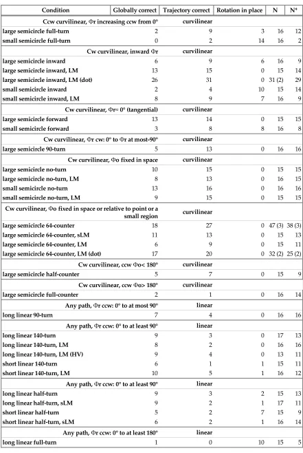
The experimental set-up has been described in detail in Bertin et al., 2000. We repeat here only the essentials. Optic flow stimuli consisted of dotscapes of white dots distributed (uniform, random; 4 pixel diameter; 4800 dots total) on a (50x50m) ground surface 1m below the virtual eye-level; the horizon was placed at 15m. The flow fields were gener-ated by simulating the movement of a virtual observer along the required manoeuvre, using Performer (Silicon Graph-ics). Each stimulus consisted of a 2s stationary period followed by 8s of simulated manoeuvre followed by another 2s stationary period. See figure 1a (insets A-C) for time-exposure impressions of stimuli (each with a landmark). Stimulus generation and display were under control of a Silicon Graphics Indigo2/Extreme workstation with a Virtual Research
VR4 head mounted display (HMD; FOV 48 horizontal, 36 vertical, 742x230 pixels, 60Hz refresh), and a Silicon Graph-ics O2 workstation with an NVision Datavisor LCD HMD (FOV 48 horizontal, 36 vertical, 640x480 pixels, 60Hz re-fresh). Presentation was binocular but monoscopic.
Subjects were required to reproduce their perception of the simulated manoeuvre after stimulus presentation. That is, they were to guide a model vehicle (a custom-made input device; inset E in figure 1a) through the manoeuvre they had just perceived, moving it over a graphics tablet. The device's instantaneous position (X,Y; resolution 22860x15240) and orientation ( o; resolution approx. 4 ) were read from the tablet using custom made software running on the Indigo, and saved to disk. During this reproduction, an overhead view of the tablet and the vehicle was presented in the HMD. A cursor showed the device's current position and orientation; previous positions remained visible as dots to in-dicate the travelled trajectory. Horizontal and vertical lines intersecting in the centre of the image were also shown as a frame of reference (inset D in figure 1a). Buttons on the device allowed the subjects to erase unsatisfactory reproduc-tions and accept (save) only those that best represented their percept.
Experimental procedure.
Subjects were instructed to concentrate on reproducing the perceived manoeuvre's geometry but to ignore its scale, making optimal use of the tablet's surface instead (resolution optimisation). After validating their response, they could ask for re-presentations of the same stimulus, until they were sure about the manoeuvre, and satisfied with the way they reproduced it. Similarly, when the experimenter noticed drawing/reproduction problems, or when subjects seemed unsure, they were asked to assess their result (from the image in the HMD), and to either erase and redraw it, or to view another presentation and repeat the reproduction. The experimenter took notes to allow for correct off-line interpretation of the reproductions.
Simulated manoeuvres.
The simulated manoeuvres are listed in Table 1, and shown in figures 1b through 1d. Triangular velocity profiles start-ing from zero velocity (angular and linear) and peakstart-ing at t=4s (half the stimulus duration) were used for comparison with earlier vestibular studies (Ivanenko et al., 1997a,b). The figures show the actual scale (in meters) of the simulated manoeuvres.
Landmarks, when present, were always fixed in the virtual environment, and visible during the whole stimulus pres-entation so that the additional information they provided was available the whole time. This constraint made it impos-sible to present all stimuli both with and without a landmark. The landmarks were constructed of dots identical to the dots making up the rest of the stimulus, except for their colour. Every landmark had a single red dot that was attached to the ground surface via a string of equally spaced blue dots (cf. figure 1a). Thus, a motion relative (in depth) to such a landmark could generate parallax (see inset B in figure 1a: the blue dots are smeared). Some landmarks moved through the observer's field of view, even though they were fixed in (3D) space: these are referred to as shifting land-marks (indicated with the suffix sLM). Subjects were required to keep the red dot fixated at all times. Thus, eye move-ments were made, that provided extra-retinal information. To test for a possible effect of parallax, stimuli with fixated
landmarks were presented5. In these stimuli, the red dot was stationary in the middle of screen (indicated with the suffix LM), while the simulated manoeuvre contained movement in depth relative to the landmark. Fixated landmarks were also used to test for the effect of the presence of a reference point alone in conditions without movement in depth rela-tive to the landmark, and in 2 conditions in which the red dot was placed directly on the ground surface. Note that the point to be fixated is always at eye-level6; when eye-movements are to be made, they are thus always horizontal (with
respect to the virtual environment), and the flow contains only radial and horizontal fronto-parallel components7 (cf.
Wann et al., 2000).
The simulated or reproduced manoeuvres are described at any given instant by a position in space, and three orienta-tions. Here, we are only concerned by the orientations: the observer's orientation in space ( o; independent of the trajec-tory), the orientation of the trajectory ( p: the angle in space of the tangent to the trajectory, i.e. the direction of move-ment) and the observer's orientation relative to the trajectory, r = o - p. Thus, we can distinguish two types of rota-tion: o (yaw) and p (the rotation of the trajectory). Angles are expressed in degrees, with negative values indicating clockwise rotation. Using these observables, the stimuli presented in this paper can be divided into 4 distinct classes, as shown in Table 1 and figure 1b-d. The control experiment served to shed additional light on the perception of manoeu-vres with yaw in the direction of, but less than, the path rotation. In this experiment, we presented semicircle no-turn,
! " #
$
% %
" $ & ' #
( "
semicircle 30-turn, semicircle 90-turn, semicircle 120-turn and semicircle forward, all with the small and the large ra-dius (not shown in figure 1).
Figure 1 about here.
At the beginning of each session, before the experiment proper, subjects were presented with 1) a simple forward translation and 2) a lateral translation ( o=90 : condition linear lateral). For these two stimuli, feedback was given to help the subjects arrive at the correct interpretation. This also served as a final check whether they completely under-stood the task, and to help them get used to the optic flow and its presentation in the HMD8.
) *+, % - .
% $ ( % (
. /0. % %
Table 1:
The presented stimulus conditions. The left column lists the condition name, the middle column a descrip-tion. The rightmost column lists the size of the simulated manoeuvre (L=length, R=radius, in meters); in which experiment it was presented (for experiment 3, this also indicates the type of landmark; s=shifting and f=fixated); and how the conditions are labelled in the figures. C= curvilinear; L= linear; labels are num-bered in order of increasing concordant yaw, with the lowest number corresponding to the condition with the largest counter yaw.
Condition Description Size [m ] 1 2 3 Fig
Stim uli with the observer's orientation (yaw ) fixed in space:
semicircle no-turn R=1.5, 5 - s C4
Stim uli with the observer's orientation fixed relative to the trajectory:
semicircle inward R=1.5, 5 - f C8
semicircle forward R=1.5, 5 - - C7
Stim uli with the observer's orientation changing in space and relative to the trajectory:
semicircle 90-turn R=1.5, 5 - - C5
semicircle full-turn R=1.5, 5 - - C9
linear 90-turn L=7.8 - - L5
linear 140-turn L=4.7, 7.8 - f L6
linear half-turn L=4.7, 7.8 - s L7
linear full-turn L=7.8 - - L8
rotation in place - - RIP
semicircle 64-counter R=5 - s,f C3
semicircle half-counter R=5 - - C2
semicircle full-counter R=5 - - C1
Semicircular trajectory with o=0
Semicircular trajectory, observer looking inward ("centripetal": r=-90
Semicircular trajectory with tangential orientation ( r=0
Semicircular trajectory with a quarter rotation ( o=90 starting at 0
Semicircular counterclockwise trajectory with a full rotation ( o=360 starting at 0
Linear translation with rotation o=90 (starting at 0
Linear translation with rotation o 140 (starting at 20
Linear translation with rotation o=180 (starting at 0
Linear translation with rotation o=360 (starting at 0
A o=-180 clockwise rotation.
Idem, with orientation changing in the direction opposite to the trajectory rotation: Semicircular clockwise trajectory with a 64
Data analysis.
Subjects could not see the tablet nor the vehicle they were manipulating (they could only see the result in the HMD); putting down or lifting the vehicle is difficult to do without introducing artefacts for this reason9. The reproduced
trajec-tories (traces) therefore often contained artefacts from the initial positioning of the vehicle, and small glitches due to the difficulty of controlling the vehicle. Some filtering was thus necessary to remove these initial and final artefacts; it was performed by one of the experimenter (RJVB, to maintain persistence). The artefacts were easily distinguishable from the actual, intended reproduction on simultaneous displays of the two spatial co-ordinates and of the orientation in time (X[t], Y[t] and o[t]) combined with an (X,Y, o) top-down view (cf. figure 1e), and using the notes taken during the experimental sessions.
The filtered traces were normalised to a fixed number of samples per trace for easier analysis, independent of the sub-stantial variation in the sampling rates in the raw data (the tablet only sent data when the vehicle moved and subjects' reproduction time and speed varied considerably). After initial smoothing, the data were therefore resampled to 20 equidistant points per trace. This was done with an interpolating algorithm that used cubic splines. Figure 1e shows an example of a filtered, raw (non-typical) reproduction, and its resampled version.
The resulting resampled reproductions were used to evaluate the subjects' performance. Performance was classified by visual examination of the individual responses using two criteria: overall correctness (globally correct) and the correctness of the trajectory (trajectory correct). The latter index gives a measure of how often subjects reproduced trajectories of the correct type (i.e. linear, "circular" or "in place"). The former index also takes reported yaw ( o) into account and requires stimulus-specific combinations of yaw and trajectory. For instance, for a lateral (or oblique) translation stimulus, a re-produced manoeuvre is globally correct when it is linear10 with the observer facing in the correct direction
(forward/backward) and at an perpendicular (or oblique) orientation to the path. This index gives a measure of how well the cardinal properties of a stimulus manoeuvre were perceived. Therefore, the expected illusory perceptions of ambiguous stimuli are also accepted as globally correct (e.g. a tangential curvilinear movement in response to condi-tion linear half-turn). We scored the number of globally correct and trajectory correct responses per condicondi-tion.
Our protocol only allowed us to analyse reproduced orientation ( ) and change in orientation (rotation; ). The three orientations and the two types of rotation that can be distinguished have been introduced above. Of these, we quanti-fied our results with p, o and the average orientation relative to the path < r>; cf. figure 1f and Bertin et al. (2000). For rotations in place, only o is defined. All the other conditions (manoeuvres) could be described by p, o and < r>11. This quantitative analysis was only applied to responses that were not rotations in place and that did not
con-tain changes in direction.
We tested for a landmark effects with ANOVA tests. We used relative error in o (yaw). For the rotation of the path, the p error was normalised to the presented o: this corrects for the attribution of yaw to path rotation that the sub-jects generally make.
We also analysed the responses with a figural distance measure, modified from Conditt et al. (1997). This measure quanti-fies the difference between stimulus and response, with zero indicating a perfect overlap. It is a measure that can be applied to all responses (whether or not a rotation in place), and that captures other aspects as well (e.g. three orthogo-nal linear segments can correspond to a 180° path rotation, while not being equal to a semicircle). Our measure (Df) consists of two independent components (Dfs and Dfa). A spatial figural distance (Dfs) was calculated as the average
! " ! # "$ !
of the pair-wise, squared distances between all points on the two trajectories (point 1 to point 1, point 2 to point 2, etc.12).
An angular figural distance (Dfa) was calculated as the average squared difference (maintaining the sign) between the orientations o in radians at the corresponding points (Dfa was normalised by (1+Dfs)/ to put Dfs and Dfa on a com-parable scale). For comparison over subjects and conditions, Dfs and Dfa were independently normalised to their re-spective maximal values over all responses being analysed. The combined figural distance was then calculated as the length of the vector spanned by the spatial and angular components: Dfs2 Dfa2. Prior to this analysis, the maximum overlap was determined between all stimulus/response pairs. This was done by shifting, scaling and rotating the re-sponse, under control of a Simplex downhill method.
Results
General observations.
Our results indicate that it is possible to reconstruct travelled paths from optic flow. However, almost all subjects indi-cated that this was a difficult task. Most indiindi-cated that they had experienced impressions of ego-motion (vection). When the stimulus simulated a relatively large amount of yaw relative to the simulated translation, subjects often reproduced a rotation in place. The presence of a landmark was perceived as helpful, but only in the cases where it was stationary in the field of view ("fixated"); otherwise it was considered a distraction.
Not all subjects systematically requested re-presentations. Very few subjects asked systematically for many (more than 3) re-presentations. In almost all cases, responses were consistent between re-presentations, with the final presenta-tion serving as a check, notably for the perceived direcpresenta-tion of rotapresenta-tion (that appeared to be easily forgotten). The re-sults we present hereafter are thus based on the final response only.
Response classification.
What kind of manoeuvres do subjects perceive in the task we ask them to do? Are their responses globally correct or at least trajectory correct? This response classification ("performance") of the subjects' reproductions is shown in figure 2, ex-pressed as percentages of the total number of responses. For completeness, the same data is listed Table 2, together with the number of samples per condition. The table also lists the number of rotation-in-place responses observed, and de-fines the globally correct and trajectory correct criteria for each stimulus.
Figure 2 & Table 2 about here.
Figure 2a shows the classification of the responses to the stimuli from experiment 1. When the observer's orientation is fixed in space (conditions linear lateral or oblique and semicircle no-turn), performance is generally good. Perform-ance decreases when the orientation is fixed only relative to the trajectory, or not at all. Good examples are conditions
semicircle inward and semicircle forward. The apparent difficulty of these stimuli is not caused by the simulated yaw in itself. Condition semicircle outward has exactly the same amount of yaw ( o) as the two aforementioned conditions, but is perceived more correctly (but the large radius version is often mistaken for a lateral translation, which leads to a lower globally correct score). Performance is generally better at the larger radius.
&' ( ) ( ! )
! & ! ! &
* ! ! !
) " + )
Figure 2b shows the classification for the responses to the conditions semicircle inward and semicircle no-turn with a landmark (darkly shaded; experiment 3) and without (lightly shaded; experiment 1). In most cases, there is a clear in-crease in performance when a landmark is present.
Quantitative analyses.
Subjects can accurately perceive the path-relative orientation when the orientation in space remains fixed (linear trajec-tories without yaw). On curvilinear paths, perception depends on the proportion of simulated rotation vs. translation, and on the simulated orientation relative to the path. Thus, perception was better for a large semicircle outward (but path rotation, p, was undershot) than for a semicircle forward, that was in turn better than perception for a semicircle
inward. When the radius was small, there were instead many rotation-in-place responses.
Influence of yaw (experiment 2).
Figures 3 shows the perceived yaw as a function of presented yaw ( o) and figure 4 shows the perception rotation of the path ( p) per condition. These observables are averaged over subjects, per condition, and include only those re-sponses that were not rotations in place and in which there was no change in direction of rotation (either o or p). This excludes responses that are clearly uncorrelated with the stimulus and for which p is undefined and/or ambigu-ous; Table 2 lists the number of responses retained in each case (the N* column).
Figures 3 & 4 about here.
Subjects appear to be capable to approximate the angle over which they are rotated, even during complex manoeuvres (figure 3). A small range effect occurs for the linear+yaw stimuli: overshoot for the smaller rotations, and undershoot for the large rotation ( o=360°). Difficulties in reproducing may partly account for this, as they may also (partly) for the large standard deviations in the more complex conditions. Does the good performance mean that on average subjects correctly perceive their simulated rotation, fully "specified" in the optic flow? Probably not, as shown by the cases in which rotations in place are (erroneously) reported ("RIP Responses" in the figure). It would appear that subjects incor-rectly perceive the simulated rotation when they are not capable of detecting the simulated displacement in the stimu-lus. Yaw is never perceived when the stimulus does not simulate any observer rotation (also cf. Bertin et al. 2000).
The perception of path rotation is shown in figure 4. Perception is close to veridical when orientation remains approxi-mately fixed in the environment ( o 0°), and when it is tangential to the trajectory. In the initial results, path rotation perception in condition semicircle 90-turn was not significantly different than in condition semicircle forward. This suggested that perception is close to correct when 0° o p . A control experiment (data shown in the figure) showed that path rotation is, or tends to be, undershot when o p , although the subjects who participated in both experiments did not respond differently in the control. Note that yaw perception is veridical in those conditions, ex-cept for condition semicircle 90-turn, and possibly condition semicircle 30-turn for which many subjects verbally re-ported the perception of no yaw (but they reproduced on average 30° of yaw).
When the orientation changes relative to the trajectory, such that o> p (this includes the linear+yaw conditions, where p=0°), subjects seem to assume that the detected rotation results (mostly) from a rotation of the trajectory. They respond in a similar manner when the simulated yaw is in the direction opposite to the direction in which the trajec-tory rotates. In this case, the number of reports of straight paths, or even paths curving in the wrong direction, increase with the presented o. This effect is so strong that in condition semicircle half-counter (a clockwise semicircle with a counterclockwise half-turn of the observer), the average perceived path is more or less a straight line. In condition
During these ambiguous stimuli, the perceived manoeuvre becomes increasingly incompatible with the simulated ma-noeuvre, possibly leading to corrections in the reproduction if this conflict is perceived. We split all responses in two equal parts, and compared the errors in the two halves (using ANOVAs) to test if such corrections occurred. We only found significant differences for the ambiguous stimuli. However, these differences were not systematic. Typically, the sign of the error changes, without a significant decrease or increase in absolute error. There is thus no support (neither in our current nor in our previously published data) for the hypothesis that the subjects correctly interpret a perceived mismatch between their initial percept and the simulated manoeuvre at some later time. Thus, it seems that most sub-jects adhere to the manoeuvre they perceive in the first moments of the stimulus presentation, regardless of whether a mismatch is perceived later on. There are subjects who correctly perceive these stimuli, however. These subjects often perceived "first a forward, tangential manoeuvre, then a lateral one, to finish with a backward curving manoeuvre".
Landmark effects (experiment 3).
Our results suggest that subjects are capable of detecting rotation (yaw) from the optic flow. However, when they must decide whether this rotation stems from a path rotating in space, or a change in orientation relative to a (linear) path, or both, almost all subjects choose the first possibility, apparently assuming a fixed orientation relative to curving path.
We presented a number of stimuli with and without a single, salient landmark that could provide additional visual in-formation, extra-retinal information (from eye-movements), or a combination of both. The significant effects of the presence of such a landmark are shown in figure 5 and concern mostly the linear+yaw responses since these were ana-lysed. There are significant improvements in yaw and path perception for the linear+yaw conditions, when a landmark is present (figures 5a and 5b). The improvement of the perception of the path is largest for the short translations, whereas the improvement in yaw is largest for the long translations. This means that the presence of a single landmark can improve the perception of the ego-motion component that is relatively weak: translation (the path) in case of a short linear+yaw manoeuvre, and rotation (yaw) in case of a long, otherwise identical manoeuvre.
Figures 5c and 5d compare the three different landmark conditions: no landmark, shifting through the field of view, and fixed at the centre of the HMD's field of view (fixated). The results suggest that the errors are smaller for a shifting landmark than for a fixated one. These results are significant again for o perception for the long translations, and for p for the short translations. The benefit of a landmark is also apparent from the normalised figural distance (ANOVA none vs. shifting vs. fixated; F(2,30)=4.58, p<0.0184; mostly due to the angular component), but for this measure, the effect of the fixated landmark is the largest. The number of erroneous RIP responses decrease when a landmark is present (ANOVA none vs. shifting vs. fixated; F(2,30)=4.81, p<0.0154).
There are too many RIP and invalid responses to perform a quantitative analysis of the landmark effect on yaw and path perception in the semicircular conditions. However, the angular figural distance (a measure of yaw perception) decreases in those conditions when a fixated landmark is present (ANOVA, F(1,14)=6.26; p<0.0254).
Discussion
ques-tion can thus also be reworded as: can human subjects integrate subsequent instantaneous percepques-tions of heading into a percept of a complex, 2D manoeuvre?
Our results show that subjects could perceive the qualitative nature of a simulated manoeuvre; correct directions, the correct form of trajectory and sometimes also the correct average orientation relative to the trajectory (< r>). How much of these qualitative aspects they perceived, and how well, depended on the complexity of the simulated manoeuvre. Human observers can thus indeed integrate their instantaneous perceptions of heading directions, at least to some ex-tent. This does of course not give any information about the distances travelled in these directions, since optic flow alone does not provide information on absolute linear ego-motion speed. An absolute judgement of the distance trav-elled can therefore not be made. But human observers are quite capable of making relative distance judgements from optic flow (Bremmer & Lappe, 1999; Bremmer et al. 1999). They can also estimate distances when the flow is generated by an accurate rendering of an environment they know well (Redlick, Jenkin et al., 2001). Finally, they can compare the radii of presented curvilinear manoeuvres (our unpublished results).
It is possible to quantitatively estimate rotation, i.e. turned angles, from the optic flow, at least in theory13. More
specifi-cally, it can be retrieved from the instantaneous flow field; no integration of information over time is necessary. Our re-sults suggest that subjects could indeed correctly detect the angle ( ) over which they were turned.
The reconstruction of the travelled trajectory was correct when the simulated trajectory was linear. The angle ( p) over which the trajectory rotates can be determined from the optic flow just as well as any other angle, again in theory. This should at least be so when the optic flow corresponds to a manoeuvre maintaining a fixed orientation relative to the travelled path. Then all rotation is caused by a rotation of the path. Subjects were indeed capable of correctly judging the rotation of the path when orientation was yoked to the path, but only when it was tangential to the trajectory. Percep-tion was much less veridical when the orientaPercep-tion was either inward (towards the centre of rotaPercep-tion, causing unreliable perception; perceived as rotations in place) or outward (away from the centre of rotation; perceived as rotations in place or as lateral translations when the radius was large). In general, when yaw need not be yoked to the path, correct perception requires that one can determine whether (and if so, how much) one-self rotates and whether the path (also) rotates.
A manoeuvre in which the observer moves with zero yaw (orientation fixed in space) along a circular trajectory is a spe-cial case: there is only path rotation. For these manoeuvres, perceived path rotation was also close to (but significantly different from) veridical (it was not good at all when subjects were physically displaced along such manoeuvres: cf. Ivanenko et al., 1997b). Perception was probably good because the rotation of the displacement vector was easily de-tectable in these flow fields; it was not masked by any other rotation. When yaw (in the same direction as the path ro-tation) increased, perception became less veridical (path rotation was undershot), until there was more than half as much yaw as path rotation.
The average reported path rotation was always less than the presented value for the stimuli discussed above, even if the difference was not always significant. This may be in line with the results from a recent study by van den Berg et al.
(2001) who found that subjects tend to undershoot the curvature of the simulated path. These authors measured head-ing and path-curvature perception from stimuli with less than 1s duration, not reconstruction as we did. Furthermore, curvature is inversely proportional to radius: a semicircle with a 10m radius will have half the curvature of a semicir-cle with a 5m radius, and yet they both have 180° path rotation. We did not measure scale (radius), so our results are
!
" # $
# %
&
not directly comparable to those of van den Berg et al. However, a number of our subjects reproduced smaller-than-180° circular arcs with a "flat" appearance (as if part of a big radius circle), and some described them as elliptical rather than circular. This may indeed correspond to an underestimation of the path's curvature.
We also presented stimuli in which there was yaw but no path rotation (linear trajectories), or more yaw than path rota-tion, or yaw in the direction opposite to the rotation of the path. Some of these stimuli are ambiguous, and give rise to illusory perception — that is they induce the perception of being on a trajectory other than the one actually simulated. A well known example is a "linear+yaw" stimulus that simulates a linear path travelled in combination with yaw (e.g. making a horizontal pursuit eye or head movement while walking straight forward). For such a stimulus, subjects are known to perceive curvilinear, tangential manoeuvres: they attribute the perceived rotation to a rotation of the path. We also found this behaviour in response to our version of this stimulus. We also found it when the path rotated (a semicircle), but there was more yaw (a full turn; some subjects then reported spiral manoeuvres) and when there was less yaw (120° or 90°; see above). Surprisingly, the attribution also occurred for the stimuli in which yaw was in the di-rection opposite to the path rotation. Thus, a semicircle could be perceived as a straight line, or as a curvilinear ma-noeuvre in the opposite direction, depending on the amount of yaw14. For condition semicircle 64-counter (64° counter
clockwise yaw and a clockwise semicircular path, no landmark), subjects on average perceived approximately 130° of path rotation.
Many authors have argued why this kind of illusion occurs. The primary reasons put forward are that 1) the optic flow resembles the flow corresponding to the illusory manoeuvre, and that 2) it simply does not provide enough informa-tion to choose between the alternative interpretainforma-tions. Thus, the simplest of the possibly matching manoeuvres is per-ceived. This is probably a sufficient explanation for short stimulus presentations, in which no big conflicts can occur between the illusory perceived manoeuvre (and its corresponding flowfield), and the manoeuvre specified by the optic flow. All of our linear+yaw stimuli evolved from a forward to a lateral manoeuvre, or beyond (i.e. backward), due to the amount of yaw simulated. Thus, there was an increasing incompatibility with the initially perceived, illusory manoeu-vre, that should create conflict. Yet, subjects in many cases reproduced manoeuvres that suggest that they more or less extrapolated the initially perceived manoeuvre. Comparison of the 1st and 2nd halves of their reproductions did not
re-veal any sign that they might have detected a conflict during the course of the stimulus, and adjusted their perception/response accordingly. Maybe not all subjects monitored the optic flow continuously for gradual changes in heading direction. They could instead have relied on qualitative changes in the simulated manoeuvre (or in the pre-sented optic flow) to update their perceived movement, extrapolating the initial percept as long as no such "events" oc-curred. Other subjects, generally experienced observers, did detect the qualitatively different phases, and arrived at (more) correct interpretations.
Can path perception from our longer, more complex stimuli that give rise to illusory perception also benefit from addi-tional, visual or extra-retinal information, as it can in shorter stimuli? To study this, we placed a single landmark in a number of our stimuli. This landmark provided additional extra-retinal information when it moved through the field of view; it provided additional visual information (parallax) when there was movement in depth relative to the land-mark. Even when it did not provide these two types of information, it could still serve as a reference for the movement of the other points (conditions semicircle inward).
In general, the subjects reported that the presence of a landmark facilitated the task, but only when it remained station-ary in the field of view. This was confirmed by the figural distance measure: the reproductions indeed resembled the actually presented manoeuvres more when a landmark was present than when it was absent.
For the linear+yaw conditions, perception of path rotation and yaw was more veridical when a landmark was present. This is in agreement with the study of Li and Warren (2000) who also found more veridical perception in shorter pres-entations of similar stimuli, but using many more landmarks. This result can also be compared to the results of van den Berg (1996) who finds that heading perception is "much more accurate" when subjects were asked to judge their
* + + %
heading relative to the perceived motion in depth of the fixation point that was stationary on the screen and corre-sponded to a fixed point in the virtual environment. In addition, we found that the perception of path rotation bene-fited more from the presence of a landmark when the simulated manoeuvre contained proportionally more yaw (that is, more in the short trajectory version than in the long version). Perception of yaw improved more due to a landmark when the simulated manoeuvre contained proportionally less yaw (that is, more in the long version than in the short version).
Perception also improved in some of curvilinear conditions. Much less responses to the conditions semicircle inward were excluded from analysis when the stimulus contained a landmark that only served as a reference for the move-ment of the other points, compared to when there was no landmark. There were also less erroneous rotation in place re-sponses when a landmark was present. In the majority of these conditions, however, there was little effect of adding a landmark, and sometimes even a negative effect. That means that either the additional information was of no use to the subject, or that the attention needed to interpret that information actually interfered with the ego-motion perception. Subject expectations may have played a role, for instance concerning what manoeuvre might occur in what environ-ment. But it is also likely that the structuring of an environment (the elements in addition to the "basic" elements, dots, that provide the optic flow) has to fulfil certain conditions that depend on the simulated manoeuvre, in order to be use-ful. The more complex the manoeuvre, the more additional elements (landmarks) that may be needed, for example. Adding more landmarks relaxes the big constraint faced with our single landmark, namely that at least one should be visible throughout the stimulus duration. This constraint was particularly big in the linear+yaw conditions. In these conditions, the shifting landmark moved across a large part of the field of view — in a zig-zag manner. Yet we have some tentative evidence for these conditions that the improvement of path rotation perception was bigger for a shift-ing landmark than for a non-shiftshift-ing landmark.
Two critical notes should be made about our response task. First, the good perception of yaw may in part be a result of an observational and/or response strategy. Our stimuli simulated manoeuvres with multiples of 90° and 180° of rota-tion. Subjects seemed to categorise in steps of at least 90°; estimating a large rotation that did not seem to be a full turn to be a half turn, or three quarters of a turn, and so forth. Similar observations were made in vestibular experiments by one of us (I. Israël). Sometimes subjects also indicated that they had little idea about the true amount of rotation, and their estimation was often considerably off when they erroneously perceived a rotation in place. But for stimuli simu-lating 64° yaw against 180° path-rotation in the other direction, the reported path rotation was around 130°. This was not significantly different from 180°-64°=116°, which suggests that the accuracy of rotation perception that we found was not solely due to a rough 90° categorisation. Second, the recorded reproductions that subjects made do not always exactly match how they verbally described them. For instance, in the semicircle 30-turn condition, many subjects de-clared having seen a semicircle no-turn manoeuvre, and yet the average reproduced yaw was approximately -32° — almost perfectly correct. It is impossible to tell whether the reproduction corresponded to the actual perception, and the verbal description was a categorisation; or whether the verbal description was closest to the actual percept, and the reproduction was just sloppy; or whether the truth was somewhere in the middle. This is indeed a weakness of our protocol, but similar, inherent problems are likely to exist in any psychophysical method, quantitative or qualitative.
References
Banks, M.S., Ehrlich, S.M., Backus, B.T., & Crowell, J.A. (1996). Estimating heading during real and simulated eye movements. Vision Res36, 431-443.
Bertin, R.J.V., Israël, I., & Lappe, M. (2000). Perception of two-dimensional, simulated ego-motion trajectories from optic flow. Vision Res40, 2951-2971.
Bremmer, F., Kubischik, M., Pekel, M., Lappe, M., & Hoffmann, K.P. (1999). Linear vestibular self-motion signals in monkey medial superior temporal area. Ann N Y Acad Sci871, 272-281.
Conditt, M.A., Gandolfo, F. & Mussa-Ivaldi, F.A. (1997). The motor system does not learn the dynamics of the arm by rote memorisation of past experience. J. Neurophysiol 78, 554-560.
Crowell, J.A. (1997). Testing the Perrone and Stone (1994) model of heading estimation. Vision Res37, 1653-1671. Crowell, J.A. & Banks, M.S. (1993). Perceiving heading with different retinal regions and types of optic flow. Percept
Psychophys53, 325-337.
Crowell, J.A., Banks, M.S., Shenoy, K.V., & Andersen, R.A. (1998). Visual self-motion perception during head turns.
Nature Neuroscience1, 732-737.
Cutting, J.E., Vishton, P.M., Flückiger, M., Baumberger, B., & Gerndt, J.D. (1997). Heading and path information from retinal flow in naturalistic environments. Percept Psychophys59, 426-441.
Gibson, J.J. (1950). The perception of the visual world. Boston: Houghton Mifflin.
Grigo, A. & Lappe, M. (1999). Dynamical use of different sources of information in heading judgments from retinal flow. J Opt Soc Am A Opt Image Sci Vis16, 2079-2091.
Hooge, I.T.C., Beintema, J.A., & van den Berg, A.V. (2000). Visual search of heading direction. Perception29, 10. Ivanenko, Y.P., Grasso, R., Israël, I., & Berthoz, A. (1997a). Spatial orientation in humans: perception of angular
whole-body displacements in two-dimensional trajectories. Experimental Brain Research 117, 419-427.
Ivanenko, Y.P., Grasso, R., Israël, I., & Berthoz, A. (1997b). The contribution of otoliths and semicircular canals to the perception of two-dimensional passive whole-body motion in humans. J Physiol (Lond)502 ( Pt 1), 223-233.
Kim,N.G. & Turvey,M.T. (1998). Visually perceiving heading on circular and elliptical paths. J Exp Psychol Hum Per-cept Perform 24, 1690-1704.
Lappe, M., Bremmer, F., & van den Berg, A.V. (1999). Perception of self-motion from visual flow [Review]. Trends in Gognitive Sciences3, 329-336.
Lee, D.N. (1974). Visual information during locomotion. In: R.B. MacLeod & H.L. Pick (Eds), Perception. Essays in honor of J.J. Gibson. (Ch. 14, pp. 250-267), Cornell University Press.
Lee, D.N. (1980). The optic flow field: the foundation of vision. Philos Trans R Soc Lond B Biol Sci290, 169-179.
Li, L. & Warren, W.H.Jr. (2000). Perception of heading during rotation: Sufficiency of dense motion parallax and refer-ence objects (in press). Vision Res
Redlick FP, Jenkin M, Harris LR (2001). Humans can use optic flow to estimate distance of travel. Vision Res. 41: 213-219.
Rieger, J.H. (1983). Information in optical flows induced by curved paths of observation. J Opt Soc Am73, 339-344. Royden, C.S. (1994). Analysis of misperceived observer motion during simulated eye rotations. Vision Res34,
3215-3222.
Royden, C.S., Banks, M.S., & Crowell, J.A. (1992). The perception of heading during eye movements [see comments].
Nature360, 583-585.
Royden, C.S., Crowell, J.A., & Banks, M.S. (1994). Estimating heading during eye movements. Vision Res34, 3197-3214. Royden, C.S. & Hildreth, E.C. (1996). Human heading judgments in the presence of moving objects. Percept Psychophys
58, 836-856.
Stone, L.S. & Perrone, J.A. (1997). Human heading estimation during visually simulated curvilinear motion. Vision Res 37, 573-590.
Turano, K.A. & Wang, X. (1994). Visual discrimination between a curved and straight path of self motion: effects of forward speed. Vision Res34, 107-114.
van den Berg, A.V. & Brenner, E. (1994a). Humans combine the optic flow with static depth cues for robust percep-tion of heading. Vision Res34, 2153-2167.
van den Berg, A.V. & Brenner, E. (1994b). Why two eyes are better than one for judgements of heading. Nature 371,
700-702.
van den Berg, A.V., Beintema, J.A. & Frens, M.A. (2001). Heading and path percepts from visual flow and eye pur-suit signals. Vision Res 41, 3467-3486
Wann, J.P., Swapp, D., & Rushton, S.K. (2000). Heading perception and the allocation of attention. Vision Research40,
2533-2543.
Warren, W.H.Jr. & Saunders, J.A. (1995). Perceiving heading in the presence of moving objects. Perception24, 315-331. Warren, W.H.Jr, Blackwell, A.W., Kurtz, K.J., Hatsopoulos, N.G., & Kalish, M.L. (1991a). On the sufficiency of the
ve-locity field for perception of heading. Biol Cybern65, 311-320.
Warren, W.H.Jr. & Hannon, D.J. (1990). Eye movements and optical flow. J Opt Soc Am [A]7, 160-169.
Warren, W.H.Jr., Mestre, D.R., Blackwell, A.W., & Morris, M.W. (1991b). Perception of circular heading from optical flow. J Exp Psychol Hum Percept Perform17, 28-43.
Acknowledgements
Tables:
Legend to Table 2
Condition Globally correct Trajectory correct Rotation in place N N*
Ccw curvilinear, r increasing ccw from 0° curvilinear
large semicircle full-turn 2 9 3 16 12
small semicircle full-turn 0 2 14 16 2
Cw curvilinear, inward r curvilinear
large semicircle inward 6 9 6 16 9
large semicircle inward, LM 13 15 0 15 14
large semicircle inward, LM (dot) 26 31 0 31 (2) 29
small semicircle inward 2 4 10 15 14
small semicircle inward, LM 8 9 7 16 9
Cw curvilinear, r 0° (tangential) curvilinear
large semicircle forward 13 14 0 15 15
small semicircle forward 3 8 8 16 8
Cw curvilinear, r cw: 0° to r at most-90° curvilinear
large semicircle 90-turn 5 13 0 16 16
Cw curvilinear, o fixed in space curvilinear
large semicircle no-turn 10 15 0 15 15
large semicircle no-turn, LM 8 13 0 16 15
small semicircle no-turn 13 16 0 16 16
small semicircle no-turn, LM 9 15 0 15 15
Cw curvilinear, o fixed in space or relative to point or a
small region curvilinear
large semicircle 64-counter 18 27 0 47 (3) 38 (3)
large semicircle 64-counter, sLM 11 13 0 15 13
large semicircle 64-counter, LM 6 9 0 15 11
large semicircle 64-counter, LM (dot) 17 20 0 32 (2) 25 (2)
Cw curvilinear, ccw o< 180° curvilinear
large semicircle half-counter 5 7 0 15 9
Cw curvilinear, ccw o> 180° curvilinear
large semicircle full-counter 2 1 0 16 14
Any path, r ccw: 0° to at most 90° linear
long linear 90-turn 7 4 0 16 16
Any path, r ccw: 0° to at least 90° linear
long linear 140-turn 9 3 0 17 13
long linear 140-turn, LM 8 2 0 16 16
long linear 140-turn, LM (HV) 9 4 0 13 11
short linear 140-turn 6 1 1 15 11
short linear 140-turn, LM 10 5 1 16 12
Any path, r ccw: 0° to at least 90° linear
long linear half-turn 9 3 2 15 13
long linear half-turn, sLM 9 2 1 17 11
short linear half-turn 5 2 7 15 9
short linear half-turn, sLM 6 2 1 16 14
Any path, r ccw: 0° to at least 180° linear
long linear full-turn 1 0 10 15 5
Legends to the figures:
Legend to figure 1:
1a: Information displays in the head mounted display: impressions of the optic flow stimuli and the feedback during reproduction. In the experimental conditions, only single dots were seen to be moving, with a slightly higher den-sity and otherwise identical geometry and field of view. See Table 1 for detailed descriptions of the stimuli. A): con-dition linear half-turn with a shifting landmark (after 1.87s); B) concon-dition semicircle 64-counter with a fixated landmark (after 2.4s); C) condition semicircle no-turn with a shifting landmark (after 4.68s). D) an example of the reproduction feedback the subjects saw in the HMD: here, the input device was guided through a tangential, cur-vilinear manoeuvre (from left to right). E) an exploded view of the "vehicle", the input device manipulated by the subjects.
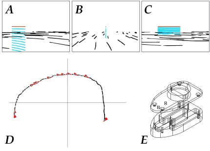
1b: Top-down view of the stimuli; experiment 1. Each curve represents a trajectory (X,Y), the arrows point in the di-rection of the observer's orientation ( o) at the indicated locations. The figure shows only the large conditions, from left to right, top to bottom:
(left): L1: linear lateral, L2: linear oblique 30 , L3: linear oblique 120 ; L4: linear oblique 135 .
(middle): C6: semicircle outward ( r=90 ); C7: semicircle forward ( r=0 ); RIP: the rotation in place; C8:
semicir-cle inward ( r=-90 ).
(right): C4: semicircle no-turn; C9: semicircle full-turn; L7: linear half-turn.
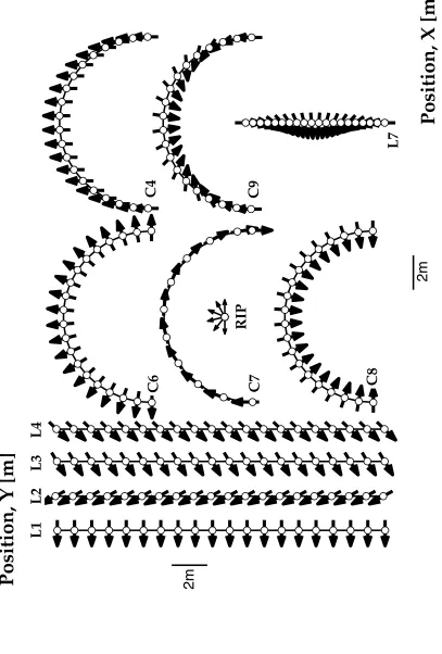
1c: Top-down view of the stimuli; experiment 2. Presentation as described for figure1b. For simplicity, those stimuli from set A that will directly be compared to stimuli from set B are also shown, whereas those that will be com-pared to stimuli from set C are shown in figure 1d. C1: semicircle full-counter; C2: semicircle half-counter; C4:
semicircle no-turn; C5: semicircle 90-turn; C7: semicircle forward; C9 semicircle full-turn; L5: linear 90-turn; L7:
linear half-turn; L8: linear full-turn.
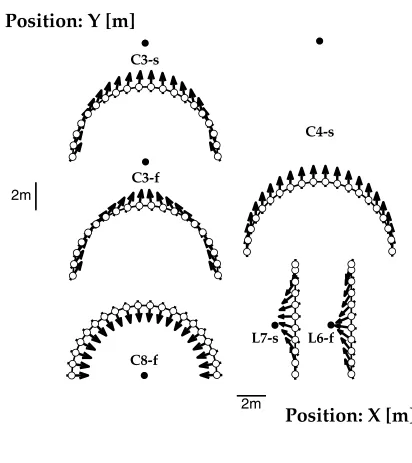
1d: Top-down view of the stimuli; experiment 3. Presentation as described for figure 1b; landmarks are shown as large filled dots (labelled with the same label as the corresponding manoeuvre). All stimuli were presented at least once with and once without the landmark at the indicated position. No distinction is made in this figure be-tween the different types of landmark. C3-s: semicircle 64-counter, sLM; C3-f: semicircle 64-counter, LM; C4-s:
semicircle no-turn, LM; C8-f: semicircle inward, LM; L6-s: linear half-turn, LM; L6-f: linear 140-turn, LM. Note the small differences between C3-s and C3-f, and L7-s and L6-f.
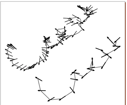
1e: Example of a raw reproduction (after filtering of initial artefacts; left-upper trace) and the same response resam-pled to 20 approximately equidistant points (lower-right trace). Reproductions are dimensionless, hence no scale is shown.
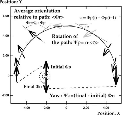
1f: Explanation of the indices used in the quantitative analyses. p, the average rotation of the path is calculated from the average difference between the tangents to the trajectory in 2 consecutive (resampled) points, multiplied by the number of segments per curve (19). The total yaw o is calculated by (non circular) summation over o, minus the initial orientation; thus, 2 full observer turns give o=720 . The average orientation relative to the path, < r>, is calculated as the average difference between o and p in the 20 resampled points. All these measures are ex-pressed in degrees and averaged over subjects. In this example (semicircle half-counter), o=180 , p=-180 and < r>=179.7 109.8 .
Legend to figure 2:
Response classifications (performance): globally correct responses (upward bars) and responses with the correct type of trajectory (downward bars), expressed as a percentage of the number of observations. Transparent downward bars with dashed outline show the percentage of responses that could be quantitatively analysed.
reported on in the present paper. Condition semicircle no-turn is labelled smcirc. fixed in the figures. See the text for the remaining details.
2b: Performance for selected semicircular stimuli from experiment 1 (lightly shaded) and 3 (dark shaded). The with-landmark (exp. 3) conditions are labelled with only their with-landmark type; the manoeuvre is that of the non-land-mark (exp. 1) condition to their immediate left. The benefits of the presence of a single landnon-land-mark are clearly visible — to the exception of the conditions large no-turn (smcirc. fixed), but especially for condition large inward.
Legend to figure 3:
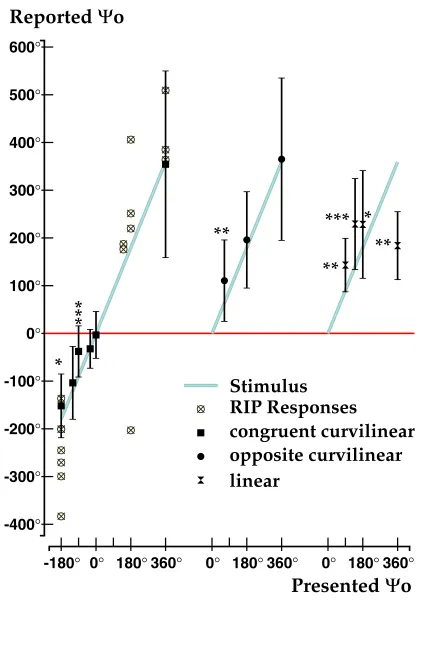
o (yaw) responses for all conditions from experiments 1 and 2 with o 0° and initial o=0° against the presented o. The leftmost collection also shows the responses to the curvilinear stimuli with congruent o (including data from the control experiment). The middle collection shows the responses to the curvilinear stimuli with o oppo-site to p, and the rightmost collection the responses to the linear+yaw stimuli. Ideally, the responses should all fall on the shaded lines. Points with errorbars (standard deviation in the mean) each represent the average of all responses to one particular manoeuvre, lumped over all sizes at which that manoeuvre was presented. The left-most collection also shows the o for all cases were the subjects reported rotations in place. These are not lumped over size, and, for clarity, the standard deviations are not shown. Asterisks indicate significant deviation from the expected values, determined by Student's t-tests using mean and average standard deviation; * p< 0.05, ** p< 0.005, *** p< 0.001 . The counter-yaw conditions are labelled opp(osite) in the figures. The number of retained samples per observation is listed in the N* column, Table 2.
Legend to figure 4
Rotation of the path ( p) responses (light shaded bars) for all conditions with initial orientation o 0°, averaged over all sizes in which each condition was presented. Dark shaded bars show the expected (i.e. stimulus) values. The conditions are ordered according to decreasing counter-clockwise rotation/increasing clockwise rotation. The re-sponse value for condition semicircle 64-counter is the mean over all rere-sponses to the 3 presentations of this stimulus (without landmark). Condition semicircle 120-turn (C11; n=13) and semicircle 30-turn (C10; n=14) were presented in the control experiment. The other results from this experiment are incorporated in the averages shown for the corresponding conditions: semicircle no-turn (n=29), semicircle 90-turn (n=32) and semicircle
for-ward (n=31). Errorbars show standard deviation of the mean. Asterisks indicate significant differences from the ex-pected values, determined by Student's t-tests using mean and average standard deviation; * p< 0.05, ** p< 0.005, *** p< 0.001 . The number of retained samples per observation is listed in the N* column, Table 2.
Legend to figure 5:
Effects of landmark presence on the perception of yaw ( o) and path rotation ( p). The graphs show the results from ANOVAs (StatSoft Statistica 5.1E) on the difference with the expected values. For o, relative error is shown. For p, we show the error relative to the presented o (yaw-relative error), because of the observed attribution of path-relative yaw to path-rotation.
5a: Plot of means for landmark presence on the perception of o in (long and short) conditions linear 14-turn; linear
14-turn, LM; linear half-turn; linear half-turn, sLM. There is a significant increase in performance when a land-mark is present for the long (large) translations.
5b: Plot of means for landmark presence on the perception of p in the same conditions. There is a significant increase in performance when a single (shifting or fixated) landmark is present, due mostly to the effect on the perception of the small (short trajectory) stimuli (landmark/size interaction; p<0.03).
5c: Plot of means, influence of landmark presence and type on o perception for all conditions linear 140-turn and the conditions linear half-turn. The benefit of landmark presence is significant for the large translations; especially for a shifting landmark (p<0.035 for the large translations; marginally significant over all responses).
A
B
C
D
E
2m
2m
P
o
si
ti
o
n
,
Y
[
m
]
P
o
si
ti
o
n
,
X
[
m
]
R
IP
L
7
C
9
C
4
C
8
C
7
C
6
L
1
L
3
L
4
L
2
2m
2m
P
o
si
ti
o
n
:
Y
[
m
]
P
o
si
ti
o
n
:
X
[
m
]
L
8
L
5
C
1
C
2
C
5
L
7
C
9
C
4
C
7
Figure 1d
2m
Position: Y [m]
Position: X [m]
L6-f
L7-s
C4-s
C8-f
C3-f
C3-s
-2.00 0 2.00 4.00 6.00
-4.00 -2.00 0 2.00 4.00
Position: Y
Position: X
Yaw :
Ψο
=(final - initial)
Φ
o
Rotation of
the path:
Ψ
p= n
⋅
<
ϕ
>
Average orientation
relative to path: <
Φ
r>
Φ
r=
Φ
o-
Φ
p
ϕ
Initial
Φ
o
Final
Φ
o
ϕ = Φp(i) − Φp(i−1)
D o c: cm b 3 p u b _ 1 d 3 .s d w — P ag e: 2 7 /3 1 — D at e: T u e 1 F e b ru a ry 2 0 0 0 ( A g e: 0 0 :5 5) — L as t p rin te d : 2 0 0 2 0 3 0 8 2 1 :1 5
100%
80%
60%
40%
20%
0%
20%
40%
60%
80%
100%
RIP L1 L2 L3 L4 C4 c4 C6 c6 C7 c7 C8 c8 C9 c9 L7 l7
Condition
Globally correct responses
Trajectory correct responses
Dashed bars: quantitatively analysed responses
RIP: rot. in place
L1: lin. lateral
L2: lin. oblq. 30
°
L3: lin. oblq. 120
°
L4: lin. oblq. 135
°
C4: l. smcirc. fixed
c4: s. smcirc. fixed
C6: l. smcirc. outw.
c6: s. smcirc. outw.
C7: l. smcirc. forw.
c7: s. smcirc. forw.
C8: l. smcirc. inw.
c8: s. smcirc. inw.
C9: l. smcirc. full
c9: s. smcirc. full
L7: l. lin. 180
°
yaw
l7: s. lin. 180
°
yaw
u
re
2
a
D o c: cm b 3 p u b _ 1 d 3 .s d w — P ag e: 2 8 /3 1 — D at e: T u e 1 F e b ru a ry 2 0 0 0 ( A g e: 0 0 :5 5) — L as t p rin te d : 2 0 0 2 0 3 0 8 2 1 :1 5
100%
80%
60%
40%
20%
0%
20%
40%
60%
80%
100%
c8
c8-f
C8
C8-f
C8-fd C8-Fd
c4
c4-s
C4
C4-s
Semicircle conditions
Condition
C8: l. smcirc. inw.
c8: s. smcirc. inw.
C4: l. smcirc. fixed
c4: s. smcirc. fixed
Landmarks types:
s: shifting
f: fixated, yaw
F: fixated, yaw+tilt
d: dot only
Globally correct responses
Trajectory correct responses Dashed bars: quantitatively analysed responses
u
re
2
b
-400
°
-300
°
-200
°
-100°
0
°
100
°
200
°
300
°
400
°
500
°
600
°
-180
°
0
°
180
°
360
°
0
°
180
°
360
°
0
°
180
°
360
°
Reported
Ψ
o
Presented
Ψ
o
Stimulus
RIP Responses
congruent curvilinear
opposite curvilinear
linear
**
*** *
**
**
***
*
-300°
-200°
-100°
0
°
100°
200
°
300°
400°
500°
600°
C7 C11 C5 C10 C4 C3 C2 C1 C9 L5 L6 L7 L8
Ψ
p
Condition
C7 : l. smcirc. forw.
C11: l. smcirc. 120° yaw
C5 : l. smcirc. 90
°
yaw
C10: l. smcirc. 30° yaw
C4 : l. smcirc. fixed
C3 : l. smcirc. 64° opp
C2 : l. smcirc. 180
°
opp
C1 : l. smcirc. 360
°
opp
C9 : l. smcirc. 360° yaw
L5 : l. lin. 90° yaw
L6 : l. lin. 140° yaw
L7 : l. lin. 180
°
yaw
L8 : l. lin. 360
°
yaw
**
**
*
*
**
***
***
***
***
Stimulus
Response
Linear+yaw; Path perception (yaw-relative error) -0.2 0.0 0.2 0.4 0.6 0.8 1.0 1.2 1.4 none present
Landmark Main Effect; F(1,4)=12.28; p< 0.0248
Landmark/Size interaction F(1,4)=12.17; p< 0.0252
Linear+yaw; Yaw perception (relative error)
-0.2 -0.1 0.0 0.1 0.2 0.3 0.4 0.5 0.6 0.7
Long: F(1,7)=21.69; p< 0.0023
Ψo[°] Linear+yaw; Yaw perception (relative error)
-0.2 -0.1 0.0 0.1 0.2 0.3 0.4 0.5 0.6
Long, landmark main effect F(2,18)=4.06; p< 0.0349 Landmark main effect, none vs. shifting
F(1,5)=4.83; p< 0.079
0.0 0.2 0.4 0.6 0.8 1.0 1.2 1.4
none shifting fixated
None vs. shifting: F(1,10)=5.20; p< 0.0458
None vs. present: p< 0.053
Linear+yaw; Path perception (yaw-relative error)
Landmark Main Effect; F(2,14)=4.21; p< 0.0370
Ψp[°]