An EPQ Inventory Model For Deteriorating Items With Weibull Deterioration Under Stock Dependent Demand

232

An EPQ Inventory Model For Deteriorating Items

With Weibull Deterioration Under Stock

Dependent Demand

N. K. Kaliraman, R. Raj, S. Chandra, H. Chaudhry

Abstract: This paper develops an economic production quantity inventory model for deteriorating items; the rate of deterioration is Weibull distribution deterioration with two parameters. The rate of demand is stock dependent. Shortages are not allowed. The aim of this study is to find the optimal solution for minimizing the total inventory costs. To optimize the model a numerical illustration has been carried out and a sensitivity analysis occurred to study the result of parameters on assessment variables and the entire cost of this model.

Keywords: Deteriorating Items, EPQ Model, Stock Dependent Demand, Weibull Deterioration

————————————————————

1. Introduction:

An economic production quantity model determines the quantity a company or a retailer must order to minimize the total inventory cost by balancing the inventory holding cost and fixed ordering cost. An economic production quantity model is an extension of economic order quantity model. In the usual inventory system, it was considered that the buyer pays to vendor as soon as he receives the goods. Inventory is frequently replenished from time to time at guaranteed production rate which is rarely infinite. Goods deteriorate and their values decreases with time. Electronic products may become obsolete as technology changes; fashion trends depreciate the value of cloths over time; batteries die out as they old. The outcome of time is even more serious for consumable goods such as foodstuff and drugs. The shortages are not allowed. All demands are satisfied immediately. In recent research, Covert and Philip [1] presented an inventory model where the time to deterioration is described with two parameter Weibull distribution. Ghosh and Chaudhuri [2] presented an inventory model for Weibull deteriorating items with two parameters, shortages are allowed and demand rate is quadratic.

They presented infinite series representation at initial stage and total relevant cost equation. Sanni [3] proposed an inventory model for Weibull deteriorating items with three parameters, shortages are allowed and demand rate is quadratic. He presented an explicit equation at initial stage and total relevant cost by tailor series approximation. Goyal and Giri [4] presented a review on inventory model with deteriorating items. Most deteriorating inventory model consider constant rate of deterioration. Berrotoni[5] presented that Weibull distribution deterioration can be applied for leakage failure of dry batteries and life expectancy of ethical drugs. The rate of deterioration increased with age and the rate of failure was high in both cases. Wu and Lee [6]; Mondal et al. [7]; Chen and Lin [8]; Ghosh and Chaudhuri [9]; Mahapatra and Maiti [10] extended many inventory models with deteriorating items which follows Weibull distribution deterioration. Deb and Chaudhuri [11] extended he inventory model with shortages to the inventory model of Donaldson [12]. Dave and Patel [13] considered linearly trended demand and no shortages in inventory models with deteriorating items. Manna and Chaudhauri [14] developed an inventory model for deteriorating items with unit production cost, shortages and time dependent deterioration rate. They assumed linear trend in demand and considered that time dependent demand rate proportional to finite production rate and time proportional to deterioration rate. A deterministic inventory model for deteriorating items with finite production rate, price dependent demand rate and varying deterioration rate with time value of money over a fixed time horizon developed by wee and Law [15,16]. The main purpose of this paper is to show that there exist a unique optimal cycle time to minimize the total inventory cost per unit time. A numerical example is presented to show the result of the proposed model.

2. Assumptions:

The following assumptions are used to develop mathematical model:

1. The Inventory system consider single item. 2. The inventory level defined by

I t

 

at time t.

Where

 

 

1

1 0, 0

0, a

b

I t t t

I t t t T

   



 _{  }

  __________________________

 Naresh Kumar Kaliraman is currently pursuing Ph D in Mathematical Sciences in Banasthali University, Rajasthan-304022, India, PH-09891008069,

E-mail: [email protected]

 Co-Author: Ritu Raj is currently pursuing Ph D in Mathematical Sciences in Banasthali University, Rajasthan-304022, India, PH-09711717006,

E-mail: [email protected]

 Co-Author: Dr Shalini Chandra is currently working as an Associate Professor in Mathematical Sciences in Banasthali University, Rajasthan-304022, India, PH-07891434849, E-mail: [email protected]

3. The demand rate

D t

 

is defined as

 

 

D t

 

R

aI t

, where

R



0

,

a



0

are constants and

I t

 

is retailer’s stock level. 4. The lead time is zero.

5. Shortages are not allowed. 6. Cycle horizon is infinite.

7. The rate of deterioration is time dependent, which is two parameters weibull distribution deterioration denoted by

 



t

1, where

0

 



1,





1

and

t



0

.

A value of

t



1

defines that the failure rate decreases with time. This happens if defective items fails at earlier stage and the failure rate decreases with time. A value of

t



1

defines that the failure rate is constant with time. A value of

1

t



defines that the failure rate increases with time.

3. Notations:

The following notations are used to develop mathematical model:

P

: Annual production rate.

A

: Theordering cost per unit.

r

: Raw material cost per unit.

l

: Labor cost.

w

: The wear and tear cost.

e

: Cost due to environment protection.

c

h

: The stock holding cost per year.

s

h

: The setup cost.

T

: Length of time in years.

T

: Optimum cycle length.

TC

: Total inventory cost

K

: Production cost per unit, denoted by

l

K

r

wP e P

P

  



, where

P

is production rate

per year,

r

is the raw material cost per unit,

l

is the labor cost,

w

is the wear and tear cost,

e

is the environmental cost.

4. Mathematical Model:

At the start of the cycle, the constant production starts at

0

t



and continues up to

t



t

₁. At this stage the inventory level reaches its maximum level and then production is stops. The inventory depletes to zero due to demand and deterioration at the end of the production cycle at

t



T

. The effect of demand, production and deterioration is applicable during the time interval

 

0,

t

₁ . The producer is assured to produce more items as demand increases. From the nature of solution of model, it is necessary that





1

,



and

t

are positive. Therefore, the inventory is described by the system of differential equations:

 

_{ }

_{ }

1

, 0

a

a

dI t

I t P D t t t

dt       (4.1)

Where

 

 

1

,

a

D t

 

R

aI

t

 



t

 , with boundary condition

 

0

0

a

I



The combined effect of demand and deterioration is applicable during the interval

 

t T

₁

,

. Therefore, the inventory is described by the system of differential equations:

 

_{ }

_{ }

1

,

b

b

dI t

I t D t t t T

dt      _(4.2)

 

With boundary condition

I T

b



0

The solution of equation (4.1) is

 





1

1 t

a

t

I t e  P R t



 

 

   

 _  _  _



 

  _(4.3)

The solution of equation (4.2) is

 







1 1



1 t

b

I t e R T t  T t



    

 _    _



  _(4.4)

Consider continuity

I t

 

at t



t

₁, it follows that













1

1

1 1

1

1 1 1

1

1

1

t

t

e P R

T t

t

t e R

T t











 











 

 



  

  _{ }

 

 _  _{ } 

  _{  }

 

 



 



1 1

1 1 1 1

R

t t T T

P

 

234



2



1

1 1 2

, 1 R T T P t









      (4.5)

Based on the assumption, the total relevant cost TC includes the following elements:

1. Ordering cost per year

A

T



2. Stock holding cost per year during the interval

 

0,

T

is:

  1    

1 0 0 t T T c c a b t h h

I t dt I t dt I t dt

T T          











2 4 3 2 2 2 2 2 2 1 1

8 2 3

3 2

2 2 2 2

3 3 3 3

1 2

c

R R R R

T T

P P

R PR R

T R T

P h

T _{P R R P}

T T R T T P           _  _  _                _{    }         _ _       _{ }    _   _         _{ }     

3. Cost of deterioration per year during the interval

 

0,

T

is .





2 4 3 2 2 2 2 2 2 1 1

8 2 3

3 2

2 2 2 2

3 3 3 3

1 2

R R R R

T T

P P

R PR R

T R T

P r

T P R R P

T T R T T P           _  _  _    _ _ _ _    _   _ _      _ _       _{ }   _   _         _{ }     

4. Production cost per year

KPt

1

T



5. Setup cost per year

h

s

T



The total relevant cost of the retailer is given by TC (T) = ordering cost + holding cost + cost of deterioration+ production cost + setup cost

 









1 2 4 3 2 2 2 2 2 2 1 1

8 2 3

3 1

2

2 2 2 2

3 3 3 3

1 2

s c

A KPt h h r

R R R R

T T

P P

R PR R

T R T

TC T P

T

P R R P

T T R T T P                     _  _  _          _{   }        _   _ _  _        _{     }    _{ }      _   _              _{   }    

 





4 3 2

1 1 1 1 1

2 2

1 1 1 1 1 1

1 AT B T C T D T E

TC T

T FT G T H J T L T M

      

 



     

  (4.6)

Where 2





1 1

8 c

R h r R

A P      _  _   ,





1 1 2 3 c

R h r R B

P

   

 _  _

 

,

_

_

2

1

3 2

c

R PR

C h r

P      _{ }   ,

_

_

1 c R

D h r R

     _  _   ,





1 2 2 3 c s

P h r

KP

E A h

       ,





1 2 3 c

R h r

F P   ,   1 2 3 c

R h r

G

P





 , 1  2

2 3

c

h r P K P H      , 2 1

J





R

,

L

₁



2



R

,

M

₁



P

Solution: All parameters are defined on

T



0

and total

relevant cost is continuous and well defined.













3 2

1 1 1 1 1 1

2

1 1 1

2 1 1

1 1 1 ₂

1 1 1 4 3 2

1 1 1 1 1

2 2 2

1 1 1 1 1 1

4 3 2 2

1

2 2 1

A T B T C T D F T G TC

J T L T M T T

J T L F T G T H

J T L T M A T B T C T D T E

T F T G T H J T L T M

   _{    }     _{    }    _{  }    _{ }                        (4.7)





















2

1 1 1

2

1 1 1 1 1 1 2 1 1

2

1 1 1 2

2 1 1 1

1 1 3

2 2

1 1 1

3 2

1 1 1 1 1 1

2

1 1 1 2

2 1 1

1 1 1 ₂

1 1

12 6 2

2 2

2 1

4 3 2 2

2

2 2 A T B T C

F J T L T M F T G J T L

F T G T H TC

J T L T M

T T

J M

J T L T M

A T B T C T D F T G J T L T M

T

J T L F T G T H

J T L T

              _   _{  }   _{  }                _{ }                    





1 4 3 2

1 1 1 1 1

3 2 2

1 1 1 1 1 1

2

M A T B T C T D T E

T F T G T H J T L T M

                                    (4.8)

Main objective to minimize the total relevant cost TC, the necessary condition to minimize the total relevant cost is

0

TC

T



_



, we get

 

 

4 3 2

1 1 1 1

4 3

1 1 1 1 1 1 1 1 2

1 1 1 1 1 1 2

1 1 1

3 2

4 3 2

2 2

0 2

A T B T C T E

F J T F L G J T H L T F M G L T H M

J T L T M

Using the software Mathematica, we can calculate the optimal value of T by equation (4.9) and the optimal value TC (T) of the total relevant cost is determined by equation (4.6). The optimal value of T satisfy the sufficient condition for minimizing total relevant cost TC (T) is

2

2 0

TC T

 _

 _(4.10)

The sufficient condition is satisfied.

5. Numerical Examples:

Example1: Let us consider

P



100

units per year,

500

R



units per year,

A



Rs

2000

per order,

15

c

h



Rs

per unit,

h

_s



Rs

1500

per unit,

r



Rs

4

per unit,

K



Rs

7.1

per unit,





0.9

,





1

,

l



Rs

200

,

0.0005

w



Rs

,

e



Rs

0.1

, then the optimal value of T is

0.370

T



and

TC



14753.25

Example 2: Let us consider

P



100

units per year,

500

R



units per year,

A



Rs

2500

per order,

15

c

h



Rs

per unit,

h

_s



Rs

1875

per unit,

r



Rs

4

per unit,

K



Rs

7.9

per unit,





0.9

,





1

,

l



Rs

250

,

0.0006

w



Rs

,

e



Rs

0.13

, then the optimal value of T is

T



0.395

and

TC



17250.5

6. Sensitivity Analysis:

To know, how the optimal solution is affected by the parameters, we derive the sensitivity analysis for some parameters. From the given numerical example, we derive the optimum solution. The finest values of some parameters are increases or decreases by

25%, 25%



and

50%, 50%



. We derive the value of

K

with the help of increased or decreased values of

l

,

w

and

e

. After that, we derive the value of

T

and

TC

with the help of increased or decreased values of

A

,

h

_sand

K

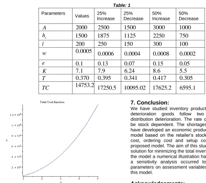
. The result of total relevant cost is existing in the following table 1.

Table: 1

Parameters

Values 25% Increase

25% Decrease

50% Increase

50% Decrease

A

2000

2500

1500

3000

1000

s

h

1500

1875

1125

2250

750

l

200

250

150

300

100

w

0.0005

0.0006

0.0004

0.0008

0.0002

e

_0.1

_0.13

_0.07

_0.15

_0.05

K

7.1

7.9

6.24

8.6

5.5

T

0.370

0.395

0.341

0.417

0.305

TC

14753.25

17250.5

10095.02

17625.2

6595.1

Fig. 2.Graphical representation of total relevant cost function without shortage.

7. Conclusion:

We have studied inventory production system where the deterioration goods follow two parameters Weibull distribution deterioration. The rate of demand assumed to be stock dependent. The shortages are not allowed. We have developed an economic production quantity inventory model based on the retailer’s stock level. The production cost, ordering cost and setup cost much affected the proposed model. The aim of this study is to find the optimal solution for minimizing the total inventory costs. To optimize the model a numerical illustration has been carried out and a sensitivity analysis occurred to study the result of parameters on assessment variables and the entire cost of this model.

Acknowledgements:

236

References:

[1] R. P. Covert, G. C. Philip, “An EOQ model for items with Weibull distribution deterioration,” AIIE Trans. 5, 323-326,1973.

[2] S. K. Ghosh, K. S. Chaudhuri, “An order-level inventory model for a deteriorating item with Weibull distribution deterioration, time-quadratic demand and shortages,” Adv. Model. Optim. 6(1), 21-35,2004.

[3] S. S. Sanni, “An economic order quantity inventory model with time dependent Weibull deterioration and trended demand,” M. Sc. Thesis, University of Nigeria, 2012.

[4] S. K. Goyal, B. C. Giri, “Recent trends in modeling of deteriorating inventory,” European Journal of Operational Research, 134, 1-16,2001.

[5] J. N. Berrotoni, “Practical applications of Weibull distribution,” ASQC Tech. Conf. Trans., 303-323,1962.

[6] J. W. Wu, W. C. Lee, “An EOQ inventory model for items with Weibull distributed deterioration, shortages and time-varying demand,” Information and Optimization Science, 24,103-122,2003.

[7] B. Mandal, A. K. Bhunia, M. Maiti, “An inventory system of ameliorating items for price dependent demand rate,” Computers and Industrial Engineering, 45,443-456, 2003.

[8] J. M. Chen, S. C. Lin, “Optimal replenishment scheduling for inventory items with Weibull distributed deterioration and time-varying demand,” Journal of Information and Optimization Science, 24,1-21,2003.

[9] S. K. Ghosh, K. S. Chaudhuri, “An order-level inventory model for a deteriorating item with Weibull distribution deterioration, time-quadratic demand and shortages,” Advanced Modeling and Optimization,6,21-35, 2004.

[10]N. K. Mahapatra, M. Maiti, “Decision process for multi objective, multi-item production-inventory system via interactive fuzzy satisfying technique,” Computers and Mathematics with Applications, 49,805-821, 2005.

[11]M. Deb, K. S. Chaudhuri, “A note on the heuristic for replenishment of trende inventories considering shortages,” Journal of Operational Research Society, 8, 459-463, 1987.

[12]W. A. Donaldson, “Inventory replenishment policy for a linear trend in demand-an analytical solution,” Operational Research Quarterly, 28, 663-670, 1977.

[13]U. Dave, L. K. Patel, “(T, Si) policy inventory model for deteriorating items with time-proportional demand,” Journal of the Operational Research Society, 32, 137-142, 1989.

[14]S. K. Manna, K. S. Chaudhuri, “An economic order quantity model for deteriorating items with time-dependent deterioration rate, demand rate, unit production cost and shortages,” International Journal of Systems Science, 32, 1003-1009,2001.

[15]H. M. Wee, S. T. Law, “Economic production lot size for deteriorating items taking account of time value of money,” Computers and Operations Research, 26, 545-558, 1999.