137
A Trophic Model Of The Cameroon Estuary
Mangrove With Simulations Of Mangrove Impacts
Longonje. N. Simon, Dave Raffaelli
ABSTRACT: A network model of trophic interactions in the Cameroon estuary mangrove was developed with the objective to coherently quantify state variables as well as matter and energy flows between system components. A mass balance model was constructed using a dataset collected in the field in 2010 to 2015, supplemented from the literature. A model of 26 compartments (groups) was analysed and parameters pertaining to ecosystem health in terms of productivity, structure and resilience derived. To predict the effects of disturbances (anthropogenic or natural) biomass removal simulations were evaluated using Ecosim routines. The results indicate that Cameroon mangrove estuary is relatively mature system. Ninty eight percent of the total throughput is confined to the 1st and 2nd trophic level with the overall system strongly depending on the consumption of detritus. The distribution of energy and the poor structure of the flows suggest that the network is able to reflect prominent features of the ecosystem .Simulation of mangrove biomass indicates that 40% reduction will reduce crabs biomass (population) considerably within 5 years. Mixed trophic impacts showed that detritus and low trophic levels had a positive influence on most groups.
Keywords: Ecopath model; Mangrove ecosystem; Energy fluxes; Cameroon estuary
————————————————————
1. INTRODUCTION
Anthropogenic activities severely impact almost all natural ecosystems globally. Coastal ecosystems, including mangroves, are particularly at risk because they are subjected to additional threats from terrestrial, freshwater and marine systems. In response to this, conservation efforts are now targeted at the threats to, and sustainability of, the entire ecosystem, as reflected in ecosystem health [1].Ecosystem health is a concept that sets new goals for environmental management [61]. According to Costanza [15], ecosystem health represents a desired endpoint of environmental management. The advances in this concept are evident from the fact that it is now recognized that a reflexive relationship exists between human systems and natural ecosystems in that the health of one is dependent on the health of the other [1]. According to Rapport et al. [40], healthy ecosystems must not only be ecologically sound, but must also be economically viable and able to sustain healthy human communities. There are different approaches for assessing ecosystem health, and one is ecological modelling, used as a tool to describe complex system-level metrics related to health. Specifically, I use the mass balance model Ecopath [39], this model represents trophic networks that connect species (functional groups) in a system, and the magnitude of flows of materials and higher-level indices within the different functional groups can be calculated from the complex network, which can in turn be related to ecosystem health. I applied the Ecopath with Ecosim model to the Cameroon estuarine mangrove, to evaluate ecosystem structure, its function and organization. Selected ecosystem indicators that could be used to monitor ecosystem status or health were analysed using a set of ecosystem goal functions, representative of Odum‘s attributes of ecosystem maturity [9].
The attributes represent three different aspects of ecosystem development (1) Complexity in community structure (2) Community energetics and (3) Overall community homeostasis.
1) Complexity in community structure includes: the ratio of the number of actual trophic links to the number of possible links (connectance index, CI), and a measure of how feeding interactions are distributed between trophic levels (system omnivory index, OI).
2) Community energetics includes: primary production per unit biomass (PP/B), total trophic activity of the system (system throughput, T), biomass per unit production (B/P), Biomass per unit throughput (B/T), and system respiration per unit biomass (R/B).
3) Overall community homeostasis includes: Relative ascendancy (RA), system internal flow overhead (O), Finn‘s cycling index (FCI) and Finn‘s path length (FP).
The aim of the present study was to obtain a holistic picture of the Cameroon estuarine mangrove ecosystem by (a) constructing of a mangrove ecosystem trophic model in order to quantify its structure and function (b) to determine its flows of energy and (c) tracing and quantifying the biomass flows through the system.
2 STUDY SITE
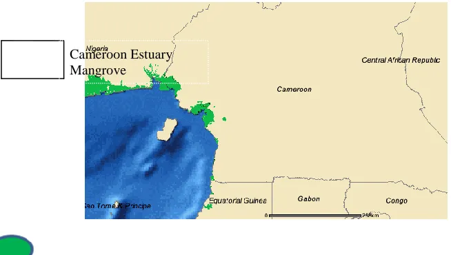
The coastal and marine environment of Cameroon forms part of the southern section of the Gulf of Guinea Large Marine Ecosystem [29], The coastline stretches from the Equatorial Guinea border at latitude 2° 30' N, to 4° 67' N at the Nigerian border and it is estimated at about 400 km in length [62]; [29]. The coastal area is approximately 9,670 km² [63] and is characterised by estuaries, coral and basalt rocks, sand and rock beaches, swamp and mangrove. About 30% of the coastline is covered with mangrove swamps [21]. The main Cameroon mangrove forests are found east and west of Mount Cameroon with smaller formations dispersed along the estuaries of the other rivers. The main stands of trees are the Rio-del-Rey and the Cameroon Estuary, respectively (Figure 1). The latter covers an estimated surface area of about 75,000 ha (approximately 50 km of coastline), while the former covers an estimated surface area of 175,000 ha (approximately 60 km of coastline from the River Sanaga to the Bimbia ______________________
Department of Environmental Science, University of
Buea, P.O. Box 63 Buea, Cameroon Tel +237(0)
74905963. E-Mail: [email protected]
Environment Department, University of York ,YO 105
138 estuary). The floristic composition of Cameroon mangrove
is characteristic of the Atlantic mangroves of West Africa. It is dominated by Rhizophora and comprises mostly three species, R. mangle, R. harrisonii and R. racemosa [21]. The pioneer species Rhizophora racemosa constitute 90-95% of the mangrove area, and may also form tall gallery forests in the Wouri estuary, reaching a height of 40 m, and colonizes recently deposited alluvial soils [30]. R. mangle and R. harrisonni are found in the drier, more saline landward edge of Rhizophora zones and between Rhizophora and Avicennia stands, but they rarely exceed 6m in height [30]. Other mangrove species include Avicennia germinans (black mangrove), which occurs on the higher elevation fibrous clay or sandier soils, Laguncularia racemosa and Conocarpus erectus (white mangrove), Acrostichum
aureum, Pandanus candelabrum and the introduced Nypa fruticans [21], [30]. Mangroves together with the coastal water (50m in depth) contain major fishery resources of significant economic importance. The annual fish production of both the Rio-del- Ray and Cameroon estuary is approximately 12,800 metric tonnes [47]. Scientific data about the Cameroon mangrove forest are limited. Threats to the system include forest resource exploitation, pollution from offshore oil exploration and large amounts of industrial effluent which drain into the mangrove forest. Assessment of the degree of dependency by the local community on the mangrove ecosystem shows that there is a high degree of interaction between the local residents and the mangrove forests, resulting in a significant level of dependency of the local communities on mangrove resources [46].
Sea Mangrove forest ______ International boundary
Figure 1: The Cameroon coastline showing stud y site (Adapted from UNEP –WCMC, 2005)
3 METHODS
The trophic interactions and energy fluxes of Cameroon estuary mangrove ecosystem were evaluated using Ecopath with Ecosim model for biomass estimations and consumption of different species groups within aquatic ecosystems [39],[38],[57],[35],[23],[11].. The model considers that all inputs are equal to the outputs for each species group through a series of simultaneous lineal equations, which for each functional group is expressed as: Biomass by (i) = all predation on (i) + non-predation biomass losses of (i) + export of (i) The terms in the equation may be replaced as follows:
Production by (i) = Bi. P/Bi
Predation biomass losses of (i) = ∑ (Bj. Q/Bi. DCji)
Other losses of (i) = (1-E Ei ) . Bi. P/Bi
For each component in the system, this leads to the linear equation
Bi. P/Bi . E Ei - ∑ (Bj. Q/Bi. DCji) - Ex –BAi = 0 Where,
t
i
B
andt
j
B
= are biomasses of prey (i) andpredators (j) respectively.
( / )
ti
P B
= Production /Biomass ratio, equivalent to total mortality (Z) of group i, in most circumstances.t
i
EE
= Ecotrophic Efficiency; the fraction of the total production of a group i, utilized in the system.(
Q
B
)
j = Consumption/Biomass ratio of group j,t
ji
DC
= fraction of i in the diet of predator j,t
i
EX
= exportof group i,
t
i
BA
= biomass accumulation of group i. All the variables are expressed at time t. Data requirements for Ecopath models are a minimum of three of the four following parameters for each group: Biomass (B), Production per unit biomass (P/B), Consumption per unit biomass (Q/B) and Ecotrophic efficiency (EE). Once the three parameters are entered for each group, the diet composition matrix is constructed (a diet matrix is constructed by indicating the percentage of each prey that occurs in each predator diet), and a balanced Ecopath model is obtained, several network parameters are evaluated, and these will determine the ecosystem‘s structure, maturity, and stability according to Odum [34], and hence reflect the system‘s ecosystem health [9]. Ecopath was modified several years ago with the inclusion139 of the dynamic simulation routines Ecosim [38],[57]. Ecosim
is a time-dynamic simulation model capability of Ecopath, for exploring past and future impacts, environmental disturbances, changes in predator-prey interactions and physiological behaviour due to mass changes. Ecosim comprises a series of differential equations [56]. The main equation is
i i i
ii j j i
B
e
F
M
I
Qij
Qji
gi
dt
dB
Where dBi/dt = growth rate during the time interval dt of group (i) in terms of its biomass Bi, gi is growth efficiency (production/consumption ratio), Fi is fishing (removal) mortality rate of group i, Mi = natural mortality rate (excluding predation) of group i, ei is emigration rate, Ii = immigration rate, and Qij (Qji) is the consumption rate of type i (j) biomass by type j (i) organisms. The consumption rates Qji are calculated based on the ‗foraging arena‘ concept, where the biomass of each prey i (Bi) is divided into vulnerable and an invulnerable components (Walters et al., 1997), and it is the transfer rate (vij) between these two parameters that determines if control is top-down ( Lotka– Volterra), bottom-up (donor-control) or an intermediate type . This will lead to the rate equation:
aijBj
ij
V
Vij
VijaijBiBj
Qij
b
Qij is the trophic flow of biomass per time between prey (i) and predator (j), Bi and Bj are the biomasses of prey and predators, respectively; aij is the rate of effective search for prey i by predator j, and Vij and Vb ij are prey vulnerability parameters, usually with default setting Vij = Vb ij. Parameters
Vij
andV
bij
represent prey vulnerabilities; it is the rate of exchange of biomass between two prey behavioral states: a state in which all predators have full access to prey and a state in which the prey have complete protection from predators. Thus, not all prey biomass is vulnerable to predation at any given time, and predator-prey relationships are limited by behavioral and physical mechanisms [56]. Ecosim is designed so that the user can specify the type of trophic control (Lotka-Volterra type vs donor control) that mediates any interaction in the food web. Maximum consumption rates are assumed. For low predator biomass or high prey vulnerability (Vij) the functional relationship is Lotka-Volterra type interaction (bottom-up) flows, which imply a strong ‗top-down‘ effect. For high predator biomass or low prey vulnerabilities the functional relationship approaches a donor-controlled (bottom-up) [56]. Prey vulnerabilities can be specified by adjusting the proportion of prey in vulnerable and invulnerable states. This is done by adjustment of the v values, which are scaled such that pure Lotka-Volterra type control = 1 and pure donor-control = 0. In the real world predator-prey interactions are characterised by this mixture of trophic control.3.1 Describing functional groups
To construct an Ecopath model, the first step is to define the functional groups. These can be based on ecological
similarities or function or a mixture of both. They can also be based on value-driven criteria, such as commercial status or importance to the local community. Functional groups can be individual species, size classes within species or broader taxonomic groupings. Due to extreme difficulties in parameterising some ecosystems to include all species, several food webs might be constructed for the same location depending on the information needed. Thus, for the Cameroon mangrove system, which has several hundred species, different versions of food web, differing in the number and kind of functional groups and complexity, could be constructed. For this study, the selection of functional groups to represent the Cameroon mangrove food web was a product of a collaborative process. A number of stakeholders and experts (including myself) participated in the discussion to produce functional groups based on the following criteria:
The species must be representative and abundant
The species must be relevant to the overall aims of the study
There must be some relevant data for those species (although not necessarily for the Cameroon mangrove forest).
In the final iteration, based on these criteria, 26 functional groups were selected for this model (Table 1): 13 fishes, 3 kinds of birds (11 species), groupings of 3 crabs, mangroves, phytoplankton, zooplankton, detritus, benthos, shrimps and insects. All the species within a functional group have ecological similarities, defined by similarities in diet, production and consumption rates, life history, and habitat associations, but also sometimes on value-driven criteria, such as commercial status or importance for subsistence users. Because of the nature of the Cameroon mangrove forest, where mangrove wood products are used extensively as source of energy to smoke fish, it is important therefore to consider the mangrove forest as a primary producer and make the link with fishing pressure. The functional group benthos was included because of its contribution to the diets of other groups.
Table1. Descriptions of some functional groups of the mangrove ecosystem in Cameroon.
_______________________________________________ 1. Mangrove Rhizophora spp., Avicennia spp, Laguncularia racemosa
2. Phytoplankton Diatoms, dinoflagellates and others 3. Zooplankton Neritic copepods, bivalve larvae, ostracods, mysids, nauplii, fish
eggs and others
4. Shrimps Peneaus spp, Parapenaeopsis atlantica, Penaeus notiali
5. Mangrove crabs Sesarmid species 6. Fiddler crabs Uca species,
7. Other crabs Scylla serrata, Cardisoma carnifex and
others 8. Ilisha africana
9. Pseudotolithus spp P. senegalensis, P. typus and P.elongates
140 12. .Brachydeuterus auritus
13. Dreprane africana
14. .Arius spp A . heudelotii and A. parkii 15. .Pomadasys jubelini
16. Galeoides decadactyl 17. Raja miraletus
18. Lutjanus spp L. goreensis and L. dentatus
19. Mugil curema
20. Caranx spp C. senegallus, C. hippo and C. senegalensis
21. Shorebirds Finfoot (Podica senegalensis ), Avocet (Recutrvirostra avosetta), White-footed plover (Charadrius marginatus),
Common Green shank (Tringa nebularia), Common sandpiper ( Actitis hypoleucos). 22. Birds of prey Black kite (Milvus migrans), Fish eagle (Haliaeetus vocifer), Palm nut vulture (Gypohierax angolensis), Harrier hawk (Polyboriodes typhus)
23. Insectivorous birds Grey flycatcher ( Musicapa cassini), Pied crow (Corvus albus) 24. Benthos
25. Insects
26. Detritus Organic matters and associated like bacteria
3.2 Ecopath input parameters
The input parameters for each group were: the biomass (B), the production/ biomass ratio (P/B), the consumption/ biomass ratio (Q/B) and ecotrophic efficiency (EE). Input parameters were estimated from the field or extracted from the literature, either from studies done within a similar mangrove ecosystem (in Central Atlantic region) or on the West Africa continental shelf. The diet matrix was constructed by designating the proportion of each prey that occurs in each predator‘s diet. Diets were derived mostly from the scientific literature, except for crabs groups where stomach content analysis had been carried out. The degree of confidence, that the parameters are appropriate for the Cameroon is expressed through the data pedigree coding option.
Mangrove
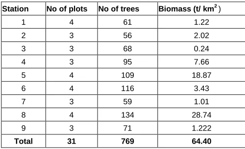
Mangrove above-ground biomass was estimated from 31 plots (each 10 m x 10m) using a plots method [14]. All trees within the plot were identified and the diameter at breast height (dbh) and height (h) was measured. The approach of Fromard [24] was used to calculate the above-ground biomass from diameter at breast height (dbh, in cm). Biomass (g) = a(dbh) b Where b and a are slope and intercept respectively .For Rhizophora species, b= 2.6, a = 128.2; For Laguncularia racemosa b =2.5, a=102.3 and; For Avicennia germinans b =2.4, a = 0.14. Total biomass (t/ km2) was then calculated by multiplication of the tree biomass by tree density (n/km2). Mangrove biomass calculated was 64.4 t/km2 .P/B values for mangrove were obtained from the literature (Table 2)
Table .2. Mangrove biomass estimate
Fish
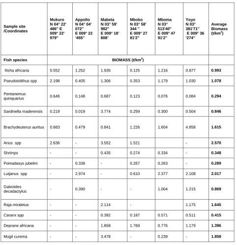
Data were obtained from six selected villages (Table 3) considered representative of the study area. These villages were selected because they were principal landing points, easy accessibility and village cooperation This fishery uses only dug-out canoes (3 to 7m in length), which are manually driven by one or two persons using a wooden paddle. The fishing gear is mainly gill net and line trap, the average mesh size is 60mm and an average area of 10.95 m2 (i.e. 7.3 m length and 1.5 m width). Generally, the fishermen leave the village early in the morning between 5am and 7.30am, depending on the weather and tidal amplitude, and return between 1pm and 3.30pm (fishing time approximately 8 hours), hauling is done manually for recovering the net and the entangled fish into the canoe. The sampling procedures were as follows: once the catch was landed on the village beach, I bought it. We then sorted out the fish into species and identified, counted and weighed. The fishes were then sold back to the fishermen. Additional information was gathered through interviews. Data collected were: (1) Fish catch identified to species level (2) Biomass of catch (total weight in kg) (3) Types of fishing gear used (4) Estimated area fished (km2). Fish biomass (Table 3) was estimated by ―sweep area‖ method used to determine the density of fish per square kilometre (Sherman, 1994). If the mean weight of catch is W, and A is the area swept, then: Fish density = W/A (kg/km2). W = the weight catch per month A = average area covered during fishing trip (approximately 6.7km2) Q = is efficiency of the net, or catchability coefficient, which represents the amount of the fish, caught by the fisherman relative to the amount that escaped being caught. In this case, Q was estimated as 60%. A1=is the whole area surveyed which is equal to the total water area (approximately 1500km2).
Biomass of fish = (W/A)/Q x A1
The P/B ratio (Table 4) of fish is equivalent to total mortality (Z) which is estimated as the sum of natural mortality (M) and fishing mortality (F):
Z = F+M
Natural mortality was calculated using the Von Bertalanfy growth function (VBGF):
Station No of plots No of trees Biomass (t/ km2 )
1 4 61 1.22
2 3 56 2.02
3 3 68 0.24
4 3 95 7.66
5 4 109 18.87
6 4 116 3.43
7 3 59 1.01
8 4 134 28.74
9 3 71 1.222
141
0.65 0.463
K
M
L
T
142 Table 3. Fish biomass estimates from six villages within the Cameroon mangrove system
Sample site /Coordinates
Mukuro N 04° 22' 486'' E 009° 22' 979''
Appollo N 04° 04' 072'' E 009° 22 '455''
Mabeta N 03° 59' 982" E 009° 18' 808''
Mboko N 03° 58' 344 '' E 009° 27 81'2''
Mboma N 03° 513'40'' E 009° 47 91'2''
Yoyo N 03° 381'71'' E 009° 36 '274''
Average Biomass (t/km2)
Fish species BIOMASS (t/km2)
Ilisha africana 0.552 1.252 1.935 0.125 1.216 0.877 0.993
Pseudotolithus spp 2.198 0.405 1.306 0.353 1.179 1.030 1.078
Pentanemus
quinquarius 0.646 0.148 0.687 0.123 0.076 0.084 0.294
Sardinella maderensis 0.219 0.019 3.774 0.259 0.300 0.504 0.846
Brachydeuterus auritus 0.683 0.479 0.841 1.226 1.604 4.858 1.615
Arius spp 2.636 - 3.552 1.521 - 2.570
Shrimps - - 0.435 0.274 0.334 - 0.348
Pomadasys jubelini - 0.338 - 0.267 0.263 - 0.289
Lutjanus spp - 2.974 - 0.610 2.377 2.108 2.017
Galeoides
decadactylus - 0.390 - - 1.004 1.215 0.869
Raja miraletus - - 2.114 - 1.175 1.645
Caranx spp - - 0.392 0.187 0.571 0.511 0.415
Deprane africana - - 1.858 1.769 0.776 1.179 1.396
143 Table 4 Natural and fishing mortality
Fish species Natural
mortality
Fishing mortality
Total
mortality Information sources
Ilisha Africana
L
= 22K
= 2.33 2.962 0.044 3.006 Fish base http://www.fishbase.org Pseudotolithus spp *L
= 67.18*K
= 0.25 0.508 0.140 0.648 [19]Pentanemus quinquarius
L
= 34K
= 1.081 1.592 0.183 1.775 Fish basehttp://www.fishbase.org Sardinella maderensis *
L
= 29.1*K
= 0.63 1.171 0.089 1.26 [19]Brachydeuterus auritus
L
= 20.6K
= 0.363 0.901 0.128 1.029 Fish basehttp://www.fishbase.org
Arius spp *
L
= 61.8*K
= 0.22 0.479 0.661 1.14 [19]Mugil curema
L
= 39.7K
= 0.68 1.1280.240 1.367
Fish base
http://www.fishbase.org
Pomadasys jubelini
L
= 45K
=0 .3 0.640 0.100 0.731 Fish basehttp://www.fishbase.org
Lutjanus spp 0.770 [3]
Galeoides decadactylus
L
= 54.5K
= 0.41 0.743 0.080 0.823 Fish basehttp://www.fishbase.org
Raja miraletus
L
= 87.9K
= 0.193 0.399 0.161 0.56 Fish basehttp://www.fishbase.org
Caranx spp 0.655 [49]
Drepane africana
L
= 40.1K
= 0.24 0.572 0.280 0.82 Fish basehttp://www.fishbase.org
Shrimps 5.380 [3]
*Average of different study from Djama [19]
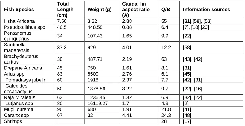
The Q/B ratios (Table 5) were estimated from the empirical relationship proposed by Palomares and Pauly [4]. Log Q/B = 7.964–0.204 log W∞–1.965T‘+0.083A+0.532h+0.398d
Where W∞ (or asymptotic weight) is the mean weight that the individuals of a population would reach if they were to grow indefinitely, T‘ is the mean environmental temperature expressed as 1 000 / (°C +273.15); A is the aspect ratio of the caudal fin, indicative of metabolic activity and expressed as the ratio of the square of the height of the caudal fin and its surface area; ‗h‘ and ‗d‘ are dummy variables, indicating herbivores (h=1, d=0), detritivores (h=0, d=1) and carnivores (h=0, d=0).
Table 5 Q/B ratio and sources of information
Fish Species
Total Length (cm)
Weight (g)
Caudal fin aspect ratio (A)
Q/B Information sources
Ilisha Africana 7.50 3.62 2.88 55 [31],[58], [53] Pseudotolithus spp 40.5 448.58 0.88 6.4 [7], [18],[20] Pentanemus
quinquarius 34 107.43 1.65 9.9 [22]
Sardinella
maderensis 37.3 929 4.01 12.2 [58]
Brachydeuterus
auritus 30 487.71 2.19 63 [43], [42]
Drepane Africana 45 750 1.61 8.1 [31]
Arius spp 83 8500 2.76 6.1 [45]
Pomadasys jubelini 60 1918 2.37 7.7 [42], [31] Galeoides
decadactylus 50 1378.86 3.22 9.7 [22], [16]
Raja Miraletus 63 1236.45 1.32 6.9 [32], [22]
Lutjanus spp 80 16119.27 1.7 4.3 [2]
Mugil curema 90 680 1.91 21.8 [41]
Caranx spp 67 32 4.41 24.3 [48]
Shrimps 28 [17]
Birds
Bird biomasses were estimated by multiplying the average wet weight of an adult of a given species by the average bird abundance [29]. Average bird abundance values were obtained from a study carried out in the Cameroon Rio del
144
Crabs
Crab biomasses were estimated using excavation and surface sample collection methods [28]. The crabs collected were sedated in ice water for a few minutes, washed and stored in 70% alcohol and later identified and weighed (wet
weighted) (Table 6). The P/B and Q/B ratios for these crabs were taken from literature (Table 8).
Table 6. Biomasses of crabs at stations studied
Station Average weight (g)
Sesarmid Fiddlers (Uca) Others
1 5.2005 0.707 1.22
2 2.826 2.319 0.55625
3
4.0499 1.13 0.611
4 4.767 1.146 0.864
5 5.13 1.763 0.951
6
7.2215 1.054 0.9625
7
3.441 1.523 3.399
8
4.319 1.7435 0.892
9 3.445 0.992 3.388
Average total weight 4.489 1.3755 1.427
Phytoplankton
Phytoplankton biomass was estimated from Froneman [24]. He reported chlorophyll a concentrations of 0.11 to 2.01 mg/l. This is equivalent to a water column concentration of 0.11 g/chl. To convert this to the standard unit of measurement used in the model (wet weight in t/km2 = g/m2), conversion factors reported in the literature were used. A factor of 25 was used to convert g chl a to g C, while the factors 2.5 and 5 were used to convert g C to g dry weight, then to g wet weight, respectively [36]. Phytoplankton biomass was thus approximately 34.4 t/km2. The P/B ratio of 180 was extracted from Wolff .[59].
Zooplankton
Zooplankton biomass was estimated from Froneman [24]. A mean biomass conversion ratio of 0.59±0.08 reported by Gate et al (1982), was used to convert dry weight to wet weight, hence zooplankton biomass was estimated at 27.13
t/km2. Also a P/ B ratio = 50 and a Q/B ratio = 160 were extracted from Wolff et al. [60].
Insects, Benthos and Detritus
145 Table 7. Biomass value for benthos and insects
Groups Biomass (t/km -2) Information sources
Benthos 4.593 [33]
Insects 0.61 [54]
Table 8. P/B and Q/B ratios
Group P/B Values Q/B Values Information sources
Mangrove 0.22 [59]
Phytoplankton 180 [59]
Zooplankton 50 160 [60]
Mangrove crabs (Sesarmidae) 2 14 [60]
Fiddler crabs (Uca) 5.5 95 [60]
Others crabs 0.25 22 [60]
Shorebirds 5.4 60 [3]
Birds of prey 0.1 65 [33]
Insectivorous birds 0.3 10 [60]
Insects 15.54 51 [54]
Benthos 12 20 [60]
3.3 Diet composition input data
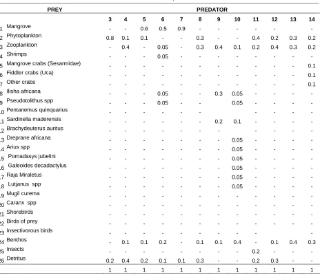
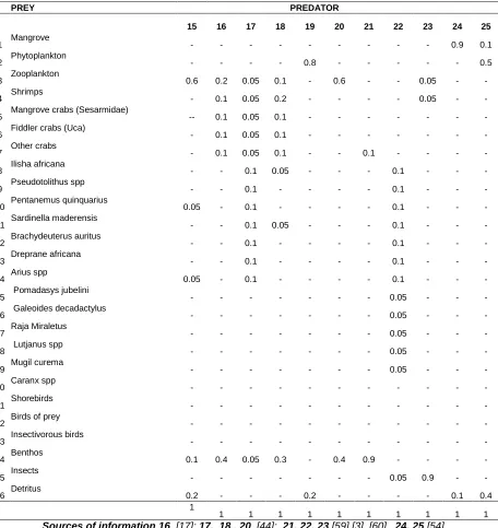
Diet information for crabs was obtained directly from stomach content analysis carried out back at the University of York. Literature data were used for all other functional groups (Table 9).
Table 9. Diet composition
Sources of information: 3 [59] 4 [33] 5, 6, 7 own estimates, 8 [53]; 9 [44]); 10 [17]; 11 [44]; 12. [6]; 13, 14 [17]) 15[33]
PREY PREDATOR
3 4 5 6 7 8 9 10 11 12 13 14
1 Mangrove - - 0.6 0.5 0.9 - - - -
2 Phytoplankton 0.8 0.1 0.1 - - 0.3 - - 0.4 0.2 0.3 0.2
3 Zooplankton - 0.4 - 0.05 - 0.3 0.4 0.1 0.2 0.4 0.3 0.2
4 Shrimps - - - 0.05 - - - -
5 Mangrove crabs (Sesarmidae) - - - 0.1
6 Fiddler crabs (Uca) - - - 0.1
7 Other crabs - - - 0.1
8 Ilisha africana - - - 0.05 - - 0.3 0.05 - - - -
9 Pseudotolithus spp - - - 0.05 - - 0.05 - - - -
10 Pentanemus quinquarius - - - -
11 Sardinella maderensis - - - 0.2 0.1 - - - -
12 Brachydeuterus auritus - - - -
13 Dreprane africana - - - 0.05 - - - -
14 Arius spp - - - 0.05 - - - -
15 Pomadasys jubelini - - - 0.05 - - - -
16 Galeoides decadactylus - - - 0.05 - - - -
17 Raja Miraletus - - - 0.05 - - - -
18 Lutjanus spp - - - 0.05 - - - -
19 Mugil curema - - - -
20 Caranx spp - - - -
21 Shorebirds - - - -
22 Birds of prey - - - -
23 Insectivorous birds - - - -
24 Benthos - 0.1 0.1 0.2 - 0.1 0.1 0.4 - 0.1 0.4 0.3
25 Insects - - - 0.2 - - -
26 Detritus 0.2 0.4 0.2 0.1 0.1 0.3 - - 0.2 0.3 - -
146 Table 9. Diet composition (continued)
PREY PREDATOR
15 16 17 18 19 20 21 22 23 24 25
1 Mangrove - - - 0.9 0.1
2 Phytoplankton - - - - 0.8 - - - 0.5
3 Zooplankton 0.6 0.2 0.05 0.1 - 0.6 - - 0.05 - -
4 Shrimps - 0.1 0.05 0.2 - - - - 0.05 - -
5 Mangrove crabs (Sesarmidae) -- 0.1 0.05 0.1 - - - -
6 Fiddler crabs (Uca) - 0.1 0.05 0.1 - - - -
7 Other crabs - 0.1 0.05 0.1 - - 0.1 - - - -
8 Ilisha africana - - 0.1 0.05 - - - 0.1 - - -
9 Pseudotolithus spp - - 0.1 - - - - 0.1 - - -
10 Pentanemus quinquarius 0.05 - 0.1 - - - - 0.1 - - -
11 Sardinella maderensis - - 0.1 0.05 - - - 0.1 - - -
12 Brachydeuterus auritus - - 0.1 - - - - 0.1 - - -
13 Dreprane africana - - 0.1 - - - - 0.1 - - -
14 Arius spp 0.05 - 0.1 - - - - 0.1 - - -
15 Pomadasys jubelini - - - 0.05 - - -
16 Galeoides decadactylus - - - 0.05 - - -
17 Raja Miraletus - - - 0.05 - - -
18 Lutjanus spp - - - 0.05 - - -
19 Mugil curema - - - 0.05 - - -
20 Caranx spp - - - -
21 Shorebirds - - - -
22 Birds of prey - - - -
23 Insectivorous birds - - - -
24 Benthos 0.1 0.4 0.05 0.3 - 0.4 0.9 - - - -
25 Insects - - - 0.05 0.9 - -
26 Detritus 0.2 - - - 0.2 - - - - 0.1 0.4
1
1 1 1 1 1 1 1 1 1 1
Sources of information 16 [17]; 17, 18 , 20 [44]; 21, 22, 23 [59],[3], [60] 24, 25 [54].
3.4 Balancing the model
After entering all the basic inputs into the Ecopath model, the first step is to check if the outputs are sensible, in other words, whether the biomasses of all groups can be supported by their consumption rates and the productivities of their prey. The initial model was unbalanced, as is usually the case in constructing any Ecopath model. The following steps were then taken to balance the model. 1. The ecotrophic efficiency for each group was checked
for inconsistencies, where the model calculated the EE
1. The biomass of some groups was adjusted, but not greater than 20% of the original input value. The basic empirical estimates for most parameters in the system remained unaltered. However, for the model to balance, specifying reasonable EE values for Shrimps, Pseudotolithius spp, Ilisha africana, Sardinella
maderensis and Pentanemus quainquarius was necessary because the biomasses of these groups needed to be otherwise adjusted by more than 40%. Ecotrophic efficiency is usually estimated by the program or assumed to be around 0.95 to 0.9 as proposed by Christensen et al. [13] in the Ecopath manual.
2. Diet composition for each group must sum to 1. 3. Data pedigree information was incorporated, which
147 different scopes for adjusting the data when
mass-balancing.
4. Sensitivity analysis was done to evaluate the accuracy of parameters estimated. Once the model was balanced, various ecosystem attributes were evaluated, these attributes include those given by Odum [34] and Christensen [10], allowing inferences to be drawn about the health of the ecosystem. A pedigree index of 0.52 was obtained from the model, implying that the model is of reasonable quality [12]. Using Ecosim, I changed the biomass of several groups to evaluate the effect of doing so on other species. The effect of changing mangrove biomass by 10%, 20% and 40% was evaluated on crabs and 10% to 80% for fish groups over a period of 20 years.
4 RESULTS
4.1 Structure and network analysis
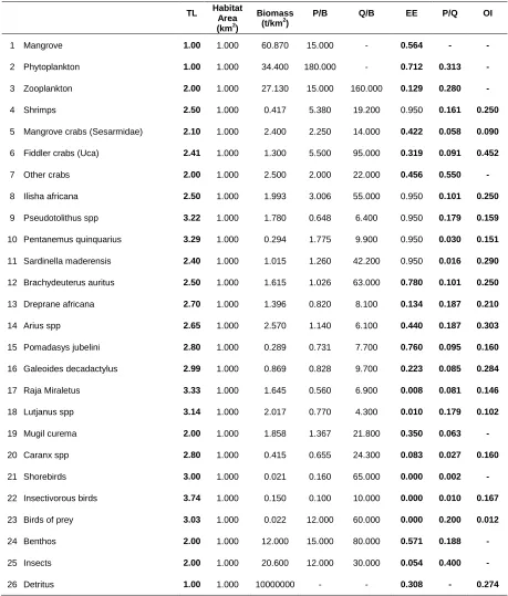
The balanced parameter estimates for the model are shown in Table 10. These parameters include trophic estimates, biomass estimates, production / biomass estimates, consumption /biomass estimates, production / consumption ratios, gross efficiency estimates and omnivory index estimates. The mangrove food web consists of 3 trophic levels and 17 sublevels, which range from 1.0 to 3.74 (Figure 2). The trophic level (TL) is an important index because it identifies an organism‘s food preferences. The highest values correspond to insectivorous birds, followed by the fish Pentanemus quinquarius and Pseudotolithus spp, whilst the lowest values correspond to the primary producer; mangrove, phytoplankton and detritus (Table 11).
Complexity in community structure
The omnivory index (OI) value is 0.143, which is quite low indicating a highly specialised consumer system. The low OI value may be due to some groups being highly specialized and environmental conditions might alter the availability of prey. An OI value of zero was estimated for zooplankton, which feed almost entirely on phytoplankton (80%), other crabs that feed almost on mangrove (90%), Mugil curema that feed virtually entirely on phytoplankton (80%), shorebirds that feed practically entirely on benthos (90%), insects that feed on mangrove (90%) and benthos that feeds mostly on detritus and phytoplankton (90%). The highest OI value of 0.450 was estimated for fiddler crabs, which take prey from many trophic levels (Table 12).
Community energetics
The energetic attributes of the ecosystem (Table 12) shows that the system mature and stability. These attributes include connectivity index (CI), total system throughput (T), system total primary production / total respiration ratio (PP/R), primary production / biomass ratio (PP/B), and biomass over throughput (B/T). The connective index (CI) is the number of actual links to the number of possible links for a given food web [11]. According to Odum [34] food web structure changes from linear to web like as the system mature. Hence, CI is correlated with maturity [11]. The Cameroon mangrove CI is 0.174 which is close to the value 0.191 reported by Villanueva [55] for Ebere lagoon in Ivory
148 Table 10. Basic input and model estimated output (bold) of the Cameroon mangrove estuary
TL Habitat Area (km2)
Biomass (t/km2)
P/B Q/B EE P/Q OI
1 Mangrove 1.00 1.000 60.870 15.000 - 0.564 - -
2 Phytoplankton 1.00 1.000 34.400 180.000 - 0.712 0.313 -
3 Zooplankton 2.00 1.000 27.130 15.000 160.000 0.129 0.280 -
4 Shrimps 2.50 1.000 0.417 5.380 19.200 0.950 0.161 0.250
5 Mangrove crabs (Sesarmidae) 2.10 1.000 2.400 2.250 14.000 0.422 0.058 0.090 6 Fiddler crabs (Uca) 2.41 1.000 1.300 5.500 95.000 0.319 0.091 0.452
7 Other crabs 2.00 1.000 2.500 2.000 22.000 0.456 0.550 -
8 Ilisha africana 2.50 1.000 1.993 3.006 55.000 0.950 0.101 0.250 9 Pseudotolithus spp 3.22 1.000 1.780 0.648 6.400 0.950 0.179 0.159 10 Pentanemus quinquarius 3.29 1.000 0.294 1.775 9.900 0.950 0.030 0.151 11 Sardinella maderensis 2.40 1.000 1.015 1.260 42.200 0.950 0.016 0.290 12 Brachydeuterus auritus 2.50 1.000 1.615 1.026 63.000 0.780 0.101 0.250 13 Dreprane africana 2.70 1.000 1.396 0.820 8.100 0.134 0.187 0.210
14 Arius spp 2.65 1.000 2.570 1.140 6.100 0.440 0.187 0.303
15 Pomadasys jubelini 2.80 1.000 0.289 0.731 7.700 0.760 0.095 0.160 16 Galeoides decadactylus 2.99 1.000 0.869 0.828 9.700 0.223 0.085 0.284 17 Raja Miraletus 3.33 1.000 1.645 0.560 6.900 0.008 0.081 0.146 18 Lutjanus spp 3.14 1.000 2.017 0.770 4.300 0.010 0.179 0.102 19 Mugil curema 2.00 1.000 1.858 1.367 21.800 0.350 0.063 - 20 Caranx spp 2.80 1.000 0.415 0.655 24.300 0.083 0.027 0.160
21 Shorebirds 3.00 1.000 0.021 0.160 65.000 0.000 0.002 -
22 Insectivorous birds 3.74 1.000 0.150 0.100 10.000 0.000 0.010 0.167 23 Birds of prey 3.03 1.000 0.022 12.000 60.000 0.000 0.200 0.012
24 Benthos 2.00 1.000 12.000 15.000 80.000 0.571 0.188 -
25 Insects 2.00 1.000 20.600 12.000 30.000 0.054 0.400 -
26 Detritus 1.00 1.000 10000000 - - 0.308 - 0.274
149
Table 11 Summary statistics and basic flows and indices
4.2 Simulated effects of mangrove biomass changes
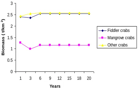
Simulations were done on 10%, 20%, 30% and 40% mangrove biomass changes. Figure 2a shows the crab biomass position within 20 years after simulation. The simulated effect of mangrove biomass changes on crabs was marked at 40% decline. The biomass of the entire crab declined within 5 years and then started to recover.The simulation is characterised by oscillations, with a maximum biomass reached at 18 years for most of the species (Figure 2b).
(a)
0 0.5 1 1.5 2 2.5 3
1 3 6 9 12 15 18 20
Years
B
io
m
a
s
s
(
t
/k
m
2)
Fiddler crabs
Mangrove crabs
Other crabs
Parameter Value Unit
Sum of all consumption 6723.632 t/km2.yr
Sum of all exports 3305.708 t/km2.yr
Sum of all respiratory flows 3810.424 t/km2.yr Sum of all flows to detritus 4775.025 t/km2.yr
Total system throughput 18615 t/km2.yr
Sum of all production 893 t/km
2
.yr Total net primary production 7105.1 t/km2.yr Total primary production/total respiration 1.865 t/km2.yr
Net system production 3294.4 t/km
2
.yr Total primary production/total biomass 38.6 t/km2.yr
Total biomass/throughput 0.01 t/km2.yr
Total biomass (excluding detritus) 184.2 t/km
2
.yr
Connectance index 0.3 t/km2.yr
System omnivory index 0.143 t/km2.yr
Ascendancy (flow bits) 9929.2
Relative ascendancy 0.25
Overhead (flow bits) 19117.1
Overhead (%) 48
Capacity (flow bits) 39661.3
Transfer efficiencies 6.3
Finn‘s cycling index (FCI %) 2
Finn‘s mean path length 1.717
Flow to detritus
Zooplankton 2050.348 t/km
2
.yr
Phytoplankton 1785.893 t/km2.yr
Mangrove 397.640 t/km2.yr
Insect 357.515 t/km
2
150 (b)
0 0.5 1 1.5 2 2.5 3
1 3 6 9 12 15 18 20
Years
B
io
m
a
s
s
(
t
/k
m
2)
Fiddler crabs Mangrove crabs Other crabs
Figure 2 (a). Original crab biomass over 20 years with unchanged mangrove biomass (b) Change in crab biomass with 40% change of mangrove biomass
The effect of changing mangrove biomass on fishes was explored. Figure 3 shows that fish biomass remained unchanged with mangrove biomass changes from 10% to 60%, but at 80% biomass change the effect was marked. The most affected species were Dreprane africana, Lutjanus spp, Pomadasys jubelini and Arius spp (Figure 4). It should be noted that there is no direct relationship between mangrove and fish, many intermediate trophic steps are involved.
0 0.5 1 1.5 2 2.5 3 3.5
1 3 6 9 12 15 18 20
Years
B
io
m
a
s
s
(t
/k
m
2)
Ilisha africana
Pseudotolithus spp
Sardinella maderensis
Brachydeuterus auritus
Arius spp
Dreprane africana
Pomadasys jub elini
Galeoides decadactylus
Raja Miraletus
Lutjanus spp
Mugil curema
Caranx spp
Figure 3 Original fish biomass over 20 years with unchanged mangrove biomass
4.3 Mixed trophic impact analysis
The mixed trophic impact analysis (Figure 5) assesses the direct and indirect impact of biomass change of one group on others. Bars above the line indicate a positive impact, whilst those below the line indicate a negative impact. Generally it can be seen that the pelagic groups will have the most impact on other pelagic groups. Mangrove, phytoplankton and zooplankton have positive impacts on most groups with Pseudotolithus spp have a large positive impact on Dreprane africana, Pomadasys jubelini and Galeoides decadactylus. While insectivorous birds positively impact the crabs and some
0 0.5 1 1.5 2 2.5 3 3.5
1 3 6 9 12 15 18 20
Years
B
io
m
a
s
s
(
(
t/
k
m
2)
Ilisha africana
Pseudotolithus spp
Sardinella maderensis
Brachydeuterus auritus
Arius spp
Dreprane africana
Pomadasys jubelini
Galeoides decadactylus
Raja Miraletus
Lutjanus spp
Mugil curema
Caranx spp
151 little or no negative impact. An increase in mangrove biomass has large positive impacts on the biomass of crab species, while they have little and no impact on other species. Fiddler crabs have positive impacts on Pentanemus quinquarius, Sardinella maderensis and Brachydeuterus auritus while they large negative impact on shrimps, Ilisha africana, Pseudotolithus spp, Dreprane africana, Pomadasys jubelini and Galeoides decadactylus. fish, they have largely negative impacts on Raja Miraletus, Lutjanus spp and Caranx spp.
Figure 5. Mixed trophic impact analyses for the Cameroon mangrove ecosystem. The bars show positive (above line) and negative (below line) impacts of each compartment. Impacted groups are shown along the horizontal axis and impacting groups
152 Figure. 6. Trophic interactions in the Cameroon mangrove. All the flows expressed in t/km2.yr. Each of the groups is placed on the Y-axis according to their trophic level. Biomass (B), Production (P), consumption (Q), the losses by respiration, the flows to
153
5 DISCUSSION
The parameter estimates of the programme appear reasonable. Model viability was determined by using the sensitive analysis function i.e. pedigree index [11]. Sensitivity analysis was done to evaluate the accuracy of parameters estimated, it suggests that parameterisation of groups within the model is most sensitive to decreases in biomass estimates and that the impact of changes in the parameters of one group on another is influenced by the trophic dependency of the impacting group on the impacted group. The impacts of an increase in biomass in one group on other groups within the systems can be shown using a mixed trophic impact plot (Figure 5). This can be used to get an overall indication of the sensitivities and responses to reduced biomass in one group on another and dependent upon them. The viability value of 0.52 estimated by the model is an indication that the model was tightly fitted, as the simulation values have remarkably little difference from the original input. The balanced model parameter estimates shown in Table 11 indicate a mixture of a mature and immature system. The mature indices include: total system throughput (T) that is the sum of all flows (consumption, respiration, export and flow into detritus) is 18,615 t/km2.yr, appears to be high when compared to other values from tropical coastal system . The system primary production/ respiration (PP/R) ratio estimated by the model is 1.87 (Table 11) indicating that the system is relatively developed [13]; the value is low when compared with other tropical ecosystems. The high ascendancy value of 9,929.2 and relative ascendancy of 0.250 indicate that the system is mature. However, the relative ascendancy of 0.250 reported by Vega-Cendejas and Arreguin-Sảnchez, [54] for Yucatan Peninsula (Mexico) was considered high by the author. The total system biomass value is 184.193 t/km2.yr which appears high fits well within the range of other tropical systems [12]. The model results show that more than 98.6% of the flows to detritus is from TL 1 and 2, these levels playing a significant role in supporting the energy utilised by higher TL groups, and indicate a detritus–based food web and bottom–top control system, which is typical of a mature system. System energy and matter recycling is an important process in ecosystem functioning [34], and the model low estimate of Finn‘s cycling index (FCI) and Finn‘s mean pathway of 1.983 and 1.717, respectively, is indicative of an immature system. The impact of mangrove change for the other functional groups was explored using the Ecosim routine and mixed trophic impact analysis (Figure 5). Mangroves have a positive impact on crab species and some other groups, with little negative or no impact on most species. A 40% change in mangrove biomass resulted to a drastic reduction in crab biomass (Figure 2b). The effect on fishes was obvious on four groups only, and at a high-level of mangrove biomass change (80%) (Figure 3). But modest changes in fish biomass were obvious for most fish groups, which suggest that mangrove is an important functional group for the system, though no direct trophic relationship exists with fishes. Mangroves play indirect role by producing detritus from the assimilation of fallen leaves within the sediment and detritus is utilised by many other groups in the food web or exported by tidal flush. The flows to detritus, from primary and second trophic levels, represent the main flow of energy in the food web.
REFERENCES
[1] Aguilar, B .J. 1999. Application of ecosystem health for the sustainability of managed system in Costa Rica. Ecosystem Health 5 (1):36-48.
[2] Allen, G.R. 1985. FAO species catalogue. Snappers of the world. An annotated and illustrated catalogue of Lutjanid species known to date. FAO Fish Synopium. 125(6):208-287pp.
[3] Amorim, P., G. Duarte, M. Guerra, T. Morato, and K. A. Stobberup. 2004. Preliminary Ecopath model of the Guinea-Bissau continental shelf ecosystem (NW Africa). 95-112 pp. In: Palomares, M.L.D., Pauly, D. (eds.) West African marine ecosystems: models and fisheries impacts. Fisheries Centre Research Reports 12(7). Fisheries Centre, UBC, Vancouver.
[4] Palomares, M.L.D., Pauly, D. 1998. Predicting food consumption 908 of fish populations as 909 functions of mortality, food type, morphometrics, temperature and salinity. Mar.910 Freshwater Res. 49, 447-453.
[5] Baird, D. and R. E. Ulanowicz. 1993. Comparative study on the trophic structure, cycling and ecosystem properties of four tidal estuaries. Marine Ecology Progress Series 99: 221-237.
[6] Ben-Tuvia, A. and R. McKay. 1986. Fishes of the north-eastern Atlantic and the Mediterranean. UNESCO, Paris. 2: 858-864pp
[7] Chao, L.N. and E. Trewavas. 1990. Check-list of the fishes the eastern tropical Atlantic (CLOFETA). UNESCO, Paris. 813-826 pp.
[8] George, Y., G.Y. Chiambeng, and H. J. Dumont. 2005. The Branchiopoda (Crustacea: Anomopoda, Ctenopoda and Cyclestherida) of the rain forests of Cameroon, West Africa: low abundances, few endemics and a boreal-tropical disjunction .Journal of Biogeography 32 (9): 1611–1620.
[9] Christensen, V. 1995. Ecosystem maturity towards quantification. Ecological Modelling 77:3-32.
[10] Christensen, V. and D. Pauly. 1992. Trophic Model of Aquatic Ecosystems. ICLARM Conference proceeding .
[11] Christensen, V. and C. J. Walters. 2004. Ecopath with Ecosim: methods, capabilities and limitations. Ecological. Modeling 172: 109-139.
[12] Christensen, V., C. J. Walters, and D. Pauly. 2004. Ecopath with Ecosim: a User‘s Guide. To be publish as Fisheries Centre reports, volume 12 (4), University of Columbia. Vancouver.15. (Available online at www.ecopath.org and www.fisheries.ubc.ca).
154 [14] Cintron, G. and N.Y. Schaeffer. 1984. Methods for
studying mangrove structure. 91-113pp. In Snedaker, S. C. & Snedaker J. G. (ed). The mangrove ecosystem research methods.UNESSCO , Paris France.
[15] Costanza, R. 1992. Toward an operational definition of health. In: Costanza, R., Norton, B., Haskell, B.D. (Eds.), Ecosystem Health—New Goals for Environmental Management. Inland Press, Washington, DC.
[16] Daget, J., J.C. Njock,.J. Daget, J. P. Gosse, and D.F. Thys Van Den Audenaerde. 1986. Check-list of the freshwater fishes of Africa (CLOFFA). Polynemidae. 352-354 pp. ORSTOM, Paris.
[17] Diallo, I., I. Cissé, and A. Bah. 2004. Modèle trophique du système système côtier du plateau continental Guinéen. 113-123pp .In: Palomares, M.L.D., Pauly, D. (eds.) West African marine ecosystems: models and fisheries impacts. Fisheries Centre Research.
[18] Djama, T. 1988. Estimation of growth parameters and mortality of longneck croaker (Pseudotolithus typus) in Cameroon.. FAO Fish. Report. 389:153-171.
[19] Djama, T. 2003. Biological parameters of some exploited fish species in the coastal waters of Cameroon. 58-61pp. In: M.L.D. Palomares, B. Samb, T. Diouf, J.M. Vakily and D. Pauly (eds.). Fish biodiversity: local studies as basis for global inferences. ACP-EU Fish Research Report.
[20] Etim, L. 2000. Length-weight relationship of eight fish species from the Cross River, Nigeria. Global Journal of Pure Apply Science. 6(4):571-575.
[21] Spalding, M., F. Blasco, and C. Field. 1997. World mangrove atlas. Okinawa, Japan: International Society for Mangrove Ecosystems
[22] Fiogbe, E.D. 2003. Morphometric relationships of commercially important fish species from Benin.. 25-30pp. In: M.L.D. Palomares, B. Samb, T. Diouf, J.M. Vakily and D. Pauly (eds.). Fish biodiversity: local studies as basis for global inferences. ACP-EU Fish research Report.
[23] Froese, R and D. Pauly. 2003. Fishbase. World Wide Web electronic publication http://www.fishbase.org.
[24] Froneman, P. W. 2001. Seasonal changes in zooplankton biomass and grazing in a temperate Estuary, South Africa. Estuarine, Coastal and Shelf Science 52:543–553.
[25] Fry, H. C., S. Keith, and E. Urban. 1982–2000. The birds of Africa. Vols 1–6. Academic Press, London.
[26] Fry, H. C., S. Keith, S., E. Urban, and M. Woodcock . 2004. The birds of Africa. Vols 7. Christopher Helm Press, London
[27] Gates, M., A. Rogerson, and J. Berger. 1882. Dry and wet weight biomass conversion constant for tetrehymena elliotti ( Ciliophora, Protozoa) . Oecologia 55: 145-148.
[28] Heymans, J. J. and D. Baird. 2000. A carbon flow model and network analysis of the northern Benguela upwelling system, Namibia. Ecological Modelling 126(1): 9-32. Price ARG, Klaus R, Sheppard CRC, Abbiss MA, Kofani M, Webster G (2000). Environmental and economic characterisation of coastal and marine system of Cameroon, including risk application of the Chad- Cameroon pipeline project. Aquatic Ecosyst. Health Manage., 3: 137-161
[29] Van Campo, E. and Bengo, MD. (2004). Mangrove palynology in recent marine sediments off Cameroon. Marine Ecology 208 (2-4): 315-330
[30] King, R.P. 1996. Length-weight relationships of Nigerian coastal water fishes. ICLARM. 19(4):53-58pp.
[31] McEachran, J. D. and K.A. Dunn. 1998. Phylogenetic analysis of skates, a morphologically conservative clade of elasmobranchs (Chondrichthyes: Rajidae). Copeia 2:271-290.
[32] Mendy, A. N. 2004. A trophic model of the Gambian continental shelf in 1986. 81-88pp. In: Palomares, M.L.D., Pauly, D.(eds.) West African marine ecosystems: models and fisheries impacts. Fisheries Centre Research Reports 12(7). Fisheries Centre, UBC, Vancouver.
[33] Odum, E. P. 1969. The strategy of ecosystem development. Science 164:262-270.
[34] Oritz, M. and M. Wolff. 2002. Dynamical simulation of mass-balance trophic models of benthic communities of north-central Chile: assessment of resilience time under alternative management scenarios. Ecological Modeling 148: 227-291.
[35] Parsons, T.R., Y. Maita, and C. M. Lalli. 1984. A manual of chemical and biological methods for eawater analysis. Oxford Pergamon Press.
[36] Pauly, D. 1980. On the interrelationships between natural mortality, growth parameter and mean environmental temperature in 175 fish stocks. ICES Journal of Marine Science 39: 175-192.
[37] Pauly, D., V. Christensen, and C. Walters. 2000. Ecopath, Ecosim, and Ecospace as tools for evaluating ecosystem impacts of fisheries. ICES Journal of Marine Science 57: 697-706.
155 [39] Rapport, D.J., R. Costanza, and A. J. McMicheal. 1998.
Assessing ecological health. Trend of Ecological Evolution 13:397-401.
[40] Robins, C.R. and G. C. Ray. 1986. A field guide to Atlantic coast fishes of North America.. Houghton Mifflin Company, Boston, U.S.A. 213-354 pp.
[41] Roux, C., J. Daget, J. P. Gosse and D.F. Thys Van Den Audenaerde .1986. Checklist of the freshwater fishes of Africa (CLOFFA). Pomadasyidae. 327-330pp. ISNB, Brussels; MRAC, Tervuren; and ORSTOM, Paris.
[42] Samb, B. 2003. On the biology of Brachydeuterus auritus from Senegalese waters. In M.L.D. Palomares, B. Samb, T. Diouf, J.M. Vakily and D. Pauly (eds.). Fish biodiversity: local studies as basis for global inferences. ACP-EU Fish Research Report. 14; 281pp.
[43] Samb, B. 2004. L‘écosystème sénégambien . In: Palomares, M.L.D., Pauly, D. (eds.).West African marine ecosystems: models and fisheries impacts. Fisheries Centre Research Reports 12(7). Fisheries Centre, UBC,Vancouver.
[44] Schneider, W. 1990. FAO species identification sheets for fishery purposes. Field guide to the commercial marine resources of the Gulf of Guinea. Prepared and published with the support of the FAO Regional Office for Africa. FAO, Rome. Longonje SN 2002. Utilisation of mangrove wood product amongst subsistence and commercial users. M.Sc thesis unpublished. Free University of Brussels (VUB).
[45] CWCS. 1997. Biodiversity conservation and management activities od Douala-Edea forest reserve. Finl technicl report for NC-IUCN, Amsterdam-Netherlands, Cameroon Wildlife Conservation Society (CWCS).
[46] Smith-Vaniz, W.F., J.C. Quéro, M. Desoutter,. J.C. Quero, J.C. Hureau, C. Karrer, A. Post, and L. Saldanha. 1990. Checklist of the fishes of the eastern tropical Atlantic (CLOFETA). Carangidae. 729-755pp. UNESCO, Paris.
[47] Stobberup, K.A., V. D. M. Ramos, and M. L. Coelho. 2004. Ecopath model of the Cape Verde coastal ecosystem. 39-56pp. In: Palomares, M.L.D., Pauly, D. (eds.) West African marine ecosystems: models and fisheries impacts. Fisheries Centre Research Reports 12(7). Fisheries Centre Vancouver.
[48] Thomas, J. 1995. Birds of the Rio del Rey estuary. Malimbus 17: 7-18.
[49] Ulanowicz, R. E. 1980. A hypothesis on the development of natural communities. Journal of Theoretical Biology 85: 223–245.
[50] Ulanowicz, R. E. 1986. Growth and development. Ecosystem phenomenology. Springer-Verlag, Berlin.
[51] Vkily, J.M. and A. Cham. 2003. Growth, feeding and reproduction of the West African Ilisha, Ilisha africana off Sierra Leone. p. 46-57. In: M.L.D. Palomares, B. Samb, T. Diouf, J.M. Vakily and D. Pauly (eds.). Fish biodiversity: local studies as basis for global inferences. ACP-EU Fish Research Report. 14. 281pp.
[52] Vega-Cendejas, M.E and F. Arreguín-Sánchez. 2001. Energy fluxes in a mangrove ecosystem from a coastal lagoon in Yucatan Peninsula, Mexico. Ecological Modelling 137: 119–133.
[53] Villanueva, M. C., P. Lal`ey`e, J. Albaret, R. Lae, L. Tito de Morais, and J. Moreau. 2006. Comparative analysis of trophic structure and interactions of two tropical lagoons. Ecological Modelling 197: 461-477.
[54] Walters, C., V. Christensen, and D. Pauly. 1997. Structuring dynamic models of exploited ecosystems from trophic mass balance assessments. Review in Fish Biology and Fisheries, 7(2):139–172.
[55] Walters, C.J., J. F. Kitchell, V. Christensen, and D. Pauly. 2000. Representing density dependent consequences of life history strategies in an ecosystem model. Ecosystems 3:70-83.
[56] Whitehead, P.J. 1985. FAO species catalogue. Volume.7. Clupeoid fishes of the world (suborder Clupeioidei). An annotated and illustrated catalogue of the herrings, sardines, pilchards, sprats, shads, anchovies and wolf-herrings. Part 1-Chirocentridae, Clupeidae and Pristigasteridae. FAO Fish. Synopium 125 (7):1-303.
[57] Wolff, M., V. Koch, J. B. Chavarria, and J. A. Vargas. 1998. A trophic flow model of the Golfo de Nicoya, Costa Rica. Revista de Biologia Tropical 46: 63–79.
[58] Wolff, M. K. and V. Isaac. 2000. A Trophic Flow Model of the Caete´ Mangrove Estuary (North Brazil) with considerations for the sustainable use of its resources. Estuarine Coastal and Shelf Science 50: 789–803.
[59] Xu.F.L. 1996. Ecosystem health assessment of Lake Chao, a shallow eutrophic Chinese lake. Lakes and Reservoir Research Management 2: 102-109.
[60] Sayer, J., C. Harcourt, and N. Collins., 1992. The conservation atlas of tropical forest-Africa. Macmillan publishing Limited. London.