Essays on Consumer Default

(1)

University of Pennsylvania

ScholarlyCommons

Publicly Accessible Penn Dissertations

1-1-2012

Essays on Consumer Default

Richard Grey Gordon

University of Pennsylvania, [email protected]

Follow this and additional works at:

http://repository.upenn.edu/edissertations

Part of the

Economics Commons, and the

Law Commons

This paper is posted at ScholarlyCommons.http://repository.upenn.edu/edissertations/512

For more information, please [email protected].

Recommended Citation

Gordon, Richard Grey, "Essays on Consumer Default" (2012).Publicly Accessible Penn Dissertations. 512.

(2)

Essays on Consumer Default

Abstract

Legislation dealing with consumer default has consistently struggled with an important trade-off: more debt forgiveness directly benefits households but indirectly makes credit more expensive. This dissertation assesses this trade-off in two ways and provides a tool for future research into this and other topics. Specifically, the first chapter analyzes how business cycles affect the positive and normative consequences of eliminating or restricting default, including the default restrictions put in place by the recent Bankruptcy Abuse Prevention and Consumer Protection Act of 2005 (BAPCPA). The second chapter examines the implications of

eliminating bankruptcy protection while still allowing households access to informal default. Lastly, the third chapter provides a novel tool for computing equilibrium in dynamic heterogeneous-agent economies, such as the economy in the first chapter.

There are four main findings. First, accounting for business cycles substantially reduces the welfare benefit of eliminating default. With or without business cycles, eliminating default greatly expands credit availability; however, when a protracted recession is possible, households use less credit unless they have a default option. Second, while business cycles reduce the welfare gain of eliminating default, this is not necessarily true for restricting default: BAPCPA significantly improves welfare whether or not aggregate risk is taken into account. Because the policy makes default more costly only for earnings-rich households, the reform improves credit markets while still preserving most of the insurance value of default. Third, eliminating bankruptcy protection leads to an increase in total defaults, debt, and welfare. Without bankruptcy protection, creditors can collect on defaulted debt to the extent permitted by wage garnishment laws. The elimination lowers the default premium on unsecured debt and permits low-net-worth individuals suffering bad earnings shocks to smooth consumption by borrowing. Last, the proposed computational method is capable of delivering a more accurate solution than the most widely used method and can be as efficient.

Degree Type

Dissertation

Degree Name

Doctor of Philosophy (PhD)

Graduate Group

Economics

First Advisor

Dirk Krueger

Keywords

Bankruptcy, Business Cycles, Computational Methods, Consumer Credit, Consumer Default, Garnishment

Subject Categories

(3)

ESSAYS ON CONSUMER DEFAULT Grey Gordon

A DISSERTATION in

Economics

Presented to the Faculties of the University of Pennsylvania in

Partial Fulfillment of the Requirements for the Degree of Doctor of Philosophy

2012

Supervisor of Dissertation

Dirk Krueger

Professor of Economics

Graduate Group Chairperson

Dirk Krueger

Professor of Economics

Dissertation Committee

Jes´us Fern´andez-Villaverde Satyajit Chatterjee

(4)

DEDICATION

(5)

ACKNOWLEDGEMENTS

This dissertation has benefited immensely from the supervision of Dirk Krueger who always was willing to help. Without the opportunity to work with Satyajit Chatterjee and have his guidance, the first two chapters of this dissertation would probably not have been written. Every suggestion Jes´us Fern´andez-Villaverde has made regarding this dissertation has strengthened it.

I have benefited from conversations with Aaron Hedlund, Pablo Guerron, Makoto Naka-jima, Burcu Eyigungor, Robert Hunt, Kurt Mitman, Andrew Clausen, Wenli Li, Greg Ka-plan, and Han Chen. I also received helpful comments from seminar participants at Indiana University, the University of Virginia, the University of Illinois at Urbana-Champaign, the University of Pittsburgh, the University of New South Wales, the Federal Reserve Bank of Cleveland, the Bank of Canada, the New Economic School, and Penn’s Macro Lunch Workshop.

(6)

ABSTRACT

ESSAYS ON CONSUMER DEFAULT Grey Gordon

Dirk Krueger

Legislation dealing with consumer default has consistently struggled with an important trade-off: more debt forgiveness directly benefits households but indirectly makes credit more expensive. This dissertation assesses this trade-off in two ways and provides a tool for future research into this and other topics. Specifically, the first chapter analyzes how business cycles affect the positive and normative consequences of eliminating or restricting default, including the default restrictions put in place by the recent Bankruptcy Abuse Prevention and Consumer Protection Act of 2005 (BAPCPA). The second chapter examines the implications of eliminating bankruptcy protection while still allowing households access to informal default. Lastly, the third chapter provides a novel tool for computing equilibrium in dynamic heterogeneous-agent economies, such as the economy in the first chapter.

(7)

List of Tables

1.1 Model Targets, Statistics, and Parameters . . . 22

1.2 Business Cycle Properties: Model and Data . . . 23

1.3 CD and ND Steady State Comparison . . . 25

1.4 CD and ND Aggregates and Change from Steady State . . . 30

1.5 Welfare Gains of Eliminating Default . . . 35

1.6 Welfare Gains of Making Default More Costly . . . 37

1.7 Effects of Policy Changes on Allocations . . . 39

1.8 Welfare Gains of the 2005 Reform . . . 41

1.9 Effects of Policy Changes on Allocations with Aggregate Risk . . . 42

1.10 Welfare Gains of the z-contingent Default Policy . . . 43

2.1 Model Statistics and Parameter Values . . . 62

2.2 Comparison of Baseline and Garnishment-Only Economies . . . 64

2.3 Wealth Distribution for Sweden: Data and Model . . . 69

2.4 Welfare Gains From Elimination of Bankruptcy . . . 70

2.5 Steady State Welfare Gains From Elimination of Bankruptcy . . . 71

3.1 OLG Calibration . . . 91

3.2 KS Calibration . . . 92

3.3 Error in the Law of Motion . . . 95

3.4 Euler-Equation Errors in the OLG Economy . . . 98

3.5 Running Times in Minutes for the OLG Economy . . . 100

(10)

3.7 Simulated Capital Sequence Comparison . . . 102

3.8 Law of Motion Forecast Errors in the KS Economy . . . 102

A.1 Cyclical Properties of Chapter 7 Filings per Household . . . 118

A.2 US Business Cycle Properties (1960-2004) . . . 118

A.3 Parameter Values for Profiles . . . 120

A.4 Law of Motion Forecasting Accuracy . . . 122

A.5 Contribution of Business Cycle Components to Welfare Results . . . 123

A.6 Robustness to Guaranteed Income . . . 124

A.7 Robustness of Results to Alternative Retirement Schemes . . . 126

A.8 Robustness of Results to Flat Profiles . . . 127

A.9 Robustness of Results to Flexible Portfolios . . . 128

C.1 Accuracy of the Law of Motion . . . 141

C.2 Accuracy of the Policy Functions . . . 141

(11)

List of Figures

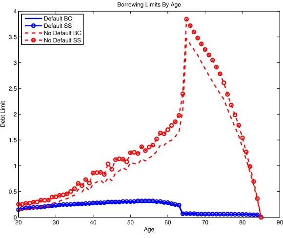
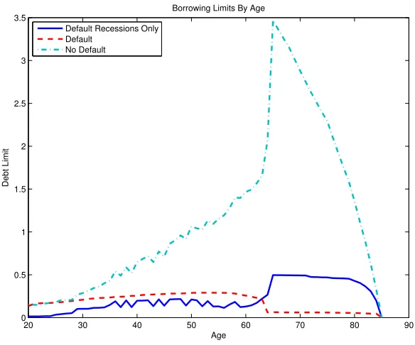
1.1 Borrowing Limits in the Default and No Default Economies . . . 26

1.2 Log Consumption in Steady State . . . 27

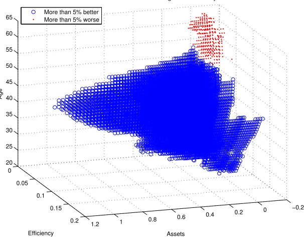
1.3 Welfare Gains of Eliminating Default By Age in Steady State . . . 29

1.4 Borrowing Limits with and without Aggregate Uncertainty . . . 31

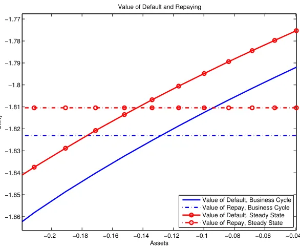
1.5 Value from Default and Repayment . . . 33

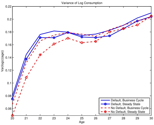
1.6 Variance of Log Consumption By Age . . . 34

1.7 Welfare Gain By Age with and without the Business Cycle . . . 35

1.8 Business Cycle Effect on Welfare Gain of Eliminating Default . . . 36

1.9 Borrowing Limits with the BAPCPA Reform . . . 41

1.10 Borrowing Limits with Default in Recessions Only . . . 43

2.1 Value Functions . . . 67

2.2 Loan Supply in the Baseline and Garnishment-Only Economies . . . 68

2.3 Mean Consumption by “Age” . . . 72

2.4 Dispersion of Consumption by “Age” . . . 73

3.1 Capital Stock Forecasts forT = 3 . . . 96

3.2 Today vs Tomorrow’s Capital Stock forT = 3 . . . 97

3.3 Simulated Capital Sequence Comparison . . . 102

A.1 Chapter 7 Filings Per Household (1960-2010) . . . 116

(12)

Chapter 1 Evaluating Default Policy: The

Business Cycle Matters

Grey Gordon

Summary

(13)

with-out the business cycle. Moreover, with the policy instituted, eliminating default produces a welfare loss of .1%, which aggregate risk deepens to 1.5%. The reform improves credit markets while still preserving most of the insurance value of default. A different type of policy that restricts default to only be in recessions or expansions sharply reduces welfare relative to always allowing default (a loss of 1.4%) or never allowing it (a loss of 1.9%). The policy introduces uncertainty that makes credit expensiveand keeps households from relying on the default option.

1.1 Introduction

In both recent and past history, the merits and flaws of legislation dealing with consumer default have been subject to intense debate.1Central to the arguments has been the trade-off between debt relief and credit.2 _{More debt relief directly benefits households but indirectly}

harms them through reduced access to credit: to cover losses due to default, creditors must charge a premium. Complicating the issue is that the circumstances of unfortunate debtors are often caused by events outside their control. Panics, financial crises, stock market crashes, and housing busts can leave otherwise prosperous, stable households in financial ruin.

The interaction between aggregate risk and consumer default is particularly relevant in light of recent US history. Preceded by twenty years of stable economic growth, the Bankruptcy Abuse Prevention and Consumer Protection Act of 2005 made debt-forgiveness significantly more difficult.3 Since then the economy has slipped into the most severe reces-sion since the Great Depresreces-sion. Far from being just coincidence, this sequence of events fits into a pattern where legislation responds to negative aggregate shocks with more debt

1

Bankruptcy laws changed frequently prior to 1900 and even since then have had major revisions in 1938, 1978, and 2005. Bankruptcy in its present form did not take shape until 1898, and even then it was highly controversial with efforts to repeal it made in 1903, 1909, and 1910 (Warren,1935, p. 143).

2

For instance, one Senator argued for a bill he introduced in 1885 saying, “At present interest rates . . . are from 8 to 20%, because of the doubt whether the creditor will have his fair share of the estate . . . ” (quoted in Warren, 1935, p. 133). Another Senator argued against the bill saying, “it is no time to pass bills of this character—when every man in trade . . . is suffering from the depression . . . ” (quoted inWarren,

1935, p. 132).

3_{The key provision of the reform is that households with above-median income may no longer file for}

(14)

relief and to positive shocks with less.4 Was the 2005 reform beneficial in light of the last recession? Would it have been if the economy had remained stable? How does law changing in response to aggregate shocks impact households? More generally, how does aggregate risk affect the welfare consequences of eliminating or restricting default? This paper seeks to answer these questions.

I find aggregate risk substantially decreases the welfare benefit of eliminating default. In a calibrated general equilibrium life-cycle model and absent aggregate risk, eliminating default improves welfare by 1.8% of lifetime consumption for newborn households. Once a business cycle—the type of aggregate risk considered in this paper—is added, this gain drops to .5%. Eliminating default in either the steady state or business cycle environment means that creditors offer any amount of debt at a risk-free rate. For their part, households avoid taking out debt beyond what they can repay with probability one. This amount is much smaller in the business cycle because of the possibility, albeit remote, of a life-long recession which would severely depress aggregate capital and wages. With a default option, credit is more expensive and less abundant, but households can safely use all of it by defaulting if a protracted recession hits.

While including aggregate risk reduces the welfare gain of eliminating default, I find this need not be the case when restricting default. I consider two cases of default being restricted. First is a policy change designed to mimic the 2005 reform by forcing households with above-median earnings to repay a substantial fraction (but not all) of their debt. This reform increases welfare by around 2% with or without the business cycle. Further, with the reform instituted, households experience a welfare loss from eliminating default: .1% absent aggregate uncertainty and 1.5% with it. The reform increases repayment rates of the earnings rich, those with the greatest ability to repay, resulting in a large expansion of credit. At the same time, most of the insurance value of default is preserved: all households have access to some amount of default and earnings-poor households can easily default. This

4

I thank Satyajit Chatterjee for pointing this out to me. A recent example of this pattern, besides the 2005 reform, is the Emergency Economic Stabilization Act of 2008—passed in response to the latest recession—that authorized an ongoing mortgage-modification program (the Home Affordable Modification Program). There are also many older examples where “prosperity muted demands for relief” until a panic, drought, or war “eased . . . opposition to a bankruptcy law” (Coleman,1974, p. 24, 28).Robe, Steiger, and

Michel(2006) argue from a broad historical perspective that default penalties become lighter as risk becomes

(15)

result suggests that “default” is not a problem but rather the amount of default allowed. The second type of default restriction I consider is meant to capture aggregate risk’s effect on legislation by only allowing default in recessions or expansions. Surprisingly, the outcome of either policy is inferior to always having default (a loss of 1.4%) or never having it (a loss of 1.9%). The reason for this is that uncertainty about whether or not default will be allowed has two negative effects. First, it causes creditors to charge a default premium which households must always pay.5_{Second, households must be prepared to never have the}

default option by limiting the amount of debt they take on. Consequently debt is expensive

and households cannot rely on the default option.

Most research suggests that eliminating default would substantially improve welfare in the absence of uninsured “disaster” states.6 The result has proven surprisingly robust. In particular, it has been found in both partial and general equilibrium environments, for finitely-lived and infinitely-lived households, under different informational settings, and un-der alternative debt-pricing formulations.7In addition,Athreya et al.(2009b) find the result holds for numerous specifications of earnings risk and preferences. Further,Chatterjee and

Gordon (2011) consider multiple alternatives to bankruptcy law and find one that

com-pletely eliminates default is optimal. To my knowledge, the only exception in the literature is the work byLi and Sarte(2006) that shows accounting for general equilibrium effects can reduce the welfare benefit of eliminating default even to the point of making it a loss.8 A central contribution of the present paper is to show that aggregate risk is also an important determinant of the welfare consequences of eliminating default.

Research on the welfare gains of restricting access to default is more mixed and has focused on the 2005 reform. Athreya (2002), Li and Sarte (2006), and Nakajima (2008) have found modest changes in welfare and allocations from the reform.9_{Chatterjee, Corbae,}

5

Consistent with the rest of the literature default premiums are paid upfront. If the premiums were chargedonly after the aggregate state was revealed, this effect would not be present.

6

Examples includeAthreya(2002),Livshits, MacGee, and Tertilt(2007),Athreya(2008),Athreya, Tam,

and Young(2009a),Athreya, Tam, and Young(2009b), andChatterjee and Gordon(2011).

7

Throughout the paper “partial equilibrium” refers to allowing default-risk premia to adjust while holding fixed default-risk-free prices at the equilibrium values in the default economy. In the business cycle model this requires using the law of motion from the default economy to forecast prices.

8

One potentially important caveat is that none of these papers have computed the transition.Chatterjee

and Gordon (2011) compute the transition for eliminatingbankruptcy—the focus of their paper—but not

for eliminatingdefault.

(16)

even-Nakajima, and R´ıos-Rull(2007) andMitman(2011), on the other hand, have found sizable welfare gains. None of these papers have allowed for aggregate risk, and a contribution of the present paper is to take aggregate risk into account in studying how the 2005 reform— passed just before the Great Recession—affected households. I show that the reform likely made them better off. Another contribution of the paper is to examine default policy that restricts or permits default in response to aggregate shocks. I show that such a policy can be very harmful to households.

Little quantitative work has been done on default and business cycles. Nakajima and

R´ıos-Rull(2004) andNakajima and R´ıos-Rull(2005) examine whether bankruptcy amplifies

or smooths aggregate shocks. In the first paper, the authors use a production economy where creditors make profits or losses and distribute them via a dividend. In the second, the authors use a storage economy but impose a special timing on the model to ensure creditors make zero profits loan-by-loan.10 While these papers examine default’s effect on aggregate dynamics, the present paper examines the effect of aggregate dynamics on default. Consequently, they are complementary. A technical contribution of the paper is to model the economy with aggregate uncertainty in a way that ensures creditors make zero profits loan-by-loan without imposing a special timing. This is done by allowing some households to have adjustable portfolios and offset losses from charge-offs.

The quantitative framework I use is an extension ofChatterjee et al.(2007) andLivshits

et al. (2007) to include aggregate uncertainty. Recessions are modeled as a negative shock

to total factor productivity, a large increase in earnings variance a laStoresletten, Telmer,

and Yaron (2004), and a decline in exogenous labor supply (which is calibrated to match

the standard deviation of hours worked). General equilibrium and the life-cycle are both included as the work of Li and Sarte (2006) and Livshits et al. (2007) suggests these are very important for evaluating default policy. Following Athreya et al. (2009b), I abstract from expenditure shocks (large negative shocks to asset positions).11

tually become part of the Bankruptcy Abuse Prevention and Consumer Protection Act of 2005.

10

Specifically, households must make their default decisions before the aggregate shock is realized.

11

Livshits et al.(2007) have argued that expenditure shocks are quantitatively important for the

(17)

In a series of robustness exercises, I find the result that aggregate risk substantially

reducesthe welfare gain of eliminating default is quantitatively robust. Specifically, it is true for different earnings processes, mortality risk profiles, and economies of scale in household size. It is also true when a substantial portion of labor income is guaranteed. Further, the result holds even if default is not completely eliminated but just made very costly. While the reduction in the welfare gain is robust, thelevel of the welfare gain is not robust and can vary greatly. This is especially true when a substantial portion of earnings is guaranteed. In this case, the welfare gain from eliminating default can be significantly lower after including aggregate risk but still be very high in absolute terms.

The rest of the paper is organized as follows. Section 1.2 describes the models with and without aggregate uncertainty. Section 1.3 discusses the calibration and baseline model properties. Section 1.4 examines the consequences of eliminating default. Section 1.5 ex-amines the consequences of restricting default. Section 1.6 concludes. Appendices include extended model and data descriptions, notes on computation, and robustness exercises.

1.2 Model

I first lay out the model without aggregate uncertainty and then modify it to include aggregate uncertainty. Time is discrete in both models.

Steady State Model

The steady state model is a completely standard model of consumer default with general equilibrium and the life cycle.

Demographics, Endowments, Technology, and Preferences

The economy is populated by a unit mass of households who die with certainty afterT years. Households are endowed with one unit of time but differ in the productive efficiency e of

(18)

their time endowment and in certain other characteristicss,including age. Characteristics lie in a finite setSand evolve according to a Markov chainF(s0|s).12Efficiency is distributed iid conditional on characteristics according to a density functionf(e|s) which has support inR++ for all s.

Households face an age-dependent conditional probability of survival ρs. Households

who die are replaced by “newborn” households having zero assets, efficiency distributed according to ˆf(e|s), and characteristics distributed according to ˆF(s). The utility from death is normalized to zero.

Preferences over consumption are given by

T X

t=1

βt−1U(ct, st) (1.1)

whereβ >0 is the discount factor andc is consumption. The period utility function is

U(c, s) = (c/θs)1−σ/(1−σ), σ >0, σ6= 1. (1.2)

where θs is the age-dependent effective number of household members.13 When σ = 1,

U(c, s) = log(c/θs). Households do not value leisure.

A neoclassical production firm operates the production technology KαN1−α with α ∈

(0,1) that uses as inputs capital K rented at rate r and labor N hired at wage w. Capital depreciates at a constant rateδ∈(0,1).

Legal Environment

The legal environment is designed to resemble Chapter 7 bankruptcy in US law. Households have a credit historyh∈ {0,1}. Households in good standing,h= 0, have the right to file for bankruptcy. If they do, three things happen in the filing period: their debts are discharged in exchange for all their assets, they may not save and may not borrow, and a fraction

χ ∈ [0,1) of their income is given to creditors.14 In the period after filing, a household’s credit history records that they filed for bankruptcy in the past, h = 1. This record is

12_{Age evolves deterministically so that, if} _t₍_s_{) denotes the age of a household,} _F₍_s0

|s) = 0 whenever

t(s0)6=t(s) + 1 (except ift(s) =T in which case the transition is immaterial).

13_Since _σ_{will be 2 in the calibration,}_θ

s will shift marginal utilities in the same way as in, for instance,

Attanasio and Weber(1995) andGourinchas and Parker(2002).

14_{There are a number of reasons to believe} _some _{income is transferred to creditors in the period of}

(19)

removed and their history showsh= 0 with probability 1−λ. For as long as a household is in bad standing, h = 1, a household is not allowed to borrow but may save.15 Households begin life withh= 0.

Asset Markets

Households do not directly hold claims to capital, but rather enter into debt or savings contracts with a financial intermediary who owns the capital stock and rents it to the production firm. I now describe these contracts.

From a household’s perspective, a debt/savings contract looks just like a risk-free dis-count bond. The face valuea0 lies in a finite set Athat includes zero and both positive and negative elements. I use the convention a0 ≥0 denotes savings and a0 <0 denotes borrow-ing. Because of default, each contract has a potentially different yield and so has a distinct priceq(a0, s) that varies with all factors that can potentially influence next period’s default decision. Sinceeis iid conditional ons, these are entirely summarized in characteristicss.16 The pricesq(a0, s) for a0∈A, s∈S define a “price schedule.”

From the intermediary’s perspective, a debt/savings contract is a repayment agreement that through pooling gives a certain return. In exchange for q(a0, s)a0 of the consumption good, the intermediary expects a yieldρsp(a0, s)a0 next period comprised of two parts. First,

from households surviving to the next period, he expects to recover only p(a0, s) ∈ [0,1] fraction of the debt because some may default. Second, he expects that only ρs fraction of

households will survive to even have a chance of repaying.

In addition to contracts, the intermediary (but not households) has access to two other assets, capital and a risk-free discount bond. The bond B0 has price ¯qB and capital K0 has

return 1 +r−δ. Capital cannot be short sold and the bond is in zero net supply. Note that no arbitrage necessitates the bond’s return be equated to the return on contracts. This pins

the bankruptcy code incorporates “good faith” requirements that are not explicitly modeled here. Second, earnings are sometimes garnished before households file for bankruptcy with one estimate in Chatterjee

and Gordon(2011) putting the net recovery rate on defaulted revolving debt at around 15%. Third, some

households initially file for Chapter 13 (which results in a debt repayment plan) but subsequently file for Chapter 7.

15

Musto(2004) finds credit opportunities are severely restricted while the record of a bankruptcy remains.

16

The contract can be made contingent on (a, e, s, h). However since the default decision next period is a function of (a0, e0, s0, h0), onlya0andsmatter. The credit history doesn’t appear inq(a0, s) because debt,

(20)

down the price schedule as

q(a0, s) = ¯qBρsp(a0, s) (1.3)

fora06= 0. Without loss of generality, q(0, s) is taken to be zero.

The Household Problems

The household problems are as follows.17 Let V(a, e, s, h) denote the value function of a household. A household in good standing h= 0 that can repay their debt solves

V(a, e, s,0) = max

d∈{0,1}(1−d)·V

R₍_{a, e, s}_{) +}_d_·_VD₍_{e, s}₎ _(1.4)

where the value of repaying is

VR(a, e, s) = max

c,a0 U(c, s) +βρsEV(a

0_{, e}0_{, s}0_,₀₎

c+q(a0, s)a0 =we+a

c≥0, a0∈A

(1.5)

and the value of defaulting is

VD(e, s) = max

c,a0 U(c, s) +βρsEV(0, e

0_{, s}0_,₁₎

c=we(1−χ)

c≥0, a0 = 0.

(1.6)

A household in good standing that cannot repay their debt must default. A household in bad standing h= 1 solves

V(a, e, s,1) = max

c,a0 U(c, s) +βρsλEV(a

0

, e0, s0,1) +βρs(1−λ)EV(a0, e0, s0,0)

c+q(a0, s)a0 =we+a

c, a0 ≥0, a0∈A.

(1.7)

Let the policy functions be denotedd(a, e, s, h),a0(a, e, s, h),c(a, e, s, h), where a household in bad standing is said to not default, i.e. d(a, e, s,1) = 0.

17

(21)

The Intermediary’s Problem

Details of the intermediary’s problem are in Appendix A.1. The intermediary maximizes the net present value of financial income using contracts, capital, and the bond. He is indifferent over all feasible allocations if contracts are priced according to (1.3) and if capital’s return equals the bond’s return.

Equilibrium

I now give a simplified definition of equilibrium. An unsimplified definition, along with the characterizations that lead to this definition, are given in Appendix A.1.

A steady state equilibrium is a collection of pricesr, w, q, recovery rates p, policy func-tionsc, a0, d, a value functionV, a strictly positive capital stockKand labor supply N, and a distribution of householdsµ such that all of the following hold:

1. The policies and value function solve the household problems.

2. The capital stock and aggregate labor supply are given by the distribution:18

K =∫(a+d(a, e, s, h)(−a−χwe))dµ/(1 +r−δ) (1.8)

N =∫edµ. (1.9)

3. Prices satisfy

q(a0, s) = ¯qBρsp(a0, s) (1.10)

¯

qB= 1/(1 +r−δ) (1.11)

r =α(K/N)α−1 (1.12)

w= (1−α)(K/N)α. (1.13) 4. Repayment probabilities are consistent: for all a, s−1,

p(a, s−1) =

X

s Z

(1−d(a, e, s,0) +d(a, e, s,0)χwe/(−a))f(e|s)deF(s|s−1). (1.14)

5. The distribution is invariant to household policies and stochastic transitions.

18

(22)

Business Cycle Model

I now modify the steady state model to include aggregate uncertainty. The model is setup recursively using S = (z, µ) as the aggregate state where µ is a distribution of households and z is a productivity shock. The aggregate state evolves according to a law of motion Γ with S0

z0 = Γ(z0,S) denoting next period’s aggregate state conditional on a z0 realization.

Further, I use G= Γ(g,S) andB= Γ(b,S) to denote the states that will arise conditional on ag orb realization.

Demographics, Endowments, Technology, and Preferences

The production technology is nowzKαN1−α. The productivity shockztakes on one of two possible values inZ ={g, b} withg > b and evolves according to a Markov chain F(z0|z). Capital is rented at rater(S) and labor is hired at wagew(S). As before, capital depreciates at a constant rateδ.

The household efficiency process is now allowed to vary with the aggregate state. Specif-ically, eis drawn from f(e|s, z) ands evolves according to F(s0|s, z0). Similarly the distri-butions for newborn households are ˆf(e|s, z) and ˆF(s|z).

Household preferences over consumption are the same as before and leisure is still not valued. The assumptions on preferences, mortality risk, and endowments imply an exoge-nous stochastic process for aggregate labor supply N. It is assumed that the labor supply conditional onz0=gis always weakly larger than the labor supply conditional on z0 =b.

Legal Environment

The legal environment is the same as in steady state.

Asset Markets

(23)

productivity shock isz0. The price of a z0-contingent contract is denotedqz0(a0, s;S). Hence

there are two price schedules,qg(a0, s;S) and qb(a0, s;S).

From the intermediary’s perspective, a contract costs qz0(a0, s;S)a0 and gives a certain

yield ρsp(a0, s;S_z00)a0 contingent on a z0 realization. The recovery rate p(a0, s;S_z00) reflects

that not only may households default, but that their decision depends on the aggregate stateS_z00.

As before, the intermediary has access to capital K0 and a risk-free discount bond B0

with price ¯qB(S). Additionally, and following Krusell, Mukoyama, and S¸ahin (2010), the

intermediary has access to an “aggregate complete” set of Arrow securities A0_g and A0_b

with prices ¯qg(S) and ¯qb(S). Because capital’s return is risky and the bond’s return is

risk-free, these Arrow securities are redundant when the short-sale constraint on capital is not binding.19 All assets except capital are in zero net supply.

With the aggregate-complete set of Arrow securities, contract pricing is simple. Because a z0-contingent contract can be replicated by a z0-contingent Arrow security, no arbitrage dictates that

qz0(a0, s;S) = ¯q_z0(S)ρ_sp(a0, s;S0

z0) (1.15)

fora0 6= 0. Without loss of generalityqz0(0, s;S) = 0. This shows the price ofz0-contingent

contract reflects the cost of transferring resources to that state ¯qz0(S), the probability of

survivalρs, and the recovery rate p(a0, s;S_z00) conditional on reaching that state. This

con-tract pricing ensures that there is no cross-subsidization across different loan types and is therefore consistent with free entry by intermediaries.

While contracts are priced in this independent fashion, household access to these con-tracts is restricted. Specifically, a household of typesmust choose (a0_g, a0_b) from a setP(s).20 In the calibrated model, there will be two groups of households separated, essentially, into the bottom 80% of labor income earners and the top 20%. The bottom 80% will have access to a fixed portfolio which for the sake of simplicity and clarity is a bond.21 For

19_{Recall next period’s labor supply is assumed to be weakly larger if}_g_{is realized than}_b_{is realized. This,}

together withg > b, ensures r(G)> r(B) so that capital is indeed risky.

20_{I assume}_A+_×_A+_⊂_P₍_s_{) for some}_s_{having ˆ}_F₍_s_|_z₎_>_{0 for each}_z_and_T _≥_{2. This technical assumption}

ensures some positive measure of households can always be incentivized to increasea0g (in the aggregate) or

a0b by varying ¯qg and ¯qb. 21

(24)

them P(s) = {(a0_g, a0_b) ∈ A ×A|a0_g = a0_b}. The top 20% on the other hand will have access to a bond for borrowing but can save using any (a0_g, a0_b) combination. For them

P(s) = {(a0_g, a0_b) ∈ A×A|a0_g = a0_b ifa0_g < 0 or a0_b < 0}. These portfolio restrictions are similar to the ones in Chien, Cole, and Lustig (2011) where 10% of the population has freely adjustable portfolios, 20% use a fixed, weighted portfolio of bonds and equity, and the remaining 70% use a bond.

The portfolio restrictions are meant to capture that while a large menu of tradeable assets is available, only rich households seem to use them.22In particular,Kennickell(2009) demonstrates that the top 20% of the income distribution (and especially the top 5%) hold a disproportionate share of their portfolio in businesses and other non-housing wealth while the bottom 80% hold primarily housing wealth.23 Moreover, Campbell (2006) shows the portfolios of households with the least assets contain virtually only safe ones.24 Together with the observation that interest on consumer credit is almost always tied to the prime rate (and not, for instance, the return on equity), the assumed portfolio restrictions seem plausible. That said, there will in general be large welfare gains from removing these portfolio restrictions. In Appendix A.4, I show one of the main results, that aggregate risk reduces the welfare gain of eliminating default, holds when there are no portfolio restrictions.

The Household Problems

LetV(a, e, s, h;S) denote the value function of a household. Taking the law of motion and

prices as given, households solve the following problems.

A household in good standing h= 0 that can repay its debt solves

V(a, e, s,0;S) = max

d∈{0,1}(1−d)·V

R₍_{a, e, s}_;_S_{) +}_d_·_VD₍_{e, s}_;_S₎

(1.16)

(1 +r(Sz00)−δ)k0for some k0 and eachz0, has three advantages. First, it is consistent with the theoretical

structure of the model (whereAis a fixed set). Second, in the computation it avoids interpolating the value function and price schedules in theadirection. Third, it allows for the natural borrowing limit to be written down in a straightforward fashion.

22_{While imposing exogenous portfolio restrictions to capture this endogenous outcome is not ideal, it}

seems reasonable given that the model abstracts from informational costs and other potential barriers to entry in financial markets.

23_{See p. 25 and Figure 27 of his paper.}_Carroll₍₂₀₀₀_{) documents a similar fact for the wealth distribution.} 24

(25)

where the value of repaying is

VR(a, e, s;S) = max

c,a0 g,a0b

U(c, s) +βρsEV(a0z0, e0, s0,0;S_z00)

c+qg(a0g, s;S)a

0

g+qb(a0b, s;S)a

0

b =w(S)e+a

c≥0,(a0_g, a0_b)∈P(s)

(1.17)

and the value of defaulting is

VD(e, s;S) = max

c,a0 g,a0b

U(c, s) +βρsEV(0, e0, s0,1;Sz00)

c=w(S)e(1−χ)

c≥0,(a0_g, a0_b) = (0,0).

(1.18)

A household in good standing that cannot repay its debt must default. A household in bad standing h= 1 solves

V(a, e, s,1;S) = max

c,a0 g,a0b

U(c, s) +βρsλEV(az00, e0, s0,1;S_z00)

+βρs(1−λ)EV(az00, e0, s0,0;S_z00)

c+qg(a0g, s;S)a

0

g+qb(a0b, s;S)a

0

b =w(S)e+a

c, a0_g, a0_b ≥0,(a0_g, a0_b)∈P(s).

(1.19)

Let the associated policy functions be denotedd(a, e, s, h;S),a0_z0(a, e, s, h;S),c(a, e, s, h;S)

where a household in bad standing is said to not defaultd(a, e, s,1;S) = 0.

The Intermediary’s Problem

Details of the intermediary’s problem may be found in Appendix A.1. Essentially, the inter-mediary maximizes the net present value of financial income discounted by Arrow security prices ¯qz0(S). He does so using contracts, capital, a risk-free bond, and the two Arrow

se-curities. He is indifferent over all feasible allocations if contract prices satisfy (1.15) and if

1 = ¯qg(S)(1 +r(G)−δ) + ¯qb(S)(1 +r(B)−δ)

¯

qB(S) = ¯qg(S) + ¯qb(S).

(1.20) These are equivalent to

¯

qg(S) = (1−q¯B(S)(1 +r(B)−δ))/(r(G)−r(B))

¯

qb(S) = (¯qB(S)(1 +r(G)−δ)−1)/(r(G)−r(B)).

(26)

While not immediately apparent, the presence of adjustable portfolios permits the fi-nancial intermediary to make zero profits in every state (not just in expectation). A proof of this fact is given in Appendix A.1.25 Because the intermediary makes zero profits, a theory of how any gains or losses are distributed across households does not need to be developed.

Equilibrium

I now give a definition of equilibrium that has been substantially simplified. The unsimplified definition, as well as the characterizations leading to it, are in Appendix A.1. A recursive competitive equilibrium is a collection of price functionsr, w,q¯g,q¯b,q¯B, qg, qb, recovery rates

p, policy functions,c, a0_g, a0_b, d, a value function V, a capital stockK and labor supplyN as functions of the aggregate state, and a law of motion Γ such that the following hold:

1. The policies and value function solve the household problems.

2. The aggregate capital stock and labor supply are given by the distribution and the capital stock is strictly positive:

K(S) =∫(a+d(a, e, s, h;S)(−a−χw(S)e))dµ/(1 +r(S)−δ)>0 (1.22)

N(S) =∫edµ. (1.23)

3. Prices satisfy

qz0(a0, s;S) = ¯q_z0(S)ρ_sp(a0, s;S0

z0) (1.24)

¯

qg(S) = (1−q¯B(S)(1 +r(B)−δ))/(r(G)−r(B)) (1.25)

¯

qb(S) = (¯qB(S)(1 +r(G)−δ)−1)/(r(G)−r(B)) (1.26)

r(S) =zα(K(S)/N(S))α−1 (1.27)

w(S) =z(1−α)(K(S)/N(S))α. (1.28)

25_{Intuitively, for zero profits to obtain, the intermediary’s capital income must exactly offset his contract}

obligations. This implies contract obligations must have an identical return structure to capital. In general, there will not exist a fixed portfolio of assets that will deliver this because the presence of default makes contract obligations, and in particular charge-offs, vary in a non-trivial way. By allowing flexible portfolios, some households can be induced to change the ratioa0g/a0bin the aggregate and so make contract obligations

and capital have the same return structure. This is accomplished by varying the bond price ¯qB, which

(27)

4. Repayment probabilities are consistent: for all a, s−1 andS, p(a, s−1;S) =

X

s Z



 

1−d(a, e, s,0;S)+

d(a, e, s,0;S)χw(S)e/(−a)





f(e|s, z)deF(s|s−1, z). (1.29)

5. All asset markets clear and the intermediary makes zero profits which is equivalent to (1 +r(B)−δ)X

a0 Z

ρsp(a0, s;G)a01[a0=a0g(a, e, s, h;S)]dµ

= (1 +r(G)−δ)X

a0 Z

ρsp(a0, s;B)a01[a0=a0b(a, e, s, h;S)]dµ.

(1.30)

6. The law of motion is consistent with stochastic transitions and household policies. The least obvious equation is (1.30). This ensures the only asset the intermediary needs to use (besides contracts) is capital. To see this, suppose there was no mortality risk, no default, and that portfolios mimicked capital,a0_z0 = (1 +r(S_z00)−δ)k0 for somek0 and each

z0. In this case, (1.30) becomes

(1 +r(B)−δ)∫(1 +r(G)−δ)k0dµ= (1 +r(G)−δ)∫(1 +r(B)−δ)k0dµ (1.31) which always holds. To carry household savings into the next period, all the intermediary must do is choose capital holdingsK0 equal to ∫k0dµwhich makes the bond and Arrow se-curities unnecessary. With default, mortality risk, and flexible portfolios, some adjustments must be made to reflect that savings are contingent and that only the aggregate portfolio must resemble capital.

The only “deep” prices in the model are the factor prices, r and w, and the risk-free discount bond price ¯qB. Essentially by no arbitrage, the Arrow security prices ¯qg,q¯b and

price schedules qg, qb can be written as functions of these, as is evident when looking at

equations (1.24),(1.25), and (1.26). The bond price is used to clear the asset markets, as summarized in equation (1.30), by controlling the relative cost of saving using a0_g versus using a0_b.26

26_{Importantly, as ¯}_q

B approaches 1/(1 +r(B)−δ) from above, the Arrow price ¯qg and hence the price

schedule qg approach zero. This makes saving usinga0g become arbitrarily cheap driving up the left hand

side of (1.30). At the same time, the Arrow price ¯qb approaches 1/(1 +r(B)−δ) meaning saving usinga0b

does not become arbitrarily cheap. This keeps the right hand side of (1.30) bounded from above. As ¯qB

(28)

1.3 Calibration and Baseline Properties

This section discusses the calibration and baseline model properties. The model period is a year.

Functional Forms

I first describe the functional form for the efficiency process and then for portfolio availabil-ity.

Efficiency

I select the efficiency process to capture three potentially important features of the data. First is that earnings persistence and variance change over the life cycle. This feature is demonstrated inKarahan and Ozkan(2010) where it is shown earnings shocks are less per-sistent early in life. In the model, persistence and contract pricing are tightly linked, so this could prove important. Second is that the variance of persistent earnings shocks increases in recessions and decreases in expansions as demonstrated inStoresletten et al. (2004). As default provides a way of intratemporally smoothing consumption, this fluctuation in in-tratemporal dispersion could also prove important. Third is that the earnings distribution has a thick right tail. By selecting an efficiency process that generates this right tail, the model will also be able to match the concentration of wealth in the data. This is important because the wealthiest households will not be directly affected by default policy. Conse-quently, general equilibrium effects of changes in default policy would likely be overstated were these households missing.

To account for these features of the data, I use two efficiency processes with working households stochastically transitioning between them, as well as a separate process for retirement. The efficiency process for the majority of working households and all newborns is governed by

eh,z =ψzφhexp(uh+εh)

uh =γhuh−1+ηh,z, u0 = 0

ηh,z∼N(0, σ2η,h,z), εh ∼N(0, σε,h2 )

(29)

wherehdenotes age. This process has a deterministic componentφh, a persistent component

uh, a transitory component εh, and an “aggregate labor supply shifter” ψz. As labor is

supplied inelastically, the supply shifter is used to match the cyclical volatility of hours worked.27 Note that the persistence is governed by γh which is age-dependent, as are the

variances of the persistent and transitory shocks. Also note the variance of the persistent shockσ_η,h,z2 is a function of z (the steady state variance is σ2_η,h,₁).

While most working households use this “log process,” they have a probabilityπbw(bw

for “blue to white” collar) of transiting to the process

eh,z=ψzφhυ

υ∼

υ−υ

¯

υ−υ

ξ

with support [υ,υ¯].

(1.33) This “super rich” process also has an aggregate, deterministic, and transitory component, however the transitory component is drawn from a different distribution governed by three parameters,υ,υ,¯ andξ. The functional form for theυdistribution is taken fromChatterjee

et al. (2007) who in the spirit of Casta˜neda, D´ıaz-Gim´enez, and R´ıos-Rull (2003) posit a

low-probability state where earnings are very high but transitory. AsChatterjee et al.(2007) argue, such a state provides households with the “opportunity and incentive” to accumulate large amounts of wealth.28 Households revert to the log process with probability πwb and

draw uh from N(0, σ2η,1,z) and εh from N(0, σε,21).29 The transition is deterministic (i.e. πwb= 1) in the last period of working life.

When households retire, their efficiency is30

eh,z =κFψzφJexp(uJ) +κGψz (1.34)

whereJ is the first period of retirement. This retirement process is very similar to the one

inLivshits et al.(2007) andAthreya et al.(2009a). The proportional componentκF reflects

27_{Note that the literature tends to focus on residual earnings, i.e. what is left after running a first-stage}

regression on log earnings using a complete set of time dummies. The model process is consistent with this in that running such a regression would remove ψz (and the wage w) which will be common across all

households.

28

The only way to equate marginal utilities, given the high income and transitory nature of the state, is to save a large amount. In the calibration, the iid assumption onυ, together with a large value for ¯υand a small value forξ, delivers this.

29_{They draw from the distribution for newborn households both for simplicity and because the peristent}

variance is large (reflecting a large cross-sectional variance of the persistent shock).

30_{I follow}_{Krusell, Mukoyama, S}_{¸ahin, and Smith}₍₂₀₀₉_{) and model retirement income as home production}

(30)

earnings made over a household’s lifetime, and the guaranteed component κG provides

a fraction of average earnings. Mean efficiency is normalized to one in steady state. By assumption all households are under the log process in the last period of working lifeJ−1 and take one last draw ofη to arrive atuJ.

Portfolio Availability

Recall that the portfolioP(s) available to households is allowed to vary with their character-isticss. I now let P(s) equal{(a0_g, a0_b)∈A×A|a0_g =a0_b ifa_g0 <0 or a0_b <0}for “super-rich” households and P(s) equal {(a0_g, a0_b) ∈ A×A|a0_g = a0_b} for all others.31 This means the typical household will use only a risk-free bond, but a few earnings-rich households will, in addition to a risk-free bond, have access to freely adjustable portfolios for savings.

Parameter Values and Baseline Properties

For the steady state calibration, I adopt most targets and many parameters fromChatterjee

et al.(2007). The coefficient of relative risk aversion σ is 2. The capital share of incomeα

is 0.36 and the depreciation rate of capital δ is .10. The average duration of a bad credit record 1/(1−λ) is taken to be ten years implyingλ= 0.9. Wealth and earnings targets are reported in Table 1.1. I target a debt-output ratio of .0067 and a fraction in debt of 6.7. For the filing rate, I target .50%.32

Households begin life at age 20, begin retirement at 65, and live to at most 85. The profiles of residual earnings persistence and variance (γh, ση,h,2 1, σε,h2 ) are the non-parametric

estimates ofKarahan and Ozkan(2011).33The persistenceγhbegins low at around .7 before

increasing to unity by age 40 and mostly staying there until retirement. For countercyclical earnings variance, there are no age-specific estimates available, so I use estimates from

31_{The technical assumption on}_P₍_s_{) dictates some}_>_{0 measure of households is born super rich.} 32

This is the average number of filings per household from 1999-2003, .93%, prorated to only account for the number of filings due to earnings shocks which Chatterjee et al. (2007) put at 53.5% based on

Chakravarty and Rhee(1999). The literature has used a wide range of targets from .29% inChatterjee et al.

(2007) to 1.2% inAthreya et al.(2009a).

33_{The sample in}_{Karahan and Ozkan}₍₂₀₁₁_{) is for ages 24 to 60 and I use nearest-neighbor extrapolation}

(31)

Storesletten et al. (2004) assuming the ratio ση,h,g/ση,h,b is age-independent and equal to

.59 and that .5ση,h,b+.5ση,h,g = ση,h,1.34 The retirement parameters (κF, κG) are set to

(.35, .15) giving an average replacement rate of roughly 50%.35The deterministic component of efficiency φh and mortality risk profile ρs are calibrated using estimates from Hubbard,

Skinner, and Zeldes (1994).36 The earnings profile φh follows a hump-shape over the life

cycle, nearly doubling from age 20 to its peak at age 48 before almost returning to its age-20 value by retirement. The effective household-size profile θs is calibrated using the “mean”

equivalence scale inFern´andez-Villaverde and Krueger (2007) and the profile of household size calculated from the CPS by Bick and Choi (2011).37 All the profiles are reported in Appendix A.2.

The productivity process is assumed to be symmetric with an expected duration of expansions and recessions at 3 years. This implies F(g|g) = F(b|b) = 2/3. A standard deviation of 2.24% is targeted for the Solow residual implying the technology shock takes on

g= 1.0224 orb= 0.9776.38The aggregate labor supply shifterψz is calibrated, once the rest

of the calibration is set, to match the 1.74% standard deviation of log hours worked reported

inCasta˜neda, D´ıaz-Gim´enez, and R´ıos-Rull (1998). This results in (ψg, ψb) = (1.025, .975)

with the steady state valueψ1 normalized to 1.

There are 7 remaining parameters: 1 preference parameter β, 1 technology parameter

χ, and 5 efficiency-process parameters (υ,υ, ξ, π¯ bw, πwb). These are used to minimize the

weighted distance between the steady state model and target statistics. The steady state model is computed with grid search and backward induction in Fortran. For details of the

34_{The value of}_σ

η,g/ση,b is .59 inStoresletten et al.(2004). 35

AlthoughAthreya et al.(2009a) andLivshits et al.(2010) set (κF, κG) = (.35, .2), they do not have the

earnings rich. The lower value forκG(the guaranteed portion ofmeanearnings) of .15 reflects a mean/median

income that is approximately 75% of its value when including the income-rich (roughly 1.2 compared to 1.6).

36

Hubbard et al. (1994) estimate separate deterministic profiles for household heads with less than 12

years of education (NHS), 12-15 years (HS), and 16+ years (COL) of education. I average the profiles of these three types for the year 1986 assuming 13% of the population is NHS, 48% is HS, and 39% is COL. This breakdown of educational attainment is from the 2010 Current Population Survey for ages 30-34 (see Table 1 athttp://www.census.gov/hhes/socdemo/education/data/cps/2010/tables.html).

37_{Specifically, I assume}_θ

s=f(Ns) whereNs is the average number of household members andf is the

mean equivalence scale inFern´andez-Villaverde and Krueger (2007) linearly-interpolated to be continuous. The values for θs are very similar to the ones in Livshits et al. (2007). The benchmark calibration

over-predicts the hump in consumption, but in a robustness exercise I show θs = 1 makes the results even

stronger (see Appendix A.4 Table A.8). This suggests estimatingθsto match the consumption profile would

not significantly alter the results.

38

(32)

computation see Appendix A.3.

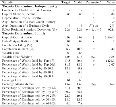
The results from the calibration are listed in Table 1.1. The model does fairly well at reproducing the targets. Specifically the right tails of both the earnings and wealth distri-butions are matched closely as is the capital-output ratio. As in virtually all the bankruptcy literature, the calibration has difficulty jointly matching the filing and debt statistics.39 Hav-ing some income transferred to creditors in the period of default (via the default cost χ) helps a lot in matching these statistics, as does some flexibility with the efficiency process.

The model with aggregate uncertainty is computed using the method of Krusell and

Smith (1998). The distribution is summarized with two of its moments, aggregate wealth

and labor supply, and an equity premium is included as a state variable.40 The household problem is solved with grid search, backward induction, and linear interpolation of the aggregate moments. For results to be comparable between the steady state and business cycle versions, the same number and placement of grid points are used in both models (in both the asset and efficiency direction). The model is simulated non-stochastically as

in Young (2010), and the asset markets are cleared in each period of the simulation. The

resulting approximate law of motion makes accurate price forecasts 1-step ahead with R2

values above .997 and maximum errors below .13% as well as 50-steps ahead withR2 values above .995 and maximum errors below .37%. For additional details, the reader is referred to Appendix A.3.

Table 1.2 reports the cyclical properties of the model and US economies with a discussion of the levels of model aggregates deferred to the next section. The data are described in Appendix A.2. Filings are too volatile and too countercyclical; however, default in the model is based entirely on earnings shocks. Other reasons for default, such as divorce, health bills, and lawsuits, are probably not as correlated with the business cycle nor as volatile. The volatility of consumption is too low. The labor supply volatility is exactly as targeted, and

39

Three approaches have been used to try to overcome this problem. First is the approach used by

Chatterjee et al. (2007) and S´anchez (2007) who calibrate the earnings process to match some earnings

statistics. Second is the approach used in Athreya et al.(2009b) who take estimates from the literature but use a stochastic punishment for default. Third is the approach used inLivshits et al.(2007) who take estimates from the literature but make debt partially secured through a “garnishment” technology and posit transaction costs for debt. The approach I use here is a mixture of the first and the third.

40_{Including an equity premium as a state variable is fairly common in the literature. For instance,}

Storesletten, Telmer, and Yaron (2007) include ES(R(Sz00))−q¯B(S)−1. The benefit of doing this is that

(33)

Statistic Target Model Parameter* Value

Targets Determined Independently

Coefficient of Relative Risk Aversion 2 2 σ 2 Capital Share of Income .36 .36 α .36 Depreciation Rate of Capital .10 .10 δ .10 Avg. Duration of a Bad Credit History 10 10 λ .9 Avg. Duration of a Business Cycle 3 3 F(z|z) 2/3 Solow Residual Standard Deviation (%) 2.24 2.24 g−1,1−b .0224

Targets Determined Jointly

Capital-Output Ratio 3.08 3.08 ξ 1.59e-3 Debt-Output Ratio ×100 .67 .69 χ .12 Population Filing (%) .50 .18

Population in Debt (%) 6.7 10.5 β .940

Wealth Gini .80 .83

Wealth Mean/Median 4.03 4.13 πwb .588

Percentage of Wealth held by Top 5% 57.8 69.5 υ¯ 1429.3 Percentage of Wealth held by Top 20% 81.7 83.6 υ 2.67 Percentage of Wealth held by 40-20% 12.2 9.8

Percentage of Wealth held by 60-40% 5.0 4.9 Percentage of Wealth held by 80-60% 1.3 1.8

Earnings Gini .61 .50

Earnings Mean/Median 1.57 1.59 πbw .153

Percentage of Earnings held by Top 5% 31.1 30.5 Percentage of Earnings held by Top 20% 60.2 55.4 Percentage of Earnings held by 40-20% 22.9 19.1 Percentage of Earnings held by 60-40% 13.0 12.5 Percentage of Earnings held by 80-60% 4.0 7.8 *Parameters are listed beside statistics they strongly influence.

Table 1.1: Model Targets, Statistics, and Parameters

output and investment are close to their US counterparts. Output is persistent but not as persistent as in the data.

1.4 Eliminating Default

Overall, the calibrated model is broadly consistent with US data. I now explore the conse-quences of eliminating default both in terms of welfare and allocations, and see how these change in the presence of aggregate risk.41 The benchmark economy, that is the one with

41_{I do not account for the transition, and there are two reasons for this. First is that when a policy change}

(34)

Stdev x Stdev x/ Correlation of lagged x with y Variable (x) in (%) Stdev y x(−2) x(−1) x x(+1) x(+2)

US (1960-2004)

Output (y) 2.44 1.00 0.01 0.58 1.00 0.57 -0.01 Consumption 1.69 0.69 0.02 0.59 0.92 0.59 0.10 Investment 7.19 2.94 0.04 0.53 0.89 0.38 -0.26 Hours Worked 1.60 0.66 -0.23 0.26 0.82 0.69 0.09 Defaulting Pop 10.25 4.20 0.17 0.00 -0.03 0.26 0.56

Model

Output (y) 2.96 1.00 -0.10 0.08 1.00 0.08 -0.09 Consumption 0.82 0.28 -0.28 -0.11 0.84 0.45 0.23 Investment 8.14 2.75 -0.05 0.12 0.99 -0.01 -0.16 Labor Supply 1.74 0.59 0.03 0.18 0.95 -0.14 -0.26 Defaulting Pop 12.34 4.17 0.27 0.15 -0.69 -0.21 -0.42 Debt* 6.54 2.21 0.28 0.25 0.08 -0.79 -0.58 Population in Debt* 4.50 1.52 0.29 0.25 0.07 -0.83 -0.54 *Debt is negative net worth. US counterparts to my knowledge are not available.

Table 1.2: Business Cycle Properties: Model and Data

default, is referred to as the CD economy for “consumer default.” The economy where de-fault has been eliminated is referred to as the ND economy for “no dede-fault.” It is the limit of default economies as default becomes infinitely costly.42The ND economy is just a “natural borrowing limit” economy, as inAiyagari (1994), where households are able to borrow at a risk-free rate (because p = 1) as much as they can repay with certainty. This limit is the net present value of the worst possible labor income stream.

While in most studies the use of a natural borrowing limit rather than some tighter exogenously fixed limit is of secondary importance, here it is the consequence of eliminating default. Consequently, the natural limit is extremely important. There are then three issues to consider, namely, what is the limit in the theory, in the computation, and in the data. In the theory, the use of a log-efficiency process implies efficiency, and hence labor income,

decumulation. However, the capital decumulation is larger in the business cycle than in the steady state environment. Hence, I conjecture that accounting for the transition will only the strengthen the main result that aggregate risk reduces the welfare gain of eliminating default. Second is that it is not conceptually clear how to account for the transition from one ergodic distribution to another, and I am unaware of any paper that has done so.

42_{One could think of this as} _χ_{converging up to 1 or some dead-weight cost (not modeled) levied on}

households. The actual form of the cost does not matter as the ND economy will not have default in equilibrium. Table 1.6 confirms computationally that the CD economy converges to the ND economy as

(35)

can be arbitrarily close to zero prior to retirement. However, because some labor income is guaranteed in retirement, the natural limit will not be zero (as long as κG >0). In the

computation, the log process is discretized with the method ofTauchen(1986) using a large “coverage.”43 This makes the lowest efficiency realization prior to retirement, .0043, very close to zero. In the data,Carroll(1992) documents that non-capital household income, in-cludingtransfer income, falls to (or very close to) zero between .30% and .65% of the time for working-age households. Importantly, this sample does not appear to reflect measurement error.44 At the same time, part of Social Security income in retirement seems to indeed be guaranteed.45 Consistent with the data, the process I use has near-zero-earnings events but allows for truly guaranteed earnings in retirement in both the theory and computation.46

Steady State

In steady state, the elimination of default results in a large increase in debt and wealth inequality and a significantly lower capital-output ratio. This is borne out in Table 1.3 which lists key wealth and debt statistics for both models. Most striking are the debt statistics: the population in debt increases by 60% from 11% to 17% and the debt-output ratio increases by 500% from .007 to .044. The increased indebtedness translates into a 3.5% decline in the capital-output ratio and is paired with a sharp increase in wealth inequality. Why is there so much more debt once default has been eliminated? Households in both economies have incentive to borrow because of earnings uncertainty, impatience, and a hump-shaped earnings profile. However, the ND economy gives households the opportunity

43

The method specifies a way of approximating an AR1 process with a (finite state) Markov chain given bounds for the states, i.e. the coverage. The coverage I use is±6.25¯ση,1/

p

1−¯γ2_{for the persistent shock and}

±3¯σεfor the transitory shock where a bar denotes the numerical average across ages. The average values are

¯

γ=.946,σ¯η,1=.200, and ¯σε=.241. The coverage of±6.25¯ση,1/

p

1−¯γ2 _{for the persistent shock reflects a}

coverage of±5¯ση,b/

p

1−¯γ2_{when using the standard deviation in recessions.} 44

Carroll (1992) argues that these observations are not the result of measurement error for two reasons.

First, when not-self-employed households report zero (non-capital) income, typically they experienced un-employment, injury, or health problems in the same period or just prior. Second,Duncan and Hill (1985) find outliers for annual income generally correspond to actual experience, not measurement error.

45

The most secure part may be Supplemental Security Income. Under this program an individual is eligible for benefits if they are 65 or older, legally reside in the US, have income that is not too high, and apply for benefits. Certain other individuals are also eligible. Seehttp://www.ssa.gov/ssi/text-eligibility-ussi. htm.

46_{That said, robustness tests are conducted with respect to the lower bound on efficiency. As mentioned}

(36)

Statistic CD ND Capital-Output Ratio 3.08 3.00 Debt-Output Ratio ×100 .69 4.37 Percentage in Debt 10.5 17.2

Wealth Gini .83 .88

Wealth Mean/Median 4.13 4.95 Percentage of Wealth held by Top 5% 69.5 72.6 Percentage of Wealth held by Top 20% 83.6 86.9 Percentage of Wealth held by 40-20% 9.8 9.4 Percentage of Wealth held by 60-40% 4.9 4.1 Percentage of Wealth held by 80-60% 1.8 1.0 Table 1.3: CD and ND Steady State Comparison

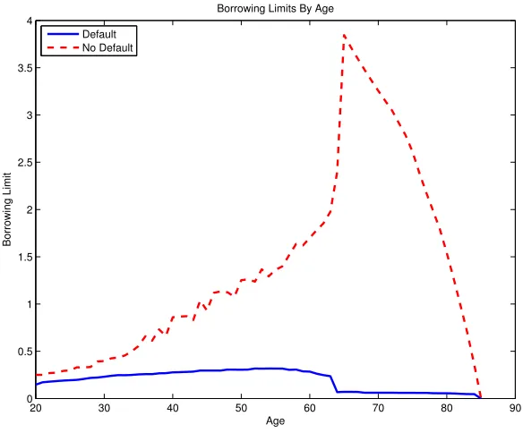
to borrow large amounts while the CD economy does not. One way to see this is to consider borrowing limits in the two economies. While there is no “borrowing limit” in the CD economy, there is a maximum loan size that can be taken out by a household of type s: maxa0q(a0, s)(−a0). Similarly, no household in the ND economy would ever take out a loan

worth more than q( ¯A(s), s)(−A¯(s)) where ¯A(s) is the natural borrowing limit (for types). Figure 1.1 compares these borrowing limits by age (averaging out the other components ofs). As is clear, the maximum loan size in the ND economy is uniformly and typicallymuch

higher than in the CD economy. Because of this, and because households have incentive to use debt, the ND economy is much more indebted. Figure 1.1 also reveals that the elimination of default has a differential effect on the life-cycle profile of borrowing limits. While there are increases for each age, the largest occurs late in life and the smallest when young. Moreover, the shapes are very different with the CD limit tracking the earnings profile and the ND limit sharply increasing until retirement and thereafter sharply decreasing.

(37)

20 30 40 50 60 70 80 90 0

0.5 1 1.5 2 2.5 3 3.5 4

Age

Borrowing Limit

Borrowing Limits By Age Default

No Default

Figure 1.1: Borrowing Limits in the Default and No Default Economies

enter retirement, they face no more uncertainty. This drastically increases the natural limit for all but the unluckiest households.

The borrowing limits in the default economy are shaped by two effects that are quite different from the effects shaping the natural limit. First is that retired households have little incentive to borrow because, by assumption, there is no uncertainty. Consequently, the punishment from default, which to a large extent is exclusion from credit markets, is very low. Because households would readily default, creditors are unwilling to extend much credit. Second is the composition effect caused by a hump-shaped earnings profile.

Conditional on a level of debt and earnings, the incentives to default and repay do not vary much over the life cycle. However, else equal, earnings-rich households are less likely to default. Because average earnings follow a hump shape prior to retirement, so does the average limit.

(38)

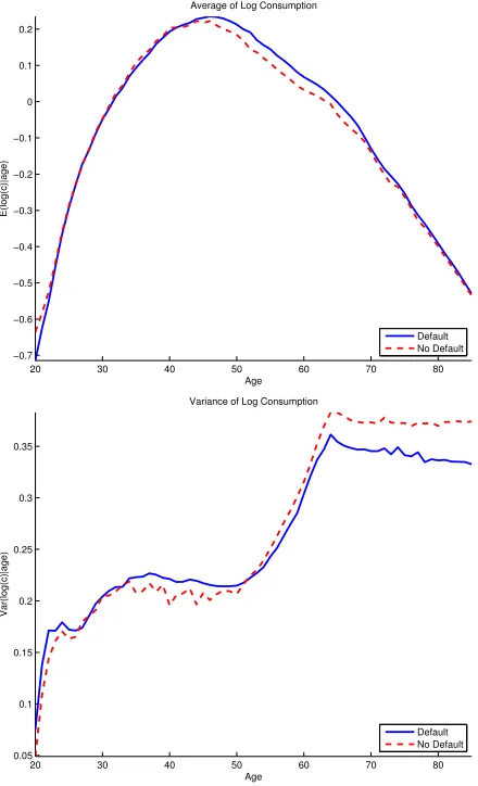
economy until late in life. The interpretation of this is that households in the ND economy borrow heavily when young to smooth consumption while households in the CD economy do not (and cannot) borrow as heavily. In the ND economy, this large amount of debt must eventually be repaid whereas in the CD economy the debt is not as large and can be discharged. This lowers the mean and increases the variance of log consumption later in life in the ND economy. While credit is uniformly better in the ND economy, default does allow households to smooth consumption to some extent. However, the default option has little direct value to young households: to benefit from it, a household must first be indebted.

20 30 40 50 60 70 80 −0.7

−0.6 −0.5 −0.4 −0.3 −0.2 −0.1 0 0.1 0.2

Average of Log Consumption

Age

E(log(c)|age)

Default No Default

20 30 40 50 60 70 80 0.05

0.1 0.15 0.2 0.25 0.3 0.35

Variance of Log Consumption

Age

Var(log(c)|age)

Default No Default

Figure 1.2: Log Consumption in Steady State

(39)

of the CD economy to be indifferent between living in the CD economy and moving to the ND economy.47 This consumption-equivalent variation measure is computed as

ω =



 P

sFˆ(s) R

VN D(0, e, s,0) ˆf(e|s)de P

sFˆ(s) R

VCD(0, e, s,0) ˆf(e|s)de

!1/(1−σ)

−1



 (1.35)

whereVX denotes the value function from theXeconomy. Ifω >0, then eliminating default

is welfare improving. For a more complete picture of the welfare effects, I also report the percentage of the population in favor of the policy change and the welfare gains for various subsets of the population using consumption-equivalent variation.48

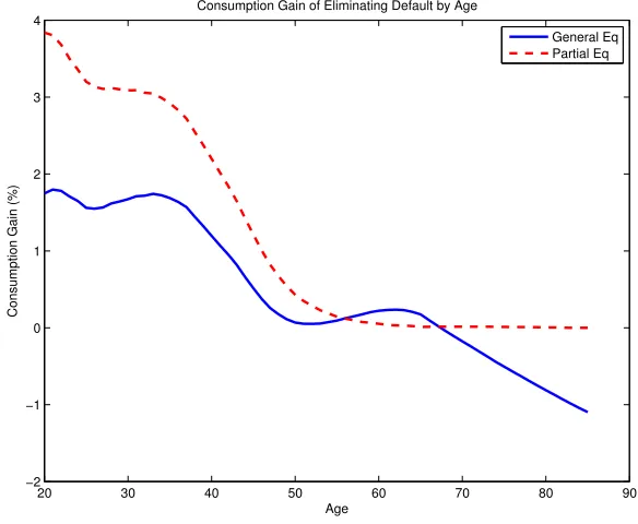
The increased ability to borrow once default is eliminated results in large welfare gains. In general equilibrium, the gain is 1.82% of lifetime consumption. In partial equilibrium, i.e. holding fixed r, w, and ¯qB, it is in fact much larger at 3.94%. Moreover, in partial

equilibrium 100% of the population prefer the move. However, taking general equilibrium effects into account results in substantial disagreement over the policy change: only 56.8% of households now favor it.

To understand who gains and loses from the policy change, it is useful to break out the welfare gains by age both in partial and general equilibrium. This is done in Figure 1.3. In partial equilibrium, the gains begin high for young households, decline monotonically, and approach zero in retirement. The decline is due to diminishing incentives for borrowing: young households have life-cycle reasons to borrow and face uncertainty, middle-aged house-holds have only uncertainty, and retired househouse-holds have neither. Once general equilibrium effects are accounted for, the consumption gains drop sharply for almost all households. This is especially true for young households. Further, now the decline is not monotonic. Be-cause the CD economy has a higher capital-output ratio than the ND economy, households at every age lose labor income from the price changes. At the same time, households with savings gain capital income. Because the primary source of income for most households is

47_{This is the same welfare measure used in}_{Livshits et al.}₍₂₀₀₇_),_{Athreya et al.}₍_2009b_{), and many others.} 48

When calculating welfare gains for different groups, I assume the policy is changed after households have made their default decisions butbefore they have made their savings decisions. Definingω(a, e, s, h) =

((VN D(a, e, s, h)/VCD(a, e, s, h= 0))1/(1−σ)−1),the welfare gain for a subsetIof the population is calculated

as (R

Iω(a, e, s, h)dµ)/µ(I). Here,µis the steady state distribution from the CD economy but with households

who would have defaulted transited to (a, e, s, h) = (0, e, s,0). The population in favor isµ({ω(a, e, s, h)>