Heegaard Floer Invariants and Cabling

University of Pennsylvania

ScholarlyCommons

Publicly Accessible Penn Dissertations

Spring 5-16-2011

Heegaard Floer Invariants and Cabling

Jennifer Hom

University of Pennsylvania, jenhom@math.upenn.edu

Follow this and additional works at:

http://repository.upenn.edu/edissertations

Part of the

Geometry and Topology Commons

This paper is posted at ScholarlyCommons.http://repository.upenn.edu/edissertations/329

For more information, please contactlibraryrepository@pobox.upenn.edu.

Recommended Citation

Hom, Jennifer, "Heegaard Floer Invariants and Cabling" (2011).Publicly Accessible Penn Dissertations. 329.

Heegaard Floer Invariants and Cabling

Abstract

A natural question in knot theory is to ask how certain properties of a knot behave under satellite operations.

We will focus on the satellite operation of cabling, and on Heegaard Floer-theoretic properties. In particular,

we will give a formula for the Ozsvath-Szabo concordance invariant tau of iterated cables of a knot K in terms

of the cabling parameters, tau(K), and a new concordance invariant, epsilon(K). We show that, in many cases,

varepsilon gives better bounds on the 4-ball genus of a knot that tau alone, and discuss further applications of

epsilon. We will also completely classify when the iterated cable of a knot admits a positive L-space surgery.

Degree Type

Dissertation

Degree Name

Doctor of Philosophy (PhD)

Graduate Group

Mathematics

First Advisor

Paul Melvin

Keywords

Heegaard Floer, knot Floer homology, concordance, cables, L-space

Subject Categories

HEEGAARD FLOER INVARIANTS AND CABLING

Jennifer Hom

A Dissertation

in

Mathematics

Presented to the Faculties of the University of Pennsylvania in Partial Fulfillment

of the Requirements for the Degree of Doctor of Philosophy

2011

Paul Melvin, Rachel C. Hale Professor of the Sciences and Mathematics

Supervisor of Dissertation

Jonathan Block, Professor of Mathematics

Graduate Group Chairperson

Dissertation Committee:

James Haglund, Associate Professor of Mathematics

Acknowledgments

I owe an enormous debt of gratitude to my advisor, Paul Melvin. This thesis would not have

been possible without his encouragement, patience, and support.

Nor would this thesis have been possible without the generous support of Robert Ghrist, which

enabled me to spend a year at Berkeley and MSRI, where much of this work was done. While at

MSRI, I had the opportunity to interact with experts in the field, which was enormously helpful.

Among those experts is Matthew Hedden, who laid the foundations on which much of the

work in this thesis is built. His willingness to answer all of my questions began via email before

we had even met, and his responses, then and later, have consistently been very illuminating. I

would also like to thank Peter Ozsv´ath, Dylan Thurston, Robert Lipshitz, Chuck Livingston, Eli

Grigsby, Joan Licata, Rumen Zarev, and Adam Levine for many helpful conversations.

A special thanks goes to Connie Leidy, for first introducing me to what would become the

subject of this thesis, and to Shea Vela-Vick, for his advice and help along the way. I would also

like to thank the PACT crew for creating such a friendly seminar environment, and all of my

colleagues who have invited me to give talks. More generally, a big thank you to everyone who

has shown an interest in my research.

Thanks to Janet Burns, Monica Pallanti, Paula Scarborough, and Robin Toney for helping

the department to run smoothly, to Julius Shaneson and Mark Ward for being on my oral exam

As for my mathematical education prior to Penn, I need to thank my high school calculus

teacher, Mr. Noeth, for taking, sticking, and d-ing it, and for flinging it over there. I would also

like to finally thank, rather than blame, Linda Chen for her abstract algebra class that first caused

me to seriously consider a career in math.

To all of my friends, thank you for the encouragement and distraction, or rather, in the case

of Colin Diemer and Dave Favero, the (joking, I think) discouragement and distraction. Thanks

also to my officemate Tim DeVries, for the years of commiseration. Other notable distractions

include Quizo, Settlers of Catan, Rock Band, and all of the people who made those activities so

enjoyable. I’d also like to thank all of my friends, both human and animal, who got to experience

living with me, and my AB girls, for many, many years of friendship.

I wouldn’t be where I am today if it weren’t for my parents, and the myriad of educational

opportunities that they provided for me. Thanks also to Delia and Eugene, and especially to my

niece Tae, who knows that you can’t really draw a line, and that the statement “A tautology is a

tautology” is meta.

Finally, I would like to thank Chris, for putting up with me for the past five years and hopefully

ABSTRACT

HEEGAARD FLOER INVARIANTS AND CABLING

Jennifer Hom

Paul Melvin, Advisor

A natural question in knot theory is to ask how certain properties of a knot behave under

satellite operations. We will focus on the satellite operation of cabling, and on Heegaard

Floer-theoretic properties. In particular, we will give a formula for the Ozsv´ath-Szab´o concordance

invariant τ of iterated cables of a knotK in terms of the cabling parameters, τ(K), and a new

concordance invariant, ε(K). We show that, in many cases, ε gives better bounds on the 4-ball

genus of a knot thatτalone, and discuss further applications ofε. We will also completely classify

Contents

1 Introduction 1

2 A quick trip through bordered Heegaard Floer homology 6

2.1 Algebraic preliminaries . . . 6

2.2 Bordered Heegaard Floer homology . . . 8

2.3 The knot Floer complex . . . 21

2.4 From the knot Floer complex to the bordered invariant . . . 26

3 Definition and properties of ε(K) 31 4 Computation ofτ for (p, pn+ 1)-cables 40 4.1 The caseε(K) = 1 . . . 41

4.2 The caseε(K) =−1 . . . 49

4.3 The caseε(K) = 0 . . . 50

5 Computation ofτ for general (p, q)-cables 53

6 Computation ofε(Kp,pn+1)when ε(K) = 1 56

7 Computation ofε for (p, q)-cables 61

9 Cabling and L-space Knots 66

List of Figures

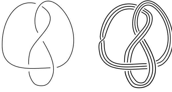
1.1 The figure 8 knot, and its (3,1)-cable . . . 1

2.1 Pointed matched circles . . . 10

2.2 The idempotents and algebra elements . . . 11

2.3 A decorated source . . . 14

2.4 Bordered Heegaard diagrams to computeCF Dd for a solid torus . . . 16

2.5 Bordered Heegaard diagrams to computeCF Ad for a solid torus . . . 19

2.6 CF K∞ _{andCF Dd for different knots and their framed complements . . . . 30}

3.1 CF K∞_{(K) for different knotsK . . . . 36}

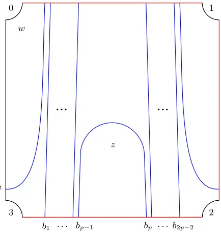
4.1 The bordered Heegaard diagramH(p,1) . . . 42

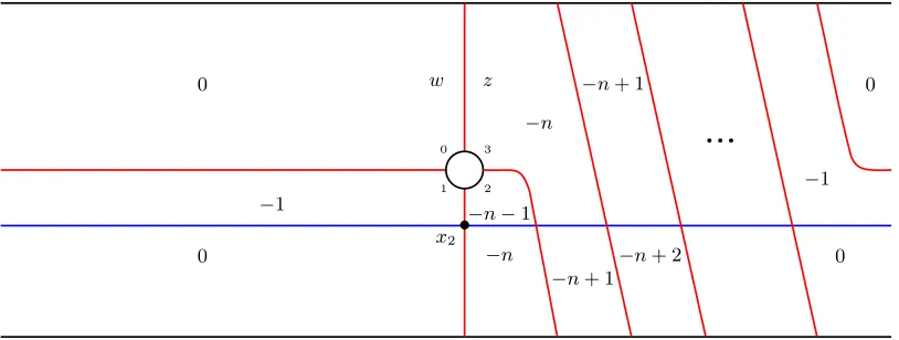
4.2 Winding region for a knot complement . . . 46

4.3 Winding region for a bordered knot complement . . . 46

4.4 Stabilized bordered Heegaard diagramH(p,1) . . . 47

4.5 The periodic domainPµ inH(p,1). . . 48

4.6 The periodic domainPλ inH(p,1) . . . 52

Chapter 1

Introduction

In this thesis, we address the question of how certain properties of knots behave under the satellite

operation of cabling. The (p, q)-cable of a knotK, denotedKp,q, is the satellite knot with pattern

the (p, q)-torus knotTp,q(wherepindicates the longitudinal winding andqindicates the meridional

winding) and companionK. We will assume throughout thatp >1. (This assumption does not

cause any loss of generality, since K−p,−q = rKp,q, where rKp,q denotes Kp,q with the opposite

orientation, and sinceK1,q=K.)

It is well-known that the Alexander polynomial of the (p, q)-cable of a knotK is completely

determined byp,q, and the Alexander polynomial ofK, ∆K(t), in the following manner:

∆Kp,q(t) = ∆K(t

p_)·∆ Tp,q(t),

where

∆Tp,q(t) =

(tpq_−1)(t−1)

(tp_−1)(tq₋₁₎.

In this thesis, we focus on the behavior of the Ozsv´ath-Szab´o concordance invariant τ under

cabling.

Two knots K0, K1 ⊂S3 are called concordant, denoted K0 ∼ K1, if there exists a smooth,

properly embedded cylinder in S3_{×[0,1] such that one end of the cylinder is K}

0× {0} and the

other is K1× {1}. This gives us an equivalence relation on the set of knots. A knotK is called

slice ifK is concordant to the unknot. The set {K}/ ∼forms the concordance group C, where

the operation is induced by connected sum. The class of slice knots is the identity element, and

the inverse of [K] is [−K], where−K denotes the reverse of the mirror image ofK. If we loosen

the conditions and only require that the cylinder be locally flat, rather than smooth, we obtain

thetopological concordance group.

To a knotK ⊂S3_{, Ozsv´ath and Szab´o [11], and independently Rasmussen [19], associate a}

Z_⊕Z_{-filtered chain complexCF K}∞_{(K), whose doubly filtered chain homotopy type is an invariant}

ofK. Looking at just one of the filtrations (i.e., taking the degree zero summand of the associated

graded object with respect to the other filtration) yields the Z_{-filtered chain complexCF K}\_(K),

and associated to this chain complex is theZ_{-valued smooth concordance invariantτ(K); see [9].}

In [9], Ozsv´ath and Szab´o show that the concordance invariantτ has the following properties:

1. τ:C →Z_{is a surjective homomorphism.}

2. |τ(K)| ≤g4(K), whereg4(K) denotes the smooth 4-ball genus ofK.

We completely describe the behavior of τ under cabling, generalizing work of Hedden [2], Van

Cott [20], and Petkova [18]. As one might expect, τ(Kp,q) is closely related toτ(Tp,q). However,

it depends on strictly more than just τ(K), p, andq; we also need to know the value ofε(K), a

new{−1,0,1}-valued concordance invariant associated to the knot Floer complexCF K∞(K).

Theorem 1. The behavior of τ(Kp,q) is completely determined by p, q, τ(K), and ε(K). In particular,

1. Ifε(K) = 0, thenτ(K) = 0 andτ(Kp,q) =τ(Tp,q) =

      

(p−1)(q+1)

2 ifq <0

(p−1)(q−1)

2 ifq >0.

2. Ifε(K)6= 0, then

τ(Kp,q) =pτ(K) +

(p−1)(q−ε(K))

2 .

One consequence of Theorems 1 and 2 is that the only additional concordance information about

Kcoming fromτof iterated cables ofKis the invariantε. Conversely, knowingτof just two cables

ofK, one positive and one negative, is sufficient to determineε(K). In particular, knowing

infor-mation about the Z_{-filtered chain complexCF K}\_{(Kp,q), namely τ(Kp,q), can tell us information}

about theZ_⊕Z_{-filtered chain complexCF K}∞_{(K), i.e.,ε(K).}

Sinceτ(Kp,q) depends on both τ(K) andε(K), we would also like to know the behavior ofε

under cabling in order to compute τ of iterated cables.

Theorem 2. The invariant εbehaves in the following manner under cabling:

1. Ifε(K) = 0, thenε(Kp,q) =ε(Tp,q) =

              

−1 if q <−1

0 if |q|= 1

1 if q >1.

2. Ifε(K)6= 0, thenε(Kp,q) =ε(K)for allpandq.

We see thatτ(Kp,q) depends on strictly more than justτ(K), so it is natural to ask if there exist

knots K and K′ _{with τ(K) = τ(K}′_{) but τ(K}

p,q) 6= τ(Kp,q′ ). We answer this question in the

Corollary 3. For any integern, there exists knots K andK′ _{with τ(K) =τ(K}′_{) =n, such that} τ(Kp,q)6=τ(Kp,q′ ), for allpandq,p6= 1.

Recall that the absolute value ofτ(K) gives a lower bound on the 4-ball genus of a knot; that is,

g4(K)≥ |τ(K)|. By looking at bothτ and ε, we can give stronger bounds in many cases. The

following corollary was suggested to me by Livingston:

Corollary 4 (Livingston). If ε(K)6= sgnτ(K), theng4(K)≥ |τ(K)|+ 1.

If two knots are concordant, it follows that their cables are also concordant. Thus, it follows

from Therorem 1 thatεis a concordance invariant. We also prove the following properties about

ε:

• IfK is slice, thenε(K) = 0.

• ε(−K) =−ε(K).

• Ifε(K) = 0, then τ(K) = 0.

• There exist knotsK with τ(K) = 0 butε(K)6= 0; that is, ε(K) isstrictly stronger than

τ(K) at obstructing sliceness.

• Letg(K) denote the genus ofK. If|τ(K)|=g(K), thenε(K) = sgnτ(K).

• IfKishomologically thin(meaningHF K\(K) is supported on a single diagonal with respect

to its bigrading), thenε(K) = sgnτ(K).

• Ifε(K) =ε(K′_{), thenε(K#K}′_{) =ε(K) =ε(K}′_{). Ifε(K) = 0, thenε(K#K}′_{) =ε(K}′_).

Moreover, the invariant εcan be used to define a new concordance homomorphism, as discussed

in [4].

In the latter part of this thesis, we will consider a special kind of 3-manifold, called anL-space,

and knots on which some positive integral surgery yields an L-space. Such a knot is called an

Letg(K) denote the Seifert genus ofK. In Theorem 1.10 of [2], Hedden proves that ifK is

anL-space knot and q/p≥2g(K)−1, thenKp,q is anL-space knot. We will prove the converse:

Theorem 5. The (p, q)-cable of a knotK⊂S3 _{is anL-space knot if and only ifKis anL-space} knot and q/p≥2g(K)−1.

Thus, we see that whether or not the cable of Kis anL-space knot depends only on the cabling

parameters, and whether or notKis anL-space knot. The proof of this theorem relies on classical

Chapter 2

A quick trip through bordered

Heegaard Floer homology

We begin with a few algebraic preliminaries, before proceding to a brief overview of bordered

Heegaard Floer homology and knot Floer homology.

2.1

Algebraic preliminaries

For the reader unfamiliar with the algebraic structures involved in bordered Heegaard Floer

ho-mology, such as A∞-modules, the Type D structures of [7], and the “box” tensor product, we

recount the definitions below. For a more detailed description, we refer the reader to [7, Section

2].

LetAbe a unital graded algebra overF₌Z_/2Z_{with an orthogonal basis{ιi}for the subalgebra}

of idempotents, I ⊂ A, such thatPιi = 1 ∈ A. In what follows, all of the tensor products are

A(right unital)A∞-module is anF-vector spaceM equipped with a rightI-action such that

M =M

i M ιi,

and a family of maps

mi:M ⊗ A⊗i−1→M

satisfying the A∞conditions

0 =

n−1 X

i=1

mn−i+1(mi(x⊗a1⊗. . .⊗ai−1)⊗. . .⊗an−1)

+

n−2 X

i=1

mn−1(x⊗a1⊗. . .⊗aiai+1⊗. . . an−1)

and the unital conditions

m2(x,1) =x

mi(x, . . . ,1, . . .) = 0, i >2.

We say thatM isbounded if there exists an integernsuch thatmi= 0 for alli > n.

AType D structure overAis anF_{-vector spaceN equipped with a left I-action such that}

N=M

i ιiN,

and a map

δ1:N → A ⊗N

satisfying the TypeD condition

(µ⊗I_N)◦(I_{A⊗δ1)◦δ1= 0,}

where µ:A ⊗ A → Adenotes the multiplication onA.

On the TypeD structureN, we define maps

inductively by

δ0=IN

δi= (IA⊗i−1⊗δ1)◦δi−1.

We say thatN isbounded if there exists an integernsuch thatδi= 0 for alli > n.

Thebox tensor product M ⊠N is theF_{-vector space}

M⊗IN,

endowed with the differential

∂⊠(x⊗y) =

∞ X

k=0

(mk+1⊗IN)(x⊗δk(y)).

If at least one ofM orN is bounded, then the above sum is guaranteed to be finite.

The above definitions can be suitably modified if one would like to work over a differential

graded algebra instead of merely a graded algebra; see [7, Section 2] or [6, Section 2.1].

2.2

Bordered Heegaard Floer homology

We assume the reader is familiar with Heegaard Floer homology for closed 3-manifolds, and with

the filtration induced on this invariant by a knot K in the 3-manifold. See, for example, the

expository overview [14]. We begin with an overview of the invariants associated to 3-manifolds

with parameterized boundary, as defined by Lipshitz, Ozsv´ath and Thurston in [7]. Let Y be

a closed 3-manifold. Decompose Y along a closed surface F into pieces Y1 and Y2 such that

∂Y1 = −∂Y2 = F. In particular, this gives us an orientation preserving diffeomorphism from

F to ∂Y1, and an orientation reversing diffeomorphism from F to ∂Y2. A 3-manifold with a

diffeomorphism (up to isotopy) from a standard surface to its boundary is called a bordered 3

-manifold, and we call this isotopy class of diffeomorphisms a marking of the boundary. To the

[

CF A(Y1), which will be a rightA∞-module over the algebraA(F), while toY2, we associate the

invariant, \CF D(Y2), which will be a Type D structure. To a knotK in Y1, we may associate

eitherCF A[(Y1, K), a filteredA∞-module, orCF A−(Y1, K), anA∞-module over the ground ring F_[U].

The pairing theorems of [7, Theorems 1.3 and 10.12] state that there exists a quasi-isomorphism

betweenCFd(Y) and the box tensor product of CF A[(Y1) andCF D\(Y2):

d

CF(Y)≃CF A[(Y1)⊠CF D\(Y2).

We may also consider the case where we have a knotK1⊂Y1, in which case we have the following

quasi-isomorphism ofZ_{-filtered chain complexes:}

\

CF K(Y, K)≃CF A[(Y1, K1)⊠CF D\(Y2),

and the following quasi-isomorphism ofF_[U]-modules:

CF K−(Y, K)≃CF A−(Y1, K1)⊠CF D\(Y2).

Note that the information contained in the Z_{-filtered chain complex CF K}\_{(Y, K) is equivalent}

to that in the F_{[U]-moduleCF K}−_{(Y, K). Similar pairing theorems hold when we have a knot}

K2⊂Y2.

In this thesis, we will use these tools to study cabling. Thus, we will restrict ourselves to the

case whereF is a torus. To use the bordered Heegaard Floer package to study the (p, pn+ 1)-cable

of a knot K, we will letY1 be a solid torus equipped with a (p,1)-torus knot, and letY2 be the

knot complement S3_{−nbd K with framing n; that is, the marking specifies a meridian of the}

knot and an-framed longitude.

We will now describe the algebraA(F), the modulesCF A[(Y1) and CF D\(Y2), and the box

tensor product, all in the case of F =T2_{. WhenF is a torus, A(F) is merely a graded algebra,}

while when g(F)≥2, it is adifferential graded algebra. At the end of this section, we note the

To specify the identification ofT2 _with∂Y

1 and−∂Y2, we need to identify a meridian and a

longitude of the torus. One way to do this is to specify a handle-decomposition for the surface;

that is, a disk with two 1-handles attached such that the resulting boundary is connected and can

be capped off with a disk. For technical reasons, we also place a basepoint somewhere along the

boundary of the disk.

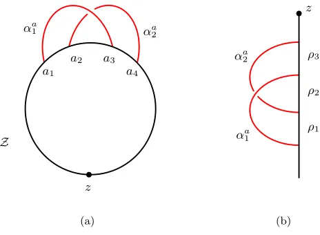
Schematically, we can represent this information by apointed matched circle, which we think

of as the boundary of the disk with markings at the feet of the 1-handles. In this case, the pointed

matched circle Z consists of a circle with five marked points: a1,a2, a3, a4, andz, in that order

as we traverse the circle in the clockwise direction, where the arcαa

1 has endpoints at a1and a3,

and the arcαa

2 has endpoints ata2 anda4.

z

Z

αa

1 _αa

2

a1

a2 a3

a4 (a) z αa 1 αa 2 ρ1 ρ2 ρ3 (b)

Figure 2.1: Above left, the pointed matched circle for the surface T2_{. Above right, the same}

pointed matched circle cut open at z.

To the surfaceT2_{parametrized by the pointed matched circleZ, we associate a graded algebra,}

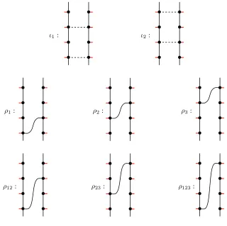
A(T2_{). The algebraA(T}2_{) is generated overFby the two idempotents}

ι1 and ι2,

and the six “Reeb” elements

These algebra elements may be understood pictorially, as in Figure 2.2, where multiplication is

understood to correspond to concatenation.

ι1: ι2:

ρ1: ρ2: ρ3:

ρ12: ρ23: ρ123:

Figure 2.2: The idempotents and algebra elements.

The idempotents correspond to αa

1 and αa2, respectively. We will often need to consider the

ring of idempotents,

I=F_{hι1i ⊕}F_hι2i.

We have the following compatibility conditions with the idempotents:

ρ1=ι1ρ1=ρ1ι2 ρ2=ι2ρ2=ρ2ι1 ρ3=ι1ρ3=ρ3ι2

ρ12=ι1ρ12=ρ12ι1 ρ23=ι2ρ23=ρ23ι2 ρ123=ι1ρ123=ρ123ι2,

and the following non-zero products:

We will letρ1refer to the arc ofZ − {z}betweena1anda2,ρ2the arc betweena2anda3, andρ3

the arc betweena3anda4. Similarly,ρ12,ρ23andρ123will refer to the appropriate concatenations.

This completes the description of the algebraA(T2_{). See Section 3 of [7] for the full description}

of the algebra in the general case.

A bordered Heegaard diagram for a 3-manifold Y with ∂Y = T2 _{is a tuple (Σ,α}c_,αa_{,β, z)}

consisting of the following:

• a compact, oriented surface Σ of genusg with a single boundary,∂Σ

• a (g−1)-tuple of pairwise disjoint circlesαc= (αc

1, . . . , αcg−1) in the interior of Σ

• a pair of disjoint arcsαa = (αa

1, αa2) in Σ\αc with endpoints on∂Σ

• ag-tuple of pairwise disjoint circlesβ= (β1, . . . , βg) in the interior of Σ

• a basepointzonZ\∂αa

Letα denoteαc∪αa. We further require that all intersections be transverse and that Σ\αand

Σ\βare connected. The data{∂Σ, z, ∂αa

1, ∂αa2} describes a pointed matched circle.

For bordered Heegaard diagrams, there are two types of periodic domains, and hence two

notions of admissibility. Consider closed domains P in Σ whose interiors consist of linear

combi-nations of connected components in Σ\(αa,αc,β). We callP aperiodic domain if∂P consists of

a collection of α-arcs, α-circles, β-circles, and arcs in ∂Σ, with z /∈ ∂P. We call P a provincial

periodic domain if∂P consists of a collection of full α-circles and β-circles, withz /∈∂P. Notice

that this implies thatP is not adjacent to∂Σ.

We say a bordered Heegaard diagram is provincially admissible if every provincial periodic

domain has both positive and negative multiplicities. A bordered Heegaard diagram isadmissible

if every periodic domain has both positive and negative multiplicities. Provincial admissibility

is sufficient for the bordered invariants to be well-defined, and admissibility is sufficient for the

To construct a 3-manifold with parameterized boundary, Y, from the data (Σ,αc,αa,β, z) ,

we attach 2-handles to Σ×[0,1] alongαc× {0}andβ× {1}. The parametrization of the boundary

ofY is given by the identification of{∂Σ, z, ∂αa

1, ∂αa2} × {0}with the pointed matched circleZ.

LetHbe a bordered Heegaard diagram forY. We will now describe the invariants\CF D(H)

and CF A[(H). The set of generators, S_{(H), are unorderedg-tuples of intersection points of α}

-andβ-curves such that

• eachβ-circle is occupied exactly once

• eachα-circle is occupied exactly once

• eachα-arc is occupied at most once.

In the case we are considering, where ∂Y =T2_{, notice that these conditions imply that exactly}

one of the α-arcs is occupied.

We now define the TypeDstructureCF D\(H). We identify{∂Σ, z, ∂αa

1, ∂αa2}with−Z. Let

\

CF D(H), or simplyCF D\, denote theF_{-vector space generated by}S_{(H), with the leftI-action}

onx∈S_{(H) defined to be}

ι1x=       

x ifxdoesnot occupy the arcαa

1

0 otherwise

ι2x=       

x ifxdoesnot occupy the arcαa

2

0 otherwise.

We will define maps

δ1:CF D\→ A ⊗CF D\

by counting certain pseudo-holomorphic curves. Note that the above tensor product is over the

ring of idempotents,I, as are the rest of the tensor products in this section. Let Σ denote Int Σ.

Define a decorated source S⊲ _{to be a topological type of smooth surfaceS with boundary and a}

• a labeling of each puncture by one of−, +, ore

• a labeling of eachepuncture ofS by a Reeb chordρ.

Consider the 4-manifold Σ×[0,1]×R_{, with the following projection maps:}

πΣ: Σ×[0,1]×R→Σ

πD: Σ×[0,1]×R→[0,1]×R

πI : Σ×[0,1]×R→[0,1]

πR: Σ×[0,1]×R→R.

Let Σe denote Σ with its puncture filled in. Similarly, letSe denoteS with its epunctures filled

in.

− +

ρ1 ρ2

Figure 2.3: A decorated source,S⊲_.

We are interested in proper maps

u: (S, ∂S)→ Σ×[0,1]×R_{,(α× {1} ×}R_{)∪(β× {0} ×}R₎

such that

• The mapπD◦uis ag-fold branched cover.

• At each−-punctureqofS, limz→q(πR◦u)(z) =−∞.

• At each +-punctureqofS, limz→q(πR◦u)(z) = +∞.

• πΣ◦udoes not cover the region of Σ adjacent to z.

• The mapuextends to a proper mapue:Se→Σe×[0,1]×R.

• For each t ∈ R _{and each i = 1, . . . , g, there is exactly one point in u}−1_(β

i × {0} × {t}).

Similarly, for eacht∈ R_{and each i= 1, . . . , g−1, there is exactly one point in u}−1_(αc i ×

{0} × {t}).

We also require the maputo beJ-holomorphic and of finite energy in the appropriate sense. See

Section 5 of [7].

The map πR◦ue gives an ordering on the e punctures, and their respective labels; this is

induced by theR_{-coordinate of their images. We denote the resulting sequence of Reeb chords by}

− →_{ρ = (ρ}

i1, . . . , ρin).

We let MB_(x,y,−→_{ρ) denote a certain reduced moduli space. Roughly, this moduli space}

consists of curves from a decorated source S⊲ with asymptotics corresponding to −→ρ and in the

homology classB∈π2(x,y), whereπ2(x,y) is the set of homology classes of curves connectingx

to y. The index ind(B,−→ρ) is equal to the expected dimension of MB_(x,y,−→_{ρ)plus one.}

The mapδ1 is defined as:

δ1(x) := X

y∈S(H)

X

B∈π2(x,y) {−→ρ|ind(B,−→ρ)=1}

# MB_(x,y,−→

ρ)ρi1·. . .·ρin⊗y,

where # MB_(x,y,−→_{ρ) is the number of points, modulo two, in the zero-dimensional moduli}

spaceMB_(x,y,−→_{ρ). Provincial admissibility implies that the sum is well-defined.}

As in the theory for closed 3-manifolds, there is a combinatorial formula to compute the index

of a map, in terms of the Euler measure and local multiplicities of the associated domain on Σ

(that is, the image ofπΣ◦u), and the manner in which the domain abuts∂Σ. See Definition 5.46

z

αa

1

αa

2

ρ1 ρ2

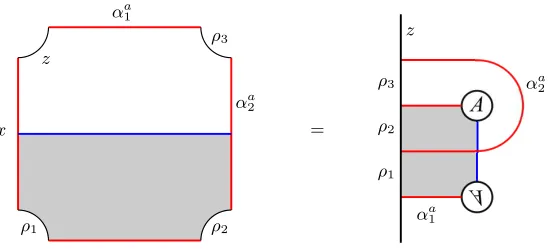
ρ3 x = ρ1 ρ2 ρ3 z αa 2 αa 1

(a) Two different ways of viewing the Heegaard diagram H0. The

shaded region contributes to the mapδ1(x) =ρ12x.

z

ρ1 ρ2

ρ3

x

y1 . . . yn

(b) The Heegaard diagramH_n.

z

ρ1 ρ2

ρ3

x

y1 . . . yn

(c) The Heegaard diagramH_−n.

Figure 2.4: Three bordered Heegaard diagrams for the solid torus, labeled to compute\CF D, with

different parametrizations of the boundary. In 2.4(a), we show two equivalent ways of drawing

the Heegaard surface: first, as a square with opposite sides identified, and second, as a disk with

a 1-handle attached.

Example 2.1. The invariant \CF D(H0) associated to the bordered Heegaard diagram in Figure 2.4(a) has a single generator xin the idempotentι1 and the map

δ1:x7→ρ12x.

the maps

δ1:x7→ρ123y1

δ1:yi7→ρ23yi+1, 1≤i≤n−1

δ1:yn 7→ρ2x.

Example 2.3. The invariantCF D\(H−n)associated to the bordered Heegaard diagram in Figure 2.4(b) has one generatorxin the idempotentι1,ngenerators y1, . . . , yn in the idempotentι2 and

the maps

δ1:x7→ρ1y1

δ1:yi7→ρ23yi−1, 2≤i≤n

δ1:x7→ρ3yn.

To complete the definition of the TypeD structure onCF D\, we define the maps

δk:CF D\→(A⊗k⊗\CF D)

inductively by

δ0=I_{\CF D}

δi= (IA⊗i−1⊗δ1)◦δi−1.

Recall that \CF Disbounded if there exists an integerN such that δi = 0 for alli > N. Lemma

6.5 of [7] tells us that ifHis admissible, thenCF D\(H) is bounded.

We now defineCF A[. We identify{∂Σ, z, ∂αa

1, ∂αa2} withZ. As anF-vector space,CF A[ is

generated byS_{(H), with the rightI-action defined to be}

xι1=       

x ifxoccupies the arcαa1

0 otherwise

xι2=       

x ifxoccupies the arcαa

2

TheA∞-structure onCF A[ is defined by counting certain pseudoholomorphic curves, giving maps

mj+1:CF A[ ⊗ A⊗j→CF A,[

defined to be

mj+1(x, ρi1, . . . , ρij) =

X

y∈S(H) X

B∈π2(x,y) ind(B,−→ρ)=1

# MB(x,y,−→ρ)y

m2(x,1) =x

mj+1(x, . . . ,1, . . .) = 0, j >1.

As in the case of \CF D, provincial admissibility of the Heegaard diagram guarantees that the

above sum is well-defined. Recall that CF A[ is bounded if there exists an integer N such that

mj= 0 for allj > N. IfHis admissible, thenCF A[ is bounded.

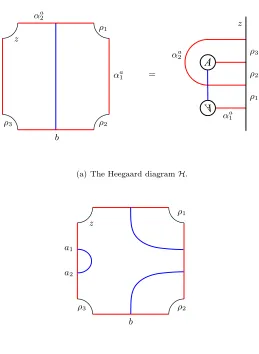
Example 2.4. The invariant CF A[(H) associated to the bordered Heegaard diagram in Figure 2.5(a) has a single generator bin the idempotent ι2, with the algebra relations

m3+i(b, ρ2,

i

z }| {

ρ12, . . . , ρ12, ρ1) =b, i≥0.

Example 2.5. The invariant CF A[(H′_{) associated to the bordered Heegaard diagram in Figure} 2.5(b) has two generatorsa1anda2in the idempotentι1and a single generatorbin the idempotent

ι2, with the algebra relations

m1(a1) =a2

m2(a1, ρ12) =a2

m2(a1, ρ1) =b

m2(b, ρ2) =a2

The tensor productCF A[ ⊠CF D\ is theF_{-vector space}

[

z αa

2

αa

1

ρ3 ρ2

ρ1

b

=

ρ3

ρ2

ρ1

z

αa

2

αa

1

(a) The Heegaard diagramH_.

z

ρ3 ρ2

ρ1

b a2

a1

(b) The admissible Heegaard diagramH′_.

Figure 2.5: A bordered Heegaard diagram for the framed solid torus, labeled to compute the

invariant CF A[. In 2.5(a), we show the Heegaard surface first as a square with opposite sides

identified, and second as disk with a 1-handle attached. In 2.5(b), we have isotoped the β-circle

so that the diagram is admissible.

equipped with the differential

∂⊠(x⊗y) =

∞ X

k=0

(mk+1⊗I_{\CF D})(x⊗δk(y)).

If at least one ofCF A[ and\CF Dis bounded, then the above sum is guaranteed to be finite.

calculations. Defineρ∅ to beι1+ι2. Then we can rewriteδ1 as

δ1= X

i

ρi⊗Di,

where the sum is taken overi∈ {∅,1,2,3,12,23,123}, and theDi are coefficient maps

Di:CF D\→CF D.\

The tensor productCF A[ ⊠CF D\is still theF_{-vector space}

[

CF A⊗I\CF D,

with the differential now given by

∂⊠(x⊗y) =Xmk+1(x, ρi1, . . . , ρik)Dik◦. . .◦Di1(y),

where the sum is taken over allk-element sequencesi1, . . . , ik (including the empty sequence when

k= 0) of elements in{∅,1,2,3,12,23,123}.

Example 2.6. Using Examples 2.2 and 2.5 above, we compute the tensor product CF A[(H′_)⊠ \

CF D(Hn)≃CFd(Ln,1). The generators in the tensor product are

a1x, a2x, by1, . . . , byn,

with the differential

∂(a1x) =a2x.

Example 2.7. Using Examples 2.1 and 2.5 above, we compute the tensor product CF A[(H′_)⊠ \

CF D(H0)≃dCF(S1×S2). Note that the only nontrivial coefficient map onCF D\(H0)is

D12(x) =x.

The generators in the tensor product are a1xanda2x, with trivial differential since

We conclude this section by highlighting a few of the differences that occur when∂Y has genus

≥2.

A bordered Heegaard diagram for a 3-manifoldY with parameterized boundaryF of genusk

consists of a punctured surface Σ of genus g, ag-tuple of β-circles, a (g−k)-tuple of α-circles,

a 2k-tuple of α-arcs, and a basepoint z on ∂Σ, such that Σ\α and Σ\β are connected (where

α denotes the collection ofα-arcs and -circles, and βdenotes the collection of β-circles). Notice

that when g(F)≥2, there is a not a unique parametrization (i.e., handle-decomposition) of the

diffeomorphism type of F, hence there is not a unique algebra associated to the diffeomorphism

type of the surfaceF. In other words, for different pointed matched circle describing a surface of

genus g(F), we get a different algebra.

Furthermore, while in the case of torus boundary, A(T2_{) is a simply a graded algebra, the}

algebra associated to a parameterized surface of genus 2 or higher is a differential graded algebra.

See Section 3 of [7] for details.

In the case of torus boundary, each generatorxoccupies exactly oneα-arc, hence for a mapu, we have at most one Reeb chord occurring at any given time (i.e., theR_{-coordinate of its image).}

Thus, the mapuallows us to consider a sequence of Reeb chords. In the general case, it is possible

for multiple Reeb chords to occur at the same time, souinduces a sequence ofsetsof Reeb chords

instead. See Section 5 of [7] for a complete description, or Section 5 of Zarev [21] for a description

of the analogous construction in the bordered sutured case.

2.3

The knot Floer complex

We now review some basic facts about the various flavors of the knot Floer complex, defined by

Ozsv´ath and Szab´o in [11] and independently by Rasmussen in [19]. For an expository overview of

these invariants, we again refer the reader to [14]. We specify a knotK⊂S3_{by a doubly pointed}

the α- andβ-circles. The chain complex CF K−_{(K) is freely generated over F[U] by the set of}

g-tuples of intersection points between the α- andβ-circles, where each α- and each β-circle are

used exactly once, andg is the genus of the surface Σ. The differential is defined as

∂x:= X

y∈S(H) X

φ∈π2(x,y) ind(φ)=1

#M(c φ)Unw(φ)_·y.

This complex has a homological Z_{-grading, called the Maslov grading M, as well as a} Z

-filtration, called theAlexander filtration A. The relative Maslov and Alexander gradings are defined

as

M(x)−M(y) = ind(φ)−2nw(φ) and A(x)−A(y) =nz(φ)−nw(φ),

for φ ∈ π2(x,y). The differential, ∂, decreases the Maslov grading by one, and respects the

Alexander filtration; that is,

M(∂x) =M(x)−1 and A(∂x)≤A(x).

Multiplication by U shifts the Maslov grading and respects the Alexander filtration as follows:

M(U·x) =M(x)−2 and A(U·x) =A(x)−1.

Setting U = 0, we obtain the filtered chain complex CF K\(K) =CF K−(K)/(U = 0). The total

homology of CF K\(K) is isomorphic toHFd(S3)∼=F_{. The normalization for the Maslov grading}

is chosen so that the generator forHFd(S3_{) lies in Maslov grading zero. We denote the homology}

of the associated graded object of CF K\(K) by

\

HF K(K) =M

s \ HF K(K, s),

where s indicates the Alexander grading induced by the filtration. Similarly, we denote the

homology of the associated graded object ofCF K−_{(K) by}

HF K−(K) =M

s

We normalize the Alexander grading so that

min{s|HF K\(K, s)6= 0}=−max{s|HF K\(K, s)6= 0}.

Equivalently, we can define the absolute Alexander grading of a generatorxto be

A(x) = 1

2hc1(s(x)),[Fb]i,

where Fb is a Seifert surface for K capped off in the 0-surgery,s x)∈Spinc(S3 0(K)

denotes the

Spinc structure overS3

0(K) associated to the generatorxby the basepointswandz, andc1(s(x))

is the relative first Chern class ofs₍x); see [11, Section 3]. At times, we will consider the closely related complex

CF K∞(K) :=CF K−(K)⊗_F[U]F[U, U−1],

which is naturally a Z_⊕Z_{-filtered chain complex, with one filtration induced by the}

Alexan-der filtration and the other by −(U-exponent). It is often convenient to view CF K∞(K) and

CF K−(K) graphically in the (i, j)-plane, suppressing the homological grading from the picture,

where the i-coordinate corresponds to−(U-exponent), and the j-coordinate corresponds to the

Alexander grading. An element of the formUi_{·xis plotted at the coordinate (−i, A(U}i_{·x)), or}

equivalently, (−i, A(x)−i). In particular, the complexCF K−_{(K) is contained in the part of the}

(i, j)-plane withi≤0, and a generatorxofCF K−_{(K) has coordinates (0, A(x)).}

We may denote the differential by arrows which will necessarily point non-strictly downwards

and to the left. We say that (i′_{, j}′_{)≤(i, j) if i}′ _{≤i andj}′ _{≤j. Given S⊂}Z_⊕Z_{, we let C{S}}

denote the set of elements inCF K∞(K) whose (i, j)-coordinates are in S. IfS has the property

that (i, j)∈S implies that (i′, j′)∈Sfor all (i′, j′)≤(i, j), thenC{S}inherits the structure of a

subcomplex. Similarly, for appropriateS,C{S}may inherit the structure of a quotient complex,

or of a subquotient complex. For example,CF K\(K) is the subquotient complexC{i= 0}.

The integer-valued smooth concordance invariantτ(K) is defined in [9] to be

where ιis the natural inclusion of chain complexes. Alternatively,τ(K) may be defined in terms

of theU-action onHF K−_{(K), as in [17, Appendix A]:}

τ(K) =−max{s| ∃[x]∈HF K−(K, s) such that∀ d≥0, Ud[x]6= 0}.

Recall that the complex CF K∞(K) is doubly filtered, by the Alexander filtration, and by

powers ofU. Taking the degree 0 part of the associated graded object with respect to the Alexander

filtration, we define the horizontal complex,

Chorz_{:=C{j= 0},}

equipped with a differential,∂horz_{. Graphically, this can be viewed as the subquotient complex of}

CF K∞_{(K) consisting of elements withj-coordinate equal to zero, with the induced differential}

consisting of horizontal arrows pointing non-strictly to the left. The horizontal complex inherits the

structure of a Z_{-filtered chain complex, with the filtration induced by−(U-exponent). Similarly,}

we may consider the degree 0 part of the associated graded object with respect to the filtration

by powers of U, and define thevertical complex,

Cvert:=C{i= 0},

equipped with a differential, ∂vert_{. Note that this is equivalent toCF K}−_{(K)/(U ·CF K}−_(K)).

In the vertical complex, the induced differential may be graphically depicted as vertical arrows

pointing non-strictly downwards. The vertical complex inherits the structure of aZ_{-filtered chain}

complex, with the filtration induced by the Alexander filtration.

Symmetry properties of CF K∞_{(K) from [11, Section 3.5] show that both C}horz _{and C}vert

are filtered chain homotopy equivalent to CF K\(K). (In fact, if we ignore grading and filtration

shifts, any row or column is filtered chain homotopic to CF K\(K).) More generally,CF K∞(K)

is filtered chain homotopic to the complex obtained by reversing the roles ofiandj. The filtered

chain homotopy type ofCF K\(K),CF K−_{(K) andCF K}∞_{(K) are all invariants of the knotK.}

Alexander filtration or the filtration by powers of U. Graphically, this means that each arrow

points strictly downwards or to the left (or both). A filtered chain complex is always filtered chain

homotopic to a reduced complex, i.e., it is filtered chain homotopic to theE1page of its associated

spectral sequence.

A basis{xi}for a filtered chain complex (C, ∂) is called afiltered basis if the set{xi|xi∈CS}

is a basis for CS for all filtered subcomplexes CS ⊂C. Two filtered bases can be related by a

filtered change of basis. For example, given a filtered basis{xi}, replacingxj withxj+xk, where

the filtration level of xk is less than or equal to that of xj, is a filtered change of basis. More

generally, we may consider a doubly filtered chain complex with two doubly filtered bases, related

by a doubly filtered change of basis.

We say a filtered basis{xi}overF[U] for the reduced complexCF K−(K) isvertically simplified

if for each basis element xi, exactly one of the following holds:

• xi is in the image of∂vertand there exists a unique basis elementxi−1such that∂vertxi−1=

xi.

• xi is in the kernel, but not the image, of∂vert.

• xi is not in the kernel of∂vert, and∂vertxi=xi+1.

(In the statements above, we are considering the basis that {xi}naturally induces on Cvert; that

is,{xi mod U·CF K−(K)}. For ease of exposition, we suppress this from the notation.) When

∂vert_x

i=xi+1, we say that there is a vertical arrow fromxito xi+1, and the length of this arrow

isA(xi)−A(xi+1). Notice that upon taking homology, the differential∂vertcancels basis elements

in pairs. SinceH∗(Cvert₎∼_{=F, there is a distinguished element, which after reordering we denote}

x0, with the property that it has no incoming or outgoing vertical arrows.

Similarly, we define what it means for a filtered basis{xi} overF[U] for the reduced complex

CF K−_{(K) to be horizontally simplified. Notice that {U}mi_x

i}, where mi = A(xi), naturally

induces a basis onChorz_{. We say the basis{x}

xi, exactly one of the following holds:

• Umi_x

i is in the image of ∂horz and there exists a unique basis element xi−1 such that ∂horz_Umi−1_x

i−1=Umixi.

• Umi_x

i is in the kernel, but not the image, of∂horz.

• Umi_x

i is not in the kernel of∂horz, and∂horzUmixi=Umi+1xi+1.

When∂horz_Umi_x

i=Umi+1xi+1, we say that there is a horizontal arrow fromxi to xi+1, and the

length of this arrow is A(xi)−A(xi+1). Notice that upon taking homology, the differential∂horz

cancels basis elements in pairs. SinceH∗(Chorz_{)∼=F, there is a distinguished element, which after}

reordering we denotex0, with the property that it has no incoming or outgoing horizontal arrows.

The following technical fact, proven at the end of this section, will be of use to us:

Lemma 2.8. CF K−_{(K)is Z⊕Z-filtered, Z-graded homotopy equivalent to a chain complex C} that is reduced. Moreover, one can find a vertically simplified basis over F_{[U] for C, or, if one}

would rather, a horizontally simplified basis over F_{[U] forC.}

2.4

From the knot Floer complex to the bordered invariant

Theorems 10.17 and 11.7 of [7] give an algorithm for computing CF D\(Y) for a framed knot

complementY =S3_{−nbdKfromCF K}−_{(K). More precisely, we frame the knot complement by}

letting αa

1 correspond to ann-framed longitude, andαa2 to a meridian. We recount the algorithm

from CF K− _{toCF D}\_here.

Let{xi} be a vertically simplified basis. Then{xi} is a basis for ι1CF D\(Y). To each arrow

of length ℓfrom xi to xi+1 we introduce a string of basis elementsy1i, . . . , yiℓ forι2CF D\(Y) and

differentials

xi D1

−→yi

1

D23

←−. . . D23

←−yi k

D23

←−yi k+1

D23

←−. . . D23

←−yi ℓ

D123

Note the directions of the arrows. Similarly, let{x′

i} be a horizontally simplified basis. Then{x′i}

is also a basis for ι1CF D\(Y). To each arrow of lengthℓ fromx′i tox′i+1 we introduce a string of

basis elementswi

1, . . . , wiℓforι2CF D\(Y) and differentials

x′i D3

−→wi1

D23

−→. . . D23

−→wik D23

−→wki+1

D23

−→. . . D23

−→wiℓ D2

−→x′i+1.

Finally, there is the unstable chain, consisting of generators z1, . . . , zm connecting x0 and x′0.

The form of the unstable chain depends on the framing nrelative to 2τ(K). Whenn <2τ(K),

we introduce a string of basis elements z1, . . . , zm for ι2CF D\(Y), where m = 2τ(K)−n, and

differentials

x0−→D1 z1←−D23 z2←−D23 . . .←−D23 zm←−D3 x′0.

Whenn= 2τ(K), the unstable chain has the form

x0

D12

−→x′0.

Lastly, when n >2τ(K), the unstable chain has the form

x0

D123

−→z1

D23

−→z2

D23

−→. . . D23

−→zm D2

−→x′0,

where m=n−2τ(K).

Remark 2.9. It is often possible to find a basis forCF K− _{that is simultaneously vertically and}

horizontally simplified. It is an open question whether or not there always exists such a basis.

Remark 2.10. The examples in Figure 2.4 can be viewed as framed complements of the unknot, verifying the above algorithm in the special case where Kis the unknot.

We conclude this section with the proof of Lemma 2.8.

Proof of Lemma 2.8. We need to show that we can find a basis overF_{[U] for CF K}−_{(K) that is}

vertically simplified. What follows is essentially the well-known “cancellation lemma” for chain

Let{xi} be a filtered basis (overF) for Cvert =C/U·C. For the remainder of the proof, we

will let∂ denote the differential onCvert_{. Consider the set}

Bn ={xi |A(∂xi) =A(xi)−n}.

We will prove the lemma by induction. Note that B−1 =∅, since the differential ∂ respects the

Alexander filtration. We say thatBn issimplified with respect to the basis{xi} if{Bn, ∂Bn} is a

direct summand of Cvert _{such that{x}

i | xi ∈Bn} ∪ {∂xi | xi ∈ Bn} form a simplified basis for

{Bn, ∂Bn}.

Assume that B0, B1. . . , Bn−1 are simplified with respect to {xi}. We will find a change of

basis from{xi} to{x′i} so thatBn is simplified as well. If∂xi=Pcjxj, then define

∂jxi:=cj.

Forxj ∈Bn, we would like to perform a change of basis such that x′j and∂x′j are elements in the

new basis and form a direct summand. We begin by noticing that

xj∈Bn implies∃ ksuch that∂kxj= 1 and A(xk) =A(xj)−n.

We now choose a new filtered basis{x′

i} as follows:

x′j =xj

x′k =∂xj

x′ℓ=xℓ+ (∂kxℓ)xj, ℓ6=j, k.

This is a filtered change of basis. Indeed, we have thatA(∂xj) =A(xk) by construction. Whenever

∂kxℓ 6= 0, we have that A(xℓ)≥A(xk) +n, by the assumption that B0, . . . , Bn−1 are simplified

with respect to {xi}; thenA(xℓ)≥A(xj), sinceA(xk) =A(xj)−n.

Now if∂x′ i=

P_c′

jx′j, then similarly define∂j′x′i=c′j, and we notice that

∂′jx′ℓ= 0 ∀ℓ

Indeed, that first equation follows from the facts that

∂x′j=x′k

∂k′x′m= 0∀ m6=j

∂2= 0.

The second equation is true by construction of the basis{x′

i}. Notice that in this process, we have

leftB0, . . . , Bn−1 unchanged, and that we have not increased the size ofBn.

Now{x′

j, x′k}splits as a direct summand as desired. Iterating this process, we can continue to

change bases until Bn is simplified with respect to our new basis. By induction, we can construct

a simplified basis for all of Cvert_{. This basis is also a basis forC.}

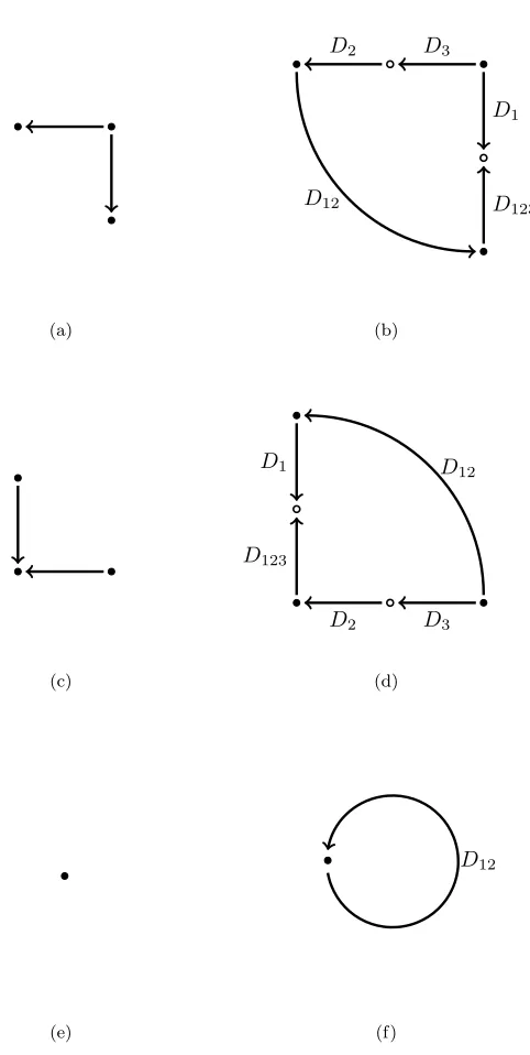
(a)

D2 D3

D1

D123 D12

(b)

(c)

D3 D2

D1

D123

D12

(d)

(e)

D12

(f)

Figure 2.6: CF K∞_{andCF D}\_{for different knots and their framed complements, respectively. (To}

be precise,CF K∞_{(K) is the above diagram tensored withF[U, U}−1_{].) Top,Kis the right-handed}

trefoil, and the framing on the complement is 2τ(K) = 2. Middle, K is the left-handed trefoil,

and the framing on the complement is 2τ(K) =−2. Bottom,Kis the unknot, and the framing is

Chapter 3

Definition and properties of

ε

(

K

)

We will begin by defining the invariantε(K), in terms ofτ(K) and the invariantν(K), defined by

Ozsv´ath and Szab´o in [16, Definition 9.1]. Let (As, ∂s) and (A′s, ∂s′) be the following sub-quotient

complexes ofCF K∞_(K):

As=C{max(i, j−s) = 0}

A′s=C{min(i, j−s) = 0},

with induced differentials ∂s and ∂s′, respectively. We consider both As and A′s as complexes

over F_{. Notice that if {xi} is a basis for CF K}−_{(K), then {U}ni_x

i} is a basis for As, where

ni = max(0, A(xi)−s). Similarly,{Umixi} will be a basis forA′s, wheremi= min(0, A(xi)−s).

We have a mapvs:As→CFd(S3) defined as the following composition:

As→C{i= 0, j≤s} →C{i= 0} ≃CFd(S3)

where the first map is projection and the second is inclusion. Similarly, we have a map vs′ :

d

CF(S3_)→A′

sdefined as the following composition:

d

where the first map is projection and the second is inclusion. These definitions have geometric

significance. Recall from [11, Section 4] that forN ∈N_{sufficiently large,}

As≃CFd(SN3(K),[s])

where SN3(K) denotesN-surgery alongK,|s| ≤N/2, and [s] denotes the Spin c

structures_sthat

extends over the corresponding 2-handle cobordism with the property that

hc1(ss),[Fb]i+N = 2s,

where Fb denotes the capped off Seifert surface in the 4-manifold. The map

vs:CFd(SN3(K),[s])→dCF(S3)

is induced by the cobordism fromS3

N(K) toS3endowed with the Spin

c_{structure above. Similarly,}

A′s≃CFd(S−3N(K),[s]),

and

v′s:CFd(S3)→CFd(S−3N(K),[s])

corresponds to the 2-handle cobordism fromS3 _toS3 −N(K).

Definition 3.1. Defineν(K)by

ν(K) = min{s∈Z_|vs:As→CFd_(S3_{)induces a non-trivial map on homology}.}

Similarly, define ν′_(K)by

ν′(K) = max{s∈Z _|v′

s:CFd(S3)→A′s induces a non-trivial map on homology}.

For ease of notation, we will often writeτforτ(K) when the meaning is clear from context. Recall

from [9, Proposition 3.1] thatν′_{(K) is equal to eitherτ−1 orτ. The idea is that ifs > τ, thenv}′ s

induces the trivial map on homology, because quotienting byC{i= 0, j < s}gives the zero map,

and if s < τ, thenv′

must be supported in the (i, j)-coordinate (0, τ), thusxis not a boundary inA′

s. Thus, we should

focus on the mapv′

τ. In particular,

• ν′_{(K) =τ−1 if and only ifv}′

τ is trivial on homology

• ν′_{(K) =τ if and only ifv}′

τ is non-trivial on homology.

A similar argument shows thatν(K) is equal to eitherτ(K) or τ(K) + 1; in particular,

• ν(K) =τ if and only ifvτ is non-trivial on homology

• ν(K) =τ+ 1 if and only ifvτ is trivial on homology.

We now proceed to show that vτ and v′τ cannot both be trivial on homology. Roughly, the idea

is that v′τ is trivial on homology when the class [x] generating HFd(S3) ∼= H∗(C{i = 0}) is in

the image of the horizontal differential. Thus, [x] must also be in the kernel of the horizontal

differential, implying thatvτ is non-trivial. Similarly,vτ is trivial on homology when [x] is not in

the kernel of the horizontal differential, hence [x] is not in the image of the horizontal differential,

implying that v′

τ is non-trivial.

The following lemma, and its proof, make this precise:

Lemma 3.2. If ν′_{(K) =τ(K)−1, thenν(K) =τ(K), and there exists a horizontally simplified} basis {xi} forCF K−(K)such that, after possible reordering, there is a pair of basis elements,x1

andx2, with the property that:

1. x2 is the distinguished element of some vertically simplified basis.

2. ∂horz_x 1=x2.

Similarly, if ν(K) =τ(K) + 1, then ν′_{(K) =τ(K), and there exists a horizontally simplified basis}

{xi} for CF K−(K) such that, after possible reordering, there is a pair of basis elements,x1 and

x2, with the property that:

2. ∂horz_x 1=x2.

Proof. Let xV be the distinguished element of a vertically simplified basis, and let ∂horzs be the

differential onC{j=s} ≃Chorz_.

Sinceν′_{(K) =τ−1, for any elementxthat generatesH∗(C{i= 0}), we have that [x] = 0∈}

H∗(A′

τ). Thus, there existsx′ ∈A′τ such that∂τ′x′ =xV. Moreover, we may choosex′ to be the

element of minimali-filtration such that∂τ′x′=xV; this will be convenient to us later. (Note that

the complex A′sinherits a naturali-filtration as a subquotient complex ofCF K∞.)

We can write x′ _{as the sum of chains x}

i=0 and xi>0, where xi=0 ∈ C{i = 0, j > τ} and

xi>0∈C{i >0, j=τ}. Furthermore,xi=0 can be taken to be a sum of vertically simplified basis

elements that are not in the kernel of the vertical differential. Hence,

• xV +∂vertxi=0 generatesH∗(C{i= 0})

• ∂′

sxi>0=xV +∂vertxi=0.

We notice that [∂horz

τ xi>0] is non-zero in both H∗(Aτ) and H∗(C{i = 0}). Therefore, ν(K) =

τ(K).

We now need to find an appropriate horizontally simplified basis. ReplacexV with∂τhorzxi>0.

This is a filtered change of basis and this new basis element is still the distinguished element of a

vertically simplified basis, since elements in ∂horz

τ xi>0+xV either havei-coordinate<0, or have

i-coordinate equal to zero and are in the image of∂vert_.

Now apply the algorithm in Lemma 2.8, splitting off the arrow of length, say n, from xi>0

to the newxV first when simplifying Bn. This will yield a horizontally simplified basis with the

desired property.

The proof in the case thatν(K) =τ(K) + 1 follows similarly.

When bothvτ andv′τ are non-trivial on homology, the class [x] generatingHFd(S3), which we

identify with H∗(C{i = 0}), is in the kernel of the horizontal differential but not in the image.

Lemma 3.3. Ifν(K) =ν′_{(K), then there exists a vertically simplified basis{x}

i} for CF K−(K) such that the distinguished element,x0, is also the distinguished element of a horizontally simplified

basis for CF K−_(K).

Proof. Note that ν(K) = ν′(K) implies that both are equal to τ(K). Let {xi} be a vertically

simplified basis{xi} forCF K−(K) with distinguished elementx0. We have the following series

of implications:

1. ν(K) =τ(K) implies there exists a chain xH ∈Aτ such thatvτ∗([xH]) = [x0].

2. Hence, [xH]6= 0∈H∗(Aτ), and so∂τxH = 0.

3. ∂horz

τ xH = 0 as well, since∂τhorzxH =∂τxH/C{i= 0, j < τ}.

Notice that sincevτ∗([xH]) = [x0], it follows thatxH must be equal tox0plus possibly some basis

elements in the image of∂vert _{and some elements inC{i <0, j=τ}. Hence, we may replace our}

distinguished vertical elementx0 withxH.

WithxH is as above,ν′(K) =τ(K) implies thatvτ′∗([xH])6= 0∈H∗(A′τ). Thus,xH ∈/Im∂τ′.

Since xH ∈/ Im ∂τ′, xH is not homologous in C{j = τ} ≃ Chorz to anything of strictly lower

filtration level. Moreover,xH∈/Im∂τhorz. Therefore, there exists a horizontally simplified basis for

CF K−_{(K) with distinguished elementx}

H, which is also the distinguished element of a vertically

simplified basis.

We see that there are three different possibilities for the values of the pair (ν(K), ν′(K)):

(τ(K), τ(K)−1), (τ(K), τ(K)) or (τ(K) + 1, τ(K)). This motivates the following definition:

Definition 3.4. Defineε(K)to be

ε(K) := 2τ(K)−ν(K)−ν′(K).

Remark 3.5. By various symmetry properties of CF K∞_{(K) (see [11, Section 3.5]), we may}

equivalently define ε(K) as

ε(K) = τ(K)−ν(K)− τ(K)−ν(K),

where Kdenotes the mirror ofK.

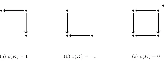
(a)ε(K) = 1 (b)ε(K) =−_{1 (c)}ε(K) = 0

Figure 3.1: CF K∞_{(K), for different knots K. Above left, K is the right-handed trefoil, which}

hasε(K) = 1, and the unique generator with no incoming or outgoing vertical arrows lies at the

head of a horizontal arrow. Center, K is the left-handed trefoil, which hasε(K) = −1, and the

unique generator with no incoming or outgoing vertical arrows lies at the tail of a horizontal arrow.

Right,Kis the figure 8 knot, which hasε(K) = 0, and the unique generator with no incoming or

outgoing vertical arrows also has no incoming or outgoing horizontal arrows.

See Figure 3.1 for examples of knotsK with different values ofε(K). Recall that a knotKis

called homologically thin if HF K\(K) is supported on a single diagonal in the plane whose axes

correspond to Alexander and Maslov gradings of the groups.

Proposition 3.6. The following are properties of ε(K):

1. If K is smoothly slice, thenε(K) = 0.

2. If ε(K) = 0, thenτ(K) = 0.

4. If|τ(K)|=g(K), then ε(K) = sgnτ(K).

5. IfK is homologically thin, thenε(K) = sgnτ(K).

6. (a) Ifε(K) =ε(K′_{), thenε(K#K}′_{) =ε(K) =ε(K}′_).

(b) Ifε(K) = 0, thenε(K#K′) =ε(K′).

Proof of (1). IfK is slice, then the surgery correction terms defined in [8] vanish (i.e, agree with

those of the unknot), and the maps

d

HF(SN3(K),[0])→HFd(S3) and HFd(S3)→HFd(S−3N(K),[0])

are non-trivial. Indeed, the surgery corrections terms can be defined in terms of the maps

HF+(S3)→HF+(S₋3N(K),[s])

and we have the commutative diagram

d

HF(S3₎ vs′

−−−−→ HFd(S3

−N(K),[s]) ι

 

y ι−N,s

  y

HF+(S3₎ u′s

−−−−→ HF+(S3

−N(K),[s]).

Let N ≫ 0. If the surgery corrections terms vanish and s = 0, then u′

s is an injection and so

the composition ι◦u′

s is non-trivial. By commutativity of the diagram, it follows that vs′ must

be non-trivial. A similar diagram in the case of large positive surgery shows that vs must be

non-trivial as well. Thus,ν(K) andν′_{(K) both equalτ(K) = 0, and soε(K) = 0.}

Proof of (2). Ifε(K) = 0, then by Lemma 3.3, there exists an elementx0that is the distinguished

element of both a vertically and horizontally simplified basis. If A(x0) is the Alexander grading

ofx0viewed inCvert≃CF K\(K), then−A(x0) is the Alexander grading ofx0 viewed inChorz≃

\

CF K(K). This implies thatτ(K) =−τ(K), henceτ(K) = 0.

Proof of (3). The symmetry properties of CF K∞_{(K) imply that τ(K) = −τ(K) and ν(K) =}

Proof of (4). Without loss of generality, we can consider the case τ(K)>0. By the adjunction

inequality for knot Floer homology [11, Theorem 5.1],

H∗(C{i <0, j=g(K)}) = 0.

Hence by considering the short exact sequence

0→C{i <0, j=g(K)} →Ag(K)→C{i= 0, j≤g(K)} →0

and the fact that the inclusionC{i= 0, j≤g(K)}֒→C{i= 0}is a quasi-isomorphism (again, by

the adjunction inequality), we see that the mapvg(K):Ag(K)→C{i= 0}induces an isomorphism

on homology. Thusν(K) =τ(K), soε(K) is equal to 0 or 1. Sinceτ(K)>0, it follows thatε(K)

is not equal to zero, and hence is equal to 1.

Proof of (5). In [18, Lemma 5], Petkova constructs model complexes forCF K−_{(K) of}

homologi-cally thin knots, from which the values ofτ(K) andε(K) follow readily.

Proof of (6). Recall from [11, Theorem 7.1] thatCF K−(K#K′)≃CF K−(K)⊗_F[U]CF K−(K′).

We first consider the case whereε(K) =ε(K′) = 1. Then by Lemma 3.2, there exists a horizontally

simplified basis{xi}forCF K−(K) such that

1. x2 is the distinguished element of a vertically simplified basis

2. ∂horz_x

1=Umx2,

and similarly, a horizontally simplified basis{yi}forCF K−(K′) withy2the distinguished element

of a vertically simplified basis, and∂horz_y

1=Uny2. Note thatA(x2) =τ(K) andA(y2) =τ(K′).

ThenA(x2⊗y2) =τ(K) +τ(K′) =τ(K#K′), and [x2⊗y2]6= 0∈H∗(Cvert(K#K′)). Recall the

map

v′s:Cvert→A′s,

and notice that [x2⊗y2] = 0∈H∗(A′τ(K#K′₎(K#K′)) since∂_τ′_(K#K′₎(U−

m_x

1⊗y2) =x2⊗y2.

Henceν′_(K#K′_{) =τ(K#K}′_{)−1, implying thatε(K#K}′_{) = 1. The case whereε(K) =ε(K}′_{) =}

Finally, if ε(K) = 0, then by Lemma 3.3, there exists a basis{xi} for CF K−(K) such that

the elementx0is the distinguished element of both a horizontally simplified basis and a vertically

simplified basis. Then to determine ν(K#K′_{) and ν}′_(K#K′_{), it is sufficient to consider just}

Chapter 4

Computation of

τ

for

(

p, pn

+ 1)

-cables

We will first consider (p, pn+ 1)-cables, whose Heegaard diagrams are easier to work with, and

prove the following version of Theorem 1:

Theorem 4.1. τ(Kp,pn+1) behaves in one of three ways. Ifε(K) = 1, then

τ(Kp,pn+1) =pτ(K) +

pn(p−1)

2 .

If ε(K) =−1, then

τ(Kp,pn+1) =pτ(K) +

pn(p−1)

2 +p−1.

Finally, if ε(K) = 0, then

τ(Kp,pn+1) =       

pn(p−1)

2 +p−1 ifn <0

pn(p−1)

2 ifn≥0.

The proof will proceed as follows. We will determine that only a certain small piece of the TypeD

bordered invariant associated to the framed knot complement is necessary to determine a suitable