University of Pennsylvania
ScholarlyCommons
Publicly Accessible Penn Dissertations
Spring 5-16-2011
Holistic Shape-Based Object Recognition Using
Bottom-Up Image Structures
Praveen Srinivasan
University of Pennsylvania, [email protected]
Follow this and additional works at:http://repository.upenn.edu/edissertations Part of theArtificial Intelligence and Robotics Commons
This paper is posted at ScholarlyCommons.http://repository.upenn.edu/edissertations/307 For more information, please [email protected].
Recommended Citation
Srinivasan, Praveen, "Holistic Shape-Based Object Recognition Using Bottom-Up Image Structures" (2011).Publicly Accessible Penn
Dissertations. 307.
Holistic Shape-Based Object Recognition Using Bottom-Up Image
Structures
Abstract
Object recognition performance that rivals human ability is one of the primary goals of computer vision research. While recognition may take many forms, key tasks include detection, estimating object pose, and segmenting the object from the background. This thesis explores the use of holistic shape matching for recognition using bottom-up image structures such as image segments and contours for all of these tasks. Holistic shape matching utilizes global information about object shape for matching, rather than local image features which often contain too little information to match reliably to the object model.
By examining different tasks related to object recognition, we demonstrate the value of holistic shape matching in a broad range of problems, including perceptual grouping, human pose estimation, and object recognition.
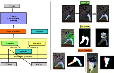
First, we introduce a method for perceptual grouping of contours in an image into larger groups that uses holistic shape matching to estimate the motion of image contours to a second, related image and group them according to similarties in motion. Holistic shape matching provides scoring for different motion hypotheses, and the final grouping is achieved using a min-cut graph cut to infer the cluster assignment for each contour. Secondly, we describe a method for human pose estimation using image segments that incrementally merges segments into hypotheses for increasingly larger regions of the human body. These hypotheses are verified by matching against a set of shape exemplars using a shape matching method that is articulation-invariant and incorporates holistic shape information.
Lastly, we present a two-step method for automatically learning an object detector for an object category from positive and negative images annotated with bounding boxes. In the first step, the object shape is learned from bottom-up image contours extracted in the positive images by searching for ``lucky'' contours that can explain large portions of the shape of positive examples. Given the learned shape, the second step trains a
discriminative
object detector that matches the shape against contours, emphasizing shape features that provide good detection performance. We compare against baselines and previous work that does not use holistic evaluation of shape features to demonstrate its value.
Degree Type
Dissertation
Degree Name
Doctor of Philosophy (PhD)
Graduate Group
First Advisor
Jianbo Shi
Keywords
object recognition, image segmentation, shape, machine learning, computer vision
Subject Categories
HOLISTIC SHAPE-BASED OBJECT RECOGNITION
USING BOTTOM-UP IMAGE STRUCTURES
Praveen Srinivasan
A DISSERTATION
in
Computer and Information Science
Presented to the Faculties of the University of Pennsylvania
in
Partial Fulfillment of the Requirements for the
Degree of Doctor of Philosophy
2011
Supervisor of Dissertation
Jianbo Shi Associate Professor
Computer and Information Science
Graduate Group Chairperson
Jianbo Shi Associate Professor
Computer and Information Science
Dissertation Committee
Kostas Daniilidis Professor of Computer and Information Science
Camillo J. Taylor Associate Professor of Computer and Information Science
Pedro Felzenszwalb Associate Professor of Computer Science, Univ. of Chicago
HOLISTIC SHAPE-BASED OBJECT RECOGNITION
USING BOTTOM-UP IMAGE STRUCTURES
COPYRIGHT
2011
Acknowledgements
No thesis is ever completed in isolation. While many people have played an important
role in my thesis, there are some who deserve special recognition. My parents,
Sampurna and Cidambi Srinivasan, without whose care I never would have come
this far, deserve first billing. From the time I took my first step to receiving my
first diploma, they have been there for me, unwavering in their love and support.
My sister Priyanka, Aunt Uma, Uncle Jayaraman, and my cousins Arun and Vivek
round out my family supporters.
Of course, without a good advisor research can be aimless and mediocre. Thus I
also thank deeply Jianbo Shi, my advisor. His blunt feedback, good and bad, has
critically shaped both my work and my work ethic, pushing me to never settle for
easy answers, to never blindly trod the well-worn path. Also worth mentioning
are Ramesh Gupta and Drago Anguelov, who provided me with some of my first
experiences in academic research.
An ideal academic environment is one with free exchange of ideas, criticisms and
encouragement. Only with a diverse and committed set of fellow students can such an
ideal be fulfilled. My colleagues Timothee Cour, Qihui Zhu, Weiyu Zhang, Katerina
Fragkiadaki, Roy Anati, Gang Song, Ben Sapp, Alex Toshev, Elena Bernardis, Sandy
Patterson, Abhinav Gupta, Yang Wu, Liming Wang, and Spring Berman to name
just a few, have all contributed. Late night discussions, last-minute deadline pushes
and helpful favors from them have also made my life much easier. Qihui deserves
and extraction of image contours, and Weiyu has been a tireless worker in pushing
the efforts in this thesis still further.
My committee members, Kostas Daniilidis, Ben Taskar, C.J. Taylor and Pedro
Felzenszwalb were very helpful in shaping my thesis work and therefore I am
ABSTRACT
HOLISTIC SHAPE-BASED OBJECT RECOGNITION USING BOTTOM-UP
IMAGE STRUCTURES
Praveen Srinivasan
Jianbo Shi, Associate Professor of Computer and Information Science
Object recognition performance that rivals human ability is one of the primary goals
of computer vision research. While recognition may take many forms, key tasks
include detection, estimating object pose, and segmenting the object from the
back-ground. This thesis explores the use of holistic shape matching for recognition using
bottom-up image structures such as image segments and contours for all of these
tasks. Holistic shape matching utilizes global information about object shape for
matching, rather than local image features which often contain too little information
to match reliably to the object model. By examining different tasks related to object
recognition, we demonstrate the value of holistic shape matching in a broad range of
problems, including perceptual grouping, human pose estimation, and object
recog-nition.
First, we introduce a method for perceptual grouping of contours in an image into
larger groups that uses holistic shape matching to estimate the motion of image
contours to a second, related image and group them according to similarties in
motion. Holistic shape matching provides scoring for different motion hypotheses,
and the final grouping is achieved using a min-cut graph cut to infer the cluster
assignment for each contour.
Secondly, we describe a method for human pose estimation using image segments
that incrementally merges segments into hypotheses for increasingly larger regions
of the human body. These hypotheses are verified by matching against a set of
shape exemplars using a shape matching method that is articulation-invariant and
incorporates holistic shape information.
for an object category from positive and negative images annotated with bounding
boxes. In the first step, the object shape is learned from bottom-up image contours
extracted in the positive images by searching for “lucky” contours that can explain
large portions of the shape of positive examples. Given the learned shape, the second
step trains a discriminative object detector that matches the shape against contours,
emphasizing shape features that provide good detection performance. We compare
against baselines and previous work that do not use holistic evaluation of shape
Contents
Acknowledgements iii
1 Introduction 1
1.1 Object Recognition . . . 1
1.2 Shape for recognition . . . 3
1.2.1 Model Representation . . . 4
1.2.2 Features . . . 6
1.2.3 Matching . . . 7
1.3 Layout and Contributions . . . 10
2 Background 13 2.1 Bottom-up Image Structures . . . 13
2.2 Matching Image Structures . . . 14
2.2.1 One-to-one Matching . . . 15
2.2.2 Many-to-Many Matching . . . 15
2.2.3 Many-to-Many Matching Formulation . . . 17
2.2.4 Articulation-Invariant Matching . . . 22
3 Grouping with a Related Image 25 3.1 Related Work . . . 26
3.2 Grouping Criteria . . . 27
3.3.1 Inferring Transformations . . . 30
3.3.2 Many-to-Many Matching for Determining Contextual Shape Information . . . 30
3.3.3 Correspondences using Contextual Shape . . . 31
3.3.4 Baseline Comparison . . . 34
3.4 Experiments . . . 34
3.5 Observations . . . 36
4 Holisitic Human Pose Estimation 38 4.1 Overview of Our Parsing Method . . . 40
4.1.1 Multiple Segmentations . . . 45
4.1.2 Shape Comparison . . . 45
4.1.3 Parse Rule Application Procedure . . . 45
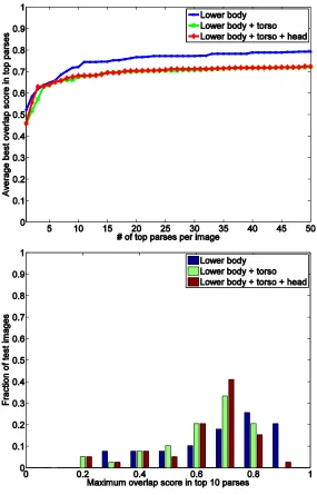
4.2 Results . . . 50
4.2.1 Segmentation Scoring . . . 51
4.2.2 Joint Position Scoring . . . 53
4.3 Observations . . . 55
5 Many-to-one Matching For Describing and Discriminating Object Shape 63 5.1 Overview . . . 64
5.2 Learning a Descriptive Shape Model . . . 67
5.3 Discriminative Detector Learning . . . 72
5.3.1 Object Detection as Many-to-one Matching . . . 72
5.3.2 Latent SVM For Discriminative Detector Learning . . . 75
5.3.3 Placement Refinement and Joint Matching . . . 76
5.4 Experiments . . . 80
6 Conclusion 93
6.1 Summary . . . 93
List of Tables
5.1 Detection rates on ETHZ Shape Classes dataset. . . 85
5.2 Average precision on ETHZ Shape Classes dataset. . . 86
5.3 Ablative analysis of different method components. . . 86
List of Figures
1.1 Three goals of recognition: detection, alignment and segmenting
ob-ject boundaries. . . 2
2.1 Shape recognition requires matching of image contours. . . 14
2.2 Overview of the many-to-many matching process. . . 16
2.3 Encoding of contours for many-to-one matching. . . 19
2.4 Matching score of many-to-one matching. . . 20
2.5 Examples of many-to-one matching. . . 21
2.6 Inner-distance shape context computation. . . 24
3.1 Grouping with a related image. . . 26
3.2 Proposing transformations via SIFT feature matches. . . 31
3.3 Overview of correspondence process. . . 33
3.4 Baseline comparison and additional results. . . 35
4.1 Goals of human pose estimation. . . 39
4.2 Body parse tree. . . 43
4.3 Parse rules. . . 44
4.4 Need for holistic evaluation of object shape. . . 44
4.5 Multiple segmentations. . . 46
4.6 Body parsing procedure. . . 47
4.7 Quantitative segmentation results. . . 52
4.9 Additional pose estimation results. . . 57
4.10 Top 5 parse results for each test image. . . 58
4.10 Top 5 parse results, continued. . . 59
4.10 Top 5 parse results, continued. . . 60
4.10 Top 5 parse results, continued. . . 61
4.10 Top 5 parse results, continued. . . 62
5.1 Overview of our proposed method for learning an object detector. . . 65
5.2 Model shape learning process. . . 66
5.3 Shape models learned from ETHZ Shape Classes dataset. . . 70
5.4 Overview of discriminative tuning of many-to-one matching score func-tion. . . 71
5.5 Affine transformation of image to model improves alignment. . . 78
5.6 Precision-recall and FPPI-detection rate curves for our method. . . . 83
5.7 Examples of detection results on ETHZ Shape Classes dataset. . . 84
5.8 Listing of detection results for each class. . . 88
5.8 Listing of detection results for each class. . . 89
5.8 Listing of detection results for each class. . . 90
5.8 Listing of detection results for each class. . . 91
Chapter 1
Introduction
1.1
Object Recognition
A long-held goal of computer vision has been recognition of a wide variety of objects
in complex, cluttered images, an everyday task humans perform with ease. Although
there are many different tasks that comprise the recognition problem, three
impor-tant tasks (Figure 1.1) include detection, alignment and segmentation:
• Detection: indicating the presence or absence of an object at a particular
location in the image.
• Alignment: determining the pose of an object by corresponding it to a shape
model.
• Segmentation: in order to understand how to manipulate or interact with an
object, we must be able to determine the boundaries of the object.
There are many different applications that can benefit from accurate object
recog-nition, including robot navigation, web image search, video analysis and medical
image understanding. However, despite substantial progress, the problem remains
unsolved. One promising area of focus concerns the use of object shape to
Detect
Align
Segment
Test image
Figure 1.1: Three goals of recognition: detection, alignment and segmenting object boundaries.
represent commonalities of different instances of a particular object category, while
preserving enough detail about objects in order to differentiate them from each other
or the background. It also varies systematically with 3D viewpoint, enabling
esti-mation of the object pose from shape, and segmentation is exactly determining the
object shape boundary. While there are many different approaches to using object
shape for recognition, there are two difficulties faced by nearly all approaches: object
pose variation and the presence of background clutter.
• Background clutter: nearby regions or edges in the image may belong to objects
in the background. Shape feature descriptors computed on the boundary of
the object can therefore be corrupted by these background objects.
• Object pose variation: many objects, such as articulated objects (e.g. humans),
or deformable objects vary in appearance according to pose. As a result, the
relative positions of important shape features may vary substantially.
Given these challenges, we can characterize the recognition problem into four
No pose variation, no background clutter: Object shape features appear clearly
in this scenario, and discriminatively trained object detectors can identify clear
fore-ground shape features to detect objects.
Pose variation, no background clutter: When only pose variation is present,
bottom-up image segmentation can yield clear foreground segments with large
por-tions of the object boundary shape. These segments can be used to infer the
artic-ulated pose of the object and achieve articulation invariant recognition.
No pose variation, background clutter: If background clutter is present
with-out pose variation, relative spatial relationships between foreground shape features
and background clutter areas remain consistent. Therefore, discriminatively trained
detectors can emphasize areas that consistently contain foreground object shape
features while simultaneously ignoring areas that consistently contain background
clutter.
Pose variation, background clutter: This case is in a separate category from
the rest, as the spatial relationships of shape features and clutter vary along with
the object pose. Therefore, bottom-up image segmentation fragments unpredictably,
while the relative positions of shape features and background clutter vary with object
pose. As a result, none of the previous assumptions necessary for applying the
aforementioned strategies are satisfied.
In complex, real-world images, the last case is the norm and not the exception.
Focusing on this setting of recognition, we can analyze different approaches to
shape-based object recognition in terms of how they address these two problems.
1.2
Shape for recognition
There are three important areas that must be addressed in using shape for object
recognition: representation of the shape model, shape features used for matching,
come with different trade-offs among computational efficiency, tractability of good
approximate or exact inference, and learnability of good cost functions for
recogni-tion, as well as addressing the recognition challenges outlined above.
1.2.1
Model Representation
On the model side, there are many different methods for representing object shape.
Broadly speaking, representations in the early history of computer vision research
tended towards greater abstraction, representing objects in terms of high-level
con-cepts such as geometric shapes (2-D primitives such as lines and curves, and 3-D
primitives such as rectangular prisms and conic sections) or other semantic categories
(e.g., an airport is composed of a runway and a terminal building). Unfortunately,
the semantic gap between these abstract representations and the image pixels has
proven to be difficult to bridge directly. As a result, vision research in recent years
has focused on much simpler template representations of objects. Templates do not
capture the same general properties of object shape, but are much easier to compare
against image features than abstract representations. However, because they are not
as general template models are not as compact as abstract representations (e.g., for
viewpoint invariant recognition, Basri et al. [4] used multiple 2-D templates). We
discuss examples of the two types of model representations:
Abstract Representations
Generalized cylinders: Consisting of a set of cross-sectional shapes and a path
that joins their centers of gravity, the generalized cylinder is the shape formed by
resulting volume formed from the cross-sectional shapes. Proposed by Binford ([9]),
generalized cylinders can represent a wide variety of different object shapes.
Geons: Biederman ([8]) proposed geons, a set of simple 3-D geometric shapes that
can be combined together to form a wide variety of 3-D object shapes, similar to the
all geons possess - view-invariance: each geon can be identified when seen from any
viewpoint; stability: under occlusion or deformation, geons are still recognizable; and
discriminability: two different geons can be visually distinguished from one another,
regardless of viewpoint or occlusion.
AND-OR Graphs: To address some of the issues of previous abstract models,
AND-OR graphs [13] were proposed as an object model that contains multiple levels
of abstraction, from the image pixels all the way up to abstract parts of objects.
Specifically, AND-OR graphs are a type of graph with two types of nodes: AND
nodes and OR nodes. AND nodes represent inclusion of all children nodes as part of
the object, while at each OR node, one child is selected to be part of the object. As
a result, AND-OR graphs can compactly represent substantial object variation in a
single model. For example, a chair may be composed of a back, base and bottom;
each of these can have multiple different appearances depending on the specific type
of chair, and each may decompose further into object subparts.
Template Representations
Deformable 2D templates: A simple form of object representation, the 2D
tem-plate may consist of a set of contours or weights on histogram bins (a histogram
computed on either the outline of the shape or gradients of image examples of the
object) to represent the shape of an object from a single view, in a single pose. By
combining a collection of 2D templates of an object imaged from different viewpoints,
3D object recognition can be achieved as demonstrated by Basri [4].
Articulated templates: For articulated objects, a simple deformable template
is insufficient to capture all of the possible deformations of the object. Instead, a
model that explicitly takes into account the articulated nature of the object can help.
The most popular example is the pictorial structures model of Fischler & Elschlager
[27], popularized by Felzenszwalb and Huttenlocher [24], which consists of a set of
non-articulated deformations. An efficient inference method for pictorial structures
models was proposed in [24] and was used to estimate the pose of the human body
(locating the limbs) and faces (locating the eyes, nose mouth).
In this thesis, we focus on template representations of objects, using bottom-up image
structures as a mid-level representation between the object model and the image.
Future work would include introducing increasingly abstract model representations
using perceptual structures such as image segments, contours and junctions as a
mid-level representation between the abstract representations and the image.
1.2.2
Features
In order to use object shape for recognition, we require a method for computing
statistics about the shape that can be compared with the image in order to find
shape matches in the image. These image features allow us to compare the template
models of objects against bottom-up image structures. Various shape features have
been proposed to address this problem:
Shape context: Belongie et al. ([5]) introduced the shape context descriptor for
matching of rigid templates in 2-D images. The shape context is a log-polar spatial
histogram over the location of edges in an image. Smaller bins near the center of the
descriptor capture local, precise shape details, while larger bins further away capture
more general statistics about the overall object shape. Multiple shape contexts can
be computed at different locations in the image and model, and then these shape
contexts can be matched by a variety of methods, including the Hungarian method.
However, clutter may corrupt the descriptor in complex scenes, resulting in poor
match scores despite the actual object of interest being present.
Inner-distance shape context: Related to the shape context, the inner-distance
shape context (IDSC) proposed by Ling et al. ([41]) is again a histogram over the
locations of object boundary points, but is computed in a way as to be invariant to
through the interior. The length of this path and the local orientation of the object
shape at each of the boundary points are used to compute an articulation-invariant
descriptor (described in further detail in Chapter 2). The IDSC was used for shape
matching of silhouette images for shape retrieval in [41], and was also used for human
pose estimation in [62].
HOG feature: The Histogram of Oriented Gradients, or HOG feature ([18]), is
a histogram over gradient orientations in a particular region of the image. These
gradients can capture local shape features of an object, for example the shape of a
person’s head, or the appearance of a body limb. Similar to the shape context, the
descriptor can be corrupted by background clutter. For this reason, the descriptor
support is typically very small relative to the overall object size, limiting the scale
of shape features that can be represented. The descriptors are often scored using
a set of linear weights learned discriminatively, e.g. from a support vector machine
(SVM), that emphasize the important local features of object shape for good
de-tection performance. The HOG feature was applied to pedestrian dede-tection by [18],
where weights on the individual features were learned via linear SVM from positive
and negative instances of pedestrians in a dataset of outdoor street scenes.
1.2.3
Matching
Given shape features in the image, these features must be matched against the object
shape model in order to achieve recognition. This typically involves at least
align-ment of the model to the image, and may also include segalign-mentation of the object.
Many different methods for shape matching have been developed, implementing a
variety of different cost functions with corresponding trade-offs in computational
Template Matching Using Local Features
Chamfer matching/Distance transform: Given a template representation of
an object consisting of a set of points that represent the object boundary, chamfer
matching using the distance transform can be used to evaluate the matching of
the template at a particular location in the image. A placement (represented by a
translation) of a 2D object template in an image can be scored by computing the
distance of each point in the template to the closest edge in the image, under the
specific placement. These distances can be summed to provide a score for placing an
object at a particular location in the image. The distance transform of [23] can be
used to efficiently compute this score at all possible placements of the template in
the image. While chamfer matching is a very fast method for computing a matching
score at many locations in an image, clutter in the image can cause many false
matches since the more image edges that are present, the more likely a point in the
template will have an image edge nearby. Active shape models ([14]) have a similar
cost function for matching, but allow for deformation of the model shape via a linear
basis for the shape learned from training example shapes.
Local features + pairwise geometric constraints: Another simple method for
shape matching is using local image features, computed by the similarity of a set
of model weights with a set of image features extracted at a particular location in
the image, measured by correlation. For example, the image features might be HOG
features, while the weights may have been learnt through a discriminative procedure,
as in [18]. Multiple object parts can be detected in the image using this method and
their scores can be combined via voting for the object center using the known spatial
relationships of the parts relative to the object center, as in [22]. Arbitrary pair-wise
relationships can also be incorporated, as did Coughlan and Ferreira ([15]), using
Abstract Representation Matching
Interpretation tree: The interpretation tree, introduced by Gatson and
Lozano-Perez in [29], is a formalism for structuring the search space of correspondences
between an image and a set of object models. Each edge in the tree represents
an additional correspondence of image points to the object model, and typically
edges emanating from the ith level of the tree represent possible correspondences of
the ith point to different points on the various object models. A leaf in the tree
represents an interpretation, or assignment of image points to object models. Not
all leaves represent valid interpretations; for example, in rigid object recognition
from range images, there must exist plausible 3-D transformations that can align
the object models with the corresponded image points. The interpretation tree is
very general, and is capable of matching any image against virtually any object
type of object model. Unfortunately the number of possible interpretations is in
general exponential in the number of image points, making interpretation tree search
(exploration of all possible leaves) impractical for complex scenes with many image
points/object models.
Holistic Matching
Many-to-many matching: Bottom-up image segmentation can yield important
image structures that are useful for object recognition. However, these image
struc-tures may fragment in unpredictable ways, resulting in no possible one-to-one
cor-respondence between image structures and object parts. Several researchers have
explored the concept of many-to-many matching as a way of dealing with this
frag-mentation problem. Demirci et al. [19] formulated the many-to-many matching
problem between two graphs by first finding an embedding of nodes of each graph
using a low-distortion graph embedding technique, followed by solving an Earth
Mover’s Distance (EMD; [55]) problem where the flows between nodes were
graphs of silhouette images for shape matching.
Zhu et al. [73] developed an alternative approach for many-to-many matching based
on linear programming. Given two sets of contours, the goal was to find a
sub-set of contours in each that had similar shape. Shape similarity was measured by
comparing shape contexts computed over the selected subsets of contours, and a
computationally efficient approximation to this combinatorial problem was
formu-lated as a linear program. The many-to-many matching was used to detect object
parts in the image, which were then combined via a voting scheme to provide object
detection scores. The approach was evaluated on the ETHZ Shape Classes dataset
from [25], and showed good detection performance.
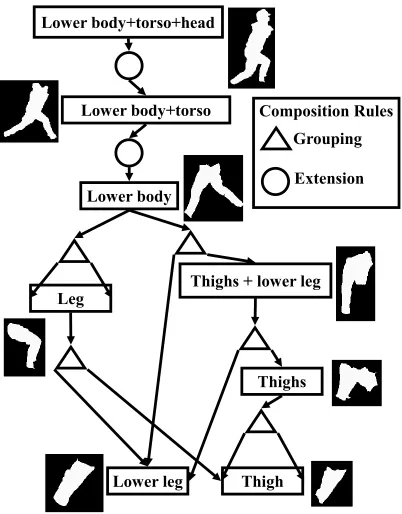
Many-to-one matching: Discussed further in Chapter 4, this thesis introduces a
method for many-to-one matching of image segments to an object model, specifically
for human pose estimation. For the human body, different shape exemplars were
specified for different regions of the body. Because the human body is compositional
in nature, proposals for a particular body region were created by combining proposals
from subregions. For example, to form a proposal for the lower body, a single
segment could be taken, two proposals for legs could be combined, or a proposal for
three-fourths of the lower body and a lower leg (the remaining one-fourth) could be
combined. Because these proposals consist of image segments, a region of the body
could be formed by combining one or more image segments together. Evaluation of
the proposals was achieved by shape matching of these proposals to shape exemplars
via the inner-distance shape context to achieve articulation invariant matching.
1.3
Layout and Contributions
From the above discussion, it is clear there are many different possible approaches
to object recognition, using one or more of the previous ideas. In this thesis, we
matching of bottom-up image structures such as contours and segments to an object
shape model. In particular, holistic evaluation of bottom-up image structures is
well suited to addressing the challenges of pose variation and background clutter.
We demonstrate the application of these ideas to a variety of different problems in
recognition, as well as superior performance due to the use of holistic evaluation of
shape:
• Chapter 2 reviews several different methods for holistic evaluation of object
shape, including the works of Zhu et al. [73], many-to-many matching, and
Ling et al. [41], articulation-invariant shape evaluation.
• Chapter 3 discusses perceptual grouping. We introduce a method for grouping
of image contours into larger clusters using many-to-many matching to
estab-lish accurate correspondences, thereby estimating the motion of contours and
grouping contours with similar motions into the same group. Final group
as-signment is achieved using a min-cut graph cut that derives its unary scores
from the many-to-many matching score of a contour in one image to another
under a specific motion hypothesis.
• Chapter 4 studies human pose estimation. In this chapter a method for
esti-mating human pose using bottom-up parsing of image segments is described.
The overall cost function for evaluating human pose hypotheses is non-additive,
allowing for evaluation of holistic shape properties of groups of image segments
that cannot be observed from the individual segments. Proposals for regions
of the human body are evaluated by matching against shape exemplars using
an articulation-invariant shape matching method; as a result, few exemplars
are needed to be able to match a wide range of articulated human shapes.
• Chapter 5 addresses generic object recognition. For a specific object category,
object shape is automatically learned from the image contours of positive
learned shape model and the contours of positive and negative images. The
re-sult is a fully automatic system for learning an object detector that can detect
a specific object category in a new image using bottom-up image contours. A
key characteristic of both the shape learning as well as the object detection
is the use of many-to-one matching for holistic shape evaluation of detection
hypotheses as well as candidate image contours for constructing the model
shape.
• Chapter 6 concludes with a summary of the work in this thesis as well as a
Chapter 2
Background
2.1
Bottom-up Image Structures
One of the key themes of this thesis is the use of bottom-up image structures for
grouping and recognition. Such structures naturally capture long-range grouping
constraints between pixels or edges that can constrain and improve both tasks. There
are two primary types of structures, image segments and image contours. An image
segment consists of a subset of the pixels in the image, typically contiguous, and
may often correspond to a portion of an object. For extracting segments, we use
the method of Cour et al. ([16]), which uses the normalized cuts algorithm ([57]) to
partition a graph over image pixels into multiple regions. The graph includes both
short-range and long-range connections, where connection weights are determined
using the intervening contour cue (the magnitude of the strongest edge that lies
between two pixels). Multiple image segmentations can be produced by varying
parameters such as the number of segments produced by the segmentation method,
representing different hypotheses for groupings of image pixels.
An image contour is an ordered set of edge pixels in an image. Long contours often
contain important information about the figure-ground boundary of an object or its
?
a)
b)
c)
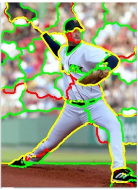
Figure 2.1: Recognizing an object by shape using image contours requires matching a subset of image contours against an object model. From an image (a) bottom-up contours are extracted (b), which then need to be matched against a shape model (c). Most of the image contours do not correspond to the object of interest, and those that do fragment unpredictably.
et al. ([72]). The approach first begins with edge detection in the image, keeping
edges above a low threshold on the edge strength. A directed graph is formed
over these edges, where the graph weights are determined by geometric consistency
of neighboring edges (edges with similar orientations have stronger connections).
Complex eigenvectors are computed from the weighted adjacency matrix for the
graph, and for each of these eigenvectors, cycles are traced in the complex plane to
find individual contours. The resulting contours may overlap, representing different
grouping hypotheses at junctions in the image.
2.2
Matching Image Structures
Given a set of image structures, recognition typically requires matching these
struc-tures against an object model. For example, Figure 2.1 shows an image with
ex-tracted contours that we wish to match against an outline model of the object.
There has been substantial work on this topic, but we focus here on two types of
methods for matching, one-to-one matching and many-to-one matching, that have
2.2.1
One-to-one Matching
One of the most common approaches to matching is one-to-one matching, where each
model structure is matched to at most one image structure. There have been many
approaches ([17, 40, 65, 31, 5]) which minimize similar cost functions that typically
consist of unary terms indicating the direct compatibility of a match, and pairwise
terms indicating the compatibility of pairs of matches. Because of the nature of
these cost functions, only local relationships relating to a small region of the object
or pairs of small regions are captured. Holistic characteristics of the object shape are
not easily captured with one-to-one matching cost functions. Figure 2.1 illustrates
an example of one-to-one matching being insufficient for matching image contours
to an object shape model. Because the contours of different instances of a particular
object category may fragment very differently in the image, there is no one-to-one
correspondence of these contours to the object model, and keeping around all possible
fragmentations of object contours is intractable.
2.2.2
Many-to-Many Matching
Because one-to-one matching is insufficiently flexible to handle the matching of
bottom-up structures that fragment unpredictably, researchers have developed
meth-ods for many-to-many matching. A many-to-many matching maps subsets of a set
Ato subsets of a set B. The advantage of many-to-many matching is that groups of
image structures can be holistically matched to the object model without regard to
their specific fragmentation. The contours corresponding to the outline of the object
in the image could be fragmented arbitrarily, yet many-to-many matching would
be able to match them to the object shape model with the same cost. Demirci et
al. [19] formulated the many-to-many matching problem between two graphs by first
finding an embedding of nodes of each graph using a low-distortion graph embedding
technique, followed by solving an Earth Mover’s Distance (EMD) problem where the
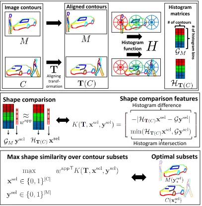
1 2 2 1 1 1 2 2 1 1 2
1, ) || || ||min( , )||
( ost
SelectionC c c SCc SCc L SCc SCc L
2 1 c m c1 1 1 c 2 2 c n c2 1 2 c i j c j i cij{0,1}[0,1] ,
j i ci
j [0,1] ,
s.t. ) c , ost(c SelectionC 1 2 c , c min 2 1 T m c c c c [ 2... 1]
1 1 1 1 T n c c c c [ ... 2]
2 2 1 2 2
≈
# of his
togr
am
bins
# of contours
Image contours Aligning transf-ormation Aligned contours Histogram function
Shape comparison features
Max shape similarity over contour subsets
Optimal subsets
Shape comparison
Histogram matrices
Histogram difference
Histogram intersection
Figure 2.2: Overview of the many-to-many matching process. Top: two sets of
contours M and C are provided as input. An aligning transformation T transforms
contours C such that some object(s) align between the two sets of contours. A
histogram function H operates on the contoursM and transformed contours T(C),
producing a histogram for each contour, which appears as a column of matrices
GM and HT(C). Middle: our goal is to infer indicator vectors xsel,ysel that specify
a specific subset of contours in the two sets such that the two subsets have similar histograms (and hence shape). To compare histograms, we use histogram comparison
featuresK(T,xsel,ysel), a function of the transformationTand the contour subsets.
Bottom: our goal is to maximize the similarity of the two histograms over the choices of subsets of contours to match the contours of the common aligned object (a car
in this instance). The two quantities xsel
∗ and y∗sel together are the optimal solution
their method to match shock graphs of silhouette images for shape matching.
Zhu et al. [73] developed an alternative approach for many-to-many matching based
on linear programming. Given two sets of contours, the goal is to find a subset of
con-tours in each that had similar shape. Shape similarity was measured by comparing
shape contexts computed over the selected subsets of contours, and a
computation-ally efficient approximation to this combinatorial problem was formulated as a linear
program. The many-to-many matching was used to detect object parts in the image,
which were then combined via a voting scheme to provide object detection scores.
The approach was evaluated on the ETHZ Shape Classes dataset from [25], and
showed good detection performance. An advantage of this approach over [19] is that
it does not require explicit specification of a distance between contours in the two
sets, which can be difficult to specify when one contour overlaps only partially with
the other.
2.2.3
Many-to-Many Matching Formulation
Following Zhu et al. [73], we formulate a computational solution to the
many-to-many matching problem for matching object shape. In the contour setting, we are
given a set of model contours M and image contours C, and wish to find a subset
of each such that the overall shapes of the two subsets is similar. To characterize
the shape of the subsets, we can use any spatial histogram, such as one or more
shape contexts [6], or a grid histogram. Figure 2.2 shows an example with several
different shape contexts used together as a single histogram. During matching, we
must find both the subsets of contours in the model and the image as well as an
aligning transformation that aligns the image contours to the object shape model so
that shape similarity can be measured accurately. These quantities can be defined
as:
• T∈ R2: a transformation that describes the alignment of the image contours
• xsel ∈ {0,1}|C|: an indicator vector that defines which image contours are
selected for matching to the model. Contour Ci is selected if and only if
xsel
i == 1.
• ysel ∈ {0,1}|M|: an indicator vector that defines which model contours are
selected for matching to the image. Contour Mi is selected if and only if
ysel
i == 1.
Figure 2.2, top, shows a set of contours in two images as input to the matching;
an aligning transformation T aligns the two sets of contours. We define a spatial
histogram of dimension dm over the edge points of image contours selected by xsel
and transformed by T as: hT(C),xsel. Any type of spatial histogram is allowed,
including grid histograms (as used in [18]) or log-polar radial histograms (as in [6]).
We encapsulate this property via a histogram function H, which maps a point in
R2 to a vector in Rdm, or H : R2 → Rdm. In general, any possible histogram is
permitted as long as it satisfies the following property: given two sets R and S and
the histogram function H, we require: H(R ∪S) + H(R ∩S) == H(R) +H(S).
Specifically in this case, a histogram over the points of several contours is equivalent
to summing the histograms computed for each contour individually, first noted in
[73], and also depicted in Figure 2.3. This means that histogram hT(C),xsel can be
represented as a linear function of xsel as shown in Figure 2.3. We introduce the
per-contour histogram matrix HT(C) (Figures 2.2 and 2.3) and write the histogram
over selected-contours hT(C),xsel as a linear function of xsel:
HT(C) ∈Rdm×|C| hT(C),xsel ⇐⇒ HT(C)xsel (2.1)
The k-th column of HT(C) is a histogram over the points in contour Ck. Similarly,
we can also represent the model contour shape contexts with a matrix GM, where
each column is a shape context for a model contour. To compare the histograms that
1
2
1
Per-contour histogram matrix*
=
0 1*
=
1 1=
1 0*
2
Figure 2.3: Encoding of contours for many-to-one matching. Left, two contours, are shown with associated histograms (any histogram, grid or shape context, is
possible), which are combined to form matrixHT(C)(center). Right, different choices
of selection vectorxsel lead to different histograms;h
T(C),xsel is thus a linear function
of xsel.
types of features: bin-wise difference features −|HT(C)xsel− GMysel|and intersection
features min(HT(C)xsel,GMysel).
K(T,xsel,ysel) =
−|HT(C)xsel− GMysel|
min(HT(C)xsel,GMysel)
(2.2)
Figure 2.2, middle, shows the comparison of the two histograms resulting from
choos-ing a subset of contours in both the model and image, and the features used for
histogram comparison. Given a weighting on these features wapp ≥0, our goal is to
solve the maximization problem:
max
xsel ∈ {0,1}|C|
ysel ∈ {0,1}|M|
wappTK(T,xsel,ysel) (2.3)
An important question is how to perform the above maximization over T,xsel,ysel.
Many
contours?
Similar
shape?
x
x
Different possibilities for , given
Figure 2.4: Matching score of many-to-one matching. For a given model shape
(upper left; Giraffe) and placement T, different selections xsel of image contours
are shown. Indicator xsel encodes which image contours are many-to-one matched.
Matching score prefers selections and placements that select many contours which have similar shape to the model.
can solve (or approximate) this integer linear program, we can directly search over
different possible choices ofT, solving a separate optimization problem for each one.
Instead of trying to solve the integer linear program exactly, we can relax xsel ∈
[0,1]|C|andysel ∈[0,1]|M|, resulting in a linear program that can be solved efficiently
via a linear program solver ([2]), as in Zhu et al. [73]. With the restriction ofwapp ≥
0, this score function is concave and maximization is possible. We can write a linear
program that maximizes a relaxation of our score functionwappTK(T,xsel,ysel) using
proxy variablesm and oto represent the histogram difference −|HT(C)xsel− GMysel|
Figure 2.5: Examples of many-to-one matching. Left: input image; center: two different points on model to be matched in the image; right: different many-to-one matchings of model to image. A single shape context was used as the histogram,
centered at the highlighted points on the model; the transformation T relating the
max
xsel∈[0,1]|C|
,ysel∈[0,1]|M| w
appT
m
o
s.t. m ≤(GMysel− HT(C)xsel),(HT(C)xsel− GMysel)
o ≤ HT(C)xsel,GMysel
(2.4)
Many-to-one Matching: An important special case of the many-to-many
match-ing problem is the many-to-one matchmatch-ing problem. In this settmatch-ing, instead of havmatch-ing
multiple model contours, there is just one, which must always be matched (cannot
be de-selected). The variables for model contour selection ysel can be eliminated,
and the term Gysel can be replaced with a single model histogram h
M.
Figure 2.4 shows examples of different possible selections xsel and how the
many-to-one matching cost function behaves as a result, while Figure 2.5 shows examples of
many-to-one matchings of different points on an object model to an input image.
2.2.4
Articulation-Invariant Matching
The previously described many-to-one matching handles only the case of largely
rigid objects. However, many interesting object categories such as humans are
artic-ulated and therefore we require a different approach to matching bottom-up image
structures to the object model in the case of articulation. The inner-distance shape
context (IDSC) was proposed by Ling et al. ([41]) as a descriptor capable of
ad-dressing this issue. One way to use the IDSC is for matching bottom-up segments
in an image against exemplar shapes of different regions of the body. Because the
IDSC is largely invariant to articulation, image segments can still be matched to the
exemplars even if the pose of the person in the image is different than that of the
exemplars.
The IDSC is an extension of the original shape context proposed in [6]. In the
original shape context formulation, given a contour of n points x1, ..., xn, a shape
#(xj, j 6=i:xj −xi ∈bin(k)) (2.5)
Ordinarily, the inclusion functionxj−xi ∈bin(k) is based on the Euclidean distance
d =k xj −xi k2 and the angle acos((xj −xi)/d). However, these measures are very
sensitive to articulation. The IDSC replaces these with an inner-distance and an
inner-angle.
The inner-distance between xi and xj is the shortest path between the two points
traveling through the interior of the mask. This distance is less sensitive to
articu-lation. The inner-angle between xi and xj is the angle between the contour tangent
at the point xi and tangent at xi of the shortest path leading from xi toxj. Figure
2.6 shows the interior shortest path and contour tangent.
The inner-distances are normalized by the mean inner-distance between all pairs
{(xi, xj)}, i 6= j of points. This makes the IDSC scale invariant, since angles are
also scale-invariant. The inner-angles and normalized log inner-distances are binned
to form a histogram, the IDSC descriptor. For two shapes with points x1, ..., xn
and y1, .., yn, IDCSs are computed at all points on both contours. For every pair of
points xi, yj, a matching score between the two associated IDCSs is found using the
Chi-Square score ([6]). This forms an n-by-n cost matrix, which is used as input
to a standard dynamic programming algorithm for string matching, allowing us to
establish correspondence between the points on the two contours. The algorithm also
permits occlusion of matches with a user-specified penalty. We try the alignment at
several different, equally spaced starting points on the exemplar mask to handle the
cyclic nature of the closed contours, and keep the best scoring alignment (and the
score). The complexity of the IDSC computation and matching is dominated by the
matching; with n contour points and s different starting points, the complexity is
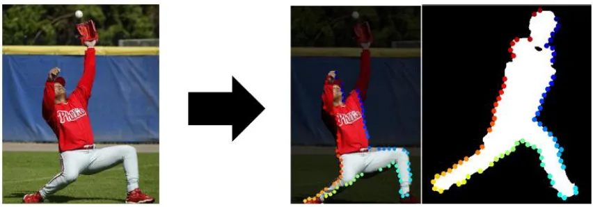
Figure 2.6: Inner-distance shape context computation. Left: We show: shortest interior path (green) from start (blue dot) to end (blue cross); boundary contour points (red); contour tangent at start (magenta). The length of interior path is the inner-distance; the angle between contour tangent and the start of the interior
path is the inner-angle. Center: Lower body mask parse; colored points indicate
Chapter 3
Grouping with a Related Image
As mentioned in Chapter 1, bottom-up image structures are useful for addressing the
pose variation and clutter challenges of object recognition. However, the process of
bottom-up grouping is itself susceptible to corruption by these issues. For example, in
segmentation by motion or stereo, correspondences between pairs of images must be
established in order to estimate the motion of different parts of the image. Typically
this is achieved using matching of local image patch features ([58, 67, 69]). As
discussed previously, local features can be corrupted by background objects and
object deformation and therefore be poorly matched between pairs of images. In
this chapter, we introduce a method for perceptual grouping based on a pair of
related images that addresses the issues of background clutter and object deformation
using holistic evaluation via many-to-many matching of image contours between the
images.
The pair of images may be a stereo pair, frames from a video, or two similar images
(images containing similar objects). Relative motion of contours in one image to
their matching contours in the other provides a cue for grouping - contours that
undergo similar motion should be grouped together. The contours themselves are
detected bottom-up without a model, and are provided as input to our method.
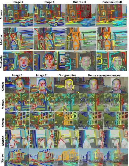
Stereo Motion Similarity
Grouping in image 1 using related images
Imag
e 1
Imag
e 2
Figure 3.1: Contours (white) in the image on the left can be further grouped using the contours of a second, related image (top row). The bottom row shows idealized groupings in the original image according to the inter-image relationship.
large spatial support. Region segments, on the other hand, have large spatial
sup-port, but lack the structure that contours provide. Therefore, additional grouping
of contours can give us both qualities. This has important applications for object
recognition and scene understanding, since groups of contours are often large pieces
of objects.
Figure 3.1 shows a single image in the 1st column, with contours; in the other
columns, top row, are different images related by stereo, motion and similarity to the
first, shown with their contours. Below each of these images are idealized groupings
of contours in the original image. Note that internal contours on cars and buildings
are grouped, providing rich, structured shape information over a larger image region.
3.1
Related Work
Stereo, motion, and similar image matching have been studied largely in isolation,
and often with different purposes in mind than perceptual grouping. Much of the
can be used for perceptual grouping, with the advantage that precise depth
estima-tion is not required to infer a good grouping. Moestima-tion is often used for estimating
optical flow or dense segmentation of images into groups of pixels undergoing similar
motion [68]. These approaches to motion and stereo are largely region-based, and
therefore do not provide the same internal structure that groups of contours provide.
Similar image matching has been used for object recognition [7], but is rarely applied
to image segmentation.
In work on contours, Sherman and Peleg ([56]) matched contour points in the
con-text of aerial imagery, but use constraints such as ordering of matches along scanlines
and disparity gradient that are not appropriate for motion or similar images, and
do not provide grouping information. Liu et al. [42] grouped image pixels into
con-tours according to similar motion using optical flow as a local cue. While the result
addresses the long-standing aperture problem in motion estimation, the framework
does not extend to large inter-image deformations or matching across similar images.
Hedau et al. [34] grouped and matched image regions across different images and
unstable segmentations (as we do with contours), but the regions lack internal
struc-ture. Others ([10, 30]) used stereo pairs of images to detect depth discontinuities
as potential object boundaries. However, these methods will not detect and group
group contour points in the interior of fronto-parallel surfaces.
3.2
Grouping Criteria
We first present some definitions and our basic criteria for grouping contours. The
inputs to our method are:
1. Images: I1,I2; for each image Ii we also have:
2. A set of points (typically image edges) Pi ⊂R2. We restrict the set of points
3. A set of contours Ci, where Cij ∈ Ci is an ordered subset of points in Pi:
Cij = [Pk1 i , P
k2 i , ..., P
kn
i ]⊆Ci.
Our goal is to assign each contour in the first image I1 to a group 1, ..., n. For each
contour C1j, we create a label variable lj ∈ {0,1, ..., n}, where lj == 0 means the
contour is ungrouped, and value k ∈ {1, .., n} means the contour belongs to group
k. The collective set of all label variables is denoted as L.
We would like the groups to possess the following criteria:
1. Good continuation - for contours that overlap significantly, we prefer that they
are present in the same group, if they are grouped at all. For overlapping
contours Ci
1, C j
1, we prefer that li ==lj.
2. Common fate by shape: each contour point in a grouped contour should be
matchable to a point in the second image where the local shape of the two
points are similar. In addition, there should exist a single transformation that
explains the motion of the contours in a group to the other image.
3. Maximality/simplicity: We would like to group as many of the contours as
possible into as few groups as possible, while still maintaining the similarity of
local shape described above.
We can write down a score function for this grouping problem in terms of a unary
score ShapeMatchScore and pairwise score LabelSmoothness. The unary terms
en-capsulate our desire for common fate by shape, while the pairwise term captures the
criteria of good continuation and maximality/simplicity for contours that overlap
(represented by the set of pairs E; (i, j) ∈ E if and only if contours Ci
1 and C
j 1
overlap; our goal is to maximize the score function F:
F(L) = X
Ci
1∈C1
ShapeMatchScore(li) +
X
(i,j)∈E
The binary term LabelSmoothness(li, lj) has two possible values, depending on whether
or not the labels agree:
LabelSmoothness(lj =a, lk =b) =
1 a== b
1−τ a6=b
(3.2)
If the two labels are the same, the score received is 1, while if they are different, the
score received is 1−τ for some 0≤τ ≤1; τ is specified by the user.
3.3
Shape Matching
The unary term ShapeMatchScore captures how well a particular contour in the first
image can be matched in terms of shape to the second image. This requires knowing
the underlying motion of the contour, correspondences of individual contour points
to the second image, and correct context of shape with which to match the contours
for each group. Specifically, we define for each group i:
• A transformationTithat maps points (and hence contours) in image 2 to image
1: Ti :R2 →R2.
• Sets of contours in each image that provide a context for shape matching,
represented by indicator vectors Coni1,Coni2. Con1i ∈ {0,1}|C1|, and maps
contours in image 1 to {0,1}: Coni1 :C1 → {0,1}; Coni2 is defined analgously
for imageI2.
• Group-specific correspondences Corrji of each pointP1j ∈P1 toP2: P
Corrji
2 ∈P2.
We describe how to propose each of these in turn from the input images and their
contours, and then how these quantities combine together to form a group assignment
score that is robust to object pose variation and background clutter using
3.3.1
Inferring Transformations
In general, there may be many different transformations that can align different
ob-jects between two images, and each motion can characterize a different one.
There-fore, by proposing transformations, we are also proposing different groups. We begin
with extracting and matching SIFT ([43]) features between the two images, giving a
set of corresponding points {(ai, bi)}, where each ai lies in the first image and each
bi lies in the second. Via RANSAC, we can find a transformation (homography in
our case) with a maximum number of inliers. We add this transformation to our
set of transformations, and remove all inliers from the set of correspondences. We
then repeat the process until no transformation can be extracted with fewer than
a pre-defined number of inliers. The result is a set of transformations {T1, ..., Tn},
each of which is a transformation for a different group.
3.3.2
Many-to-Many Matching for Determining Contextual
Shape Information
Given a transformation Ti that aligns image I2 to image I1, we can use
many-to-many matching to find groups of contours that potentially move under that motion
between the two images. Recalling our formulation of many-to-many matching from
Chapter 2, we require two sets of contours,M andC, and an aligning transformation
T that aligns contoursC withM. Identifying M with the contours in imageI1, C1,
and C with the contours in image I2, C2, and the transformation T with the group
specific transformationTi, we can achieve many-to-many matching. Because we need
to capture the shape of contours throughout the entire image, for the histogram we
use evenly spaced shape contexts to measure local shape, as in Figure 2.2. Solving
the many-to-many matching linear program results in selection indicator vectors
xsel and ysel, which we identify with our context indicator vectors Con
1 and Con2
Image 2 contours
transformed Matching result
(c) (d) (e)
SIFT Matches
(b)
Input images
w/ contours
(a)
Many-to-many matching
Figure 3.2: For a pair of images, SIFT matches propose different transformations of the contours in image 2 to align with contours in image 1. The many-to-many matching process is performed for each transformation to infer a context suitable for evaluating contour point correspondences via contextual shape information.
3.3.3
Correspondences using Contextual Shape
Different hypotheses for the group assignment of a pointP1j in imageI1lead to
differ-ent hypotheses for the motion and hence correspondence of the point. Therefore, for
each group hypothesis, we propose a different correspondence in the second image.
The score of the best possible correspondence under a particular group assignment
results in a score for the assignment of the point to that group, which contributes to
the unary terms of contours that contain that point.
Given the particular contextual information Coni1,Coni2 for group i, we can find a
best possible correspondence for a point P1j using the transformationTi, which
to evaluate different correspondence hypotheses. A single shape context centered at
P1j in the first image can be computed to characterize the contextual shape
infor-mation around the point. This shape context can be denoted as SCjC
1,Coni1
or the
shape context computed for point P1j using contours selected from the first image
via Coni1. Similarly, for a possible correspondence point q∈Ti(P2), we can compute
a shape context centered at q over the transformed contours summarizing the shape
information in the second image as: SCqT
i(C2),Coni2
. The similarity of these two shape
contexts can be written in terms of the histogram difference and intersection features
using a a weight vectorwapp ≥0:
CorrScoreji(q) = wappT
|SCj
C1,Coni1
−SCq
Ti(C2),Coni2
|
min(SCjC
1,Coni1,SC q
Ti(C2),Coni2)
(3.3)
In practice, we restrict the allowed correspondences to be within a neighborhood of
P1j. Our goal is to find a corresponding point q in the second image that maximizes
the above score. Using these scores for each point, we can compute the score for
assigning a particular contourCk
1 to layer ias the sum of the scores of the pointsP
j 1
contained within the contour:
ShapeMatchScore(Lk ==i)∝
X
P1j∈Ck
1
max
q∈Ti(P2)
CorrScoreji(q) (3.4)
Figure 3.3 shows an example of the correspondence process for a single point P1j
in the first image under transformation hypothesis Ti. Shape contexts are used to
characterize the contextual shape aroundP1j and potential correspondences using the
matched image contours. The shape contexts are then compared using CorrScore
to find a best correspondence. The resulting score is also used to compute the
Ma tching result f or tr ans forma tion
…
…
Comput e shap e con te xts in imag es Corr espond ence Comput e shape con te xts in imag es Figure 3 .3: Giv en the man y-to-man y matc hing for a particular transformati on Ti , w e need to establish corresp ondence h yp otheses for eac h p oin t P j 1 in a matc hed con tour in image 1 to a p oin t in image 2 . A shap e con text is computed at p oin t P j 1 using the matc hed con tou rs in image 1 to characterize the shap e around Pj .1
Similarly , shap e con texts at p ossible corresp onding p oin ts qk ∈ Ti ( P2 ) in the transformed con tours of the second image are computed. These shap e con texts are compared using the histogram difference and in tersection features via CorrS core, and the b est matc h is k ept as the corresp ondence for p oi n t P
j under1
transformation
Ti
3.3.4
Baseline Comparison
As a baseline comparison, we attempted grouping using an MN that involved no
selection information. The binary potential remained the same, while the unary
potential was a function of the distance of each contour point in contour C1j to its
closest match inP2, under the transformation Ti:
ShapeMatchScore(lj == i)∝
n
X
l=1
[ min
q∈Ti(P2)
(||pkl−q||
2
L2,occlusionThresh
2)] (3.5)
The constant occlusionThresh serves a threshold in case a contour point had no
nearby match in P2 under the transformationTi. Points which had no match within
occlusionThresh distance were marked as occluded for the hypothesislj =a. If more
than half the points in the final assignmentlj∗for a contour were occluded, we marked
the entire contour as occluded, and it was not assigned to any group (equivalently, it
was assigned labellj == 0). Since we omitted all selection information, all contours
in the 1st image were included in the MN as nodes, and their contour points were
allowed to match to any contour point in P2. We again optimized the MN energy
with theα−β swap graph cut. Free parameters were tuned by hand to produce the
best result possible.
3.4
Experiments
We tested our method and the baseline over stereo, motion and similar image pairs.
Input contours in each image were extracted automatically using the method of [72].
SIFT matches were extracted between each image, keeping only confident matches as
described in [43]; matches proposing similar transformations were pruned to a small
set, typically 10-20. To capture large scale shape, we used very large shape contexts
(radius 90 pixels, in images typically of size 400 by 500), which made matching very
robust. The shape contexts were augmented with edge orientation bins in addition
Si
mi
lar
ity
St
e
re
o
M
o
ti
o
n
Image 1 Image 2 Our result Baseline result
Image 1 Image 2 Our grouping Dense correspondences
Si
mi
lar
Mo
ti
o
n
St
e
re
o
Mo
ti
o
n
St
e
re
o