https://doi.org/10.5194/tc-11-2997-2017
© Author(s) 2017. This work is distributed under the Creative Commons Attribution 3.0 License.
Measuring snow water equivalent from common-offset GPR records
through migration velocity analysis
James St. Clair1,2and W. Steven Holbrook1,3
1Department of Geology and Geophysics, University of Wyoming, Laramie, WY 82071, USA 2Department of Geological Sciences, University of Idaho, Idaho Falls, Idaho Falls, ID 83402, USA 3Dept. of Geosciences, Virginia Tech, Blacksburg, VA 24061, USA
Correspondence:James St. Clair ([email protected]) Received: 16 May 2017 – Discussion started: 13 June 2017
Revised: 29 September 2017 – Accepted: 23 October 2017 – Published: 19 December 2017
Abstract. Many mountainous regions depend on seasonal snowfall for their water resources. Current methods of pre-dicting the availability of water resources rely on long-term relationships between stream discharge and snowpack mon-itoring at isolated locations, which are less reliable during abnormal snow years. Ground-penetrating radar (GPR) has been shown to be an effective tool for measuring snow water equivalent (SWE) because of the close relationship between snow density and radar velocity. However, the standard meth-ods of measuring radar velocity can be time-consuming. Here we apply a migration focusing method originally de-veloped for extracting velocity information from diffracted energy observed in zero-offset seismic sections to the prob-lem of estimating radar velocities in seasonal snow from common-offset GPR data. Diffractions are isolated by plane-wave-destruction (PWD) filtering and the optimal migration velocity is chosen based on the varimax norm of the migrated image. We then use the radar velocity to estimate snow den-sity, depth, and SWE. The GPR-derived SWE estimates are within 6 % of manual SWE measurements when the GPR an-tenna is coupled to the snow surface and 3–21 % of the man-ual measurements when the antenna is mounted on the front of a snowmobile ∼0.5 m above the snow surface.
1 Introduction
Many regions of the world are critically dependent on sea-sonal snowfall for their water resources; accurate estimates of how much water is stored in mountain landscapes are necessary to manage this resource. In the United States, a
large network of SNOTEL sites provides continuous infor-mation about snow depth, density, and snow water equiva-lent (SWE) that is used to make water availability predictions (Serreze et al., 1999). While these sites provide valuable in-formation at a site, scaling these point measurements up for basin- or grid-scale estimates can be challenging (Molotch and Bales, 2005). Currently, these data are used to develop empirical relationships between SWE and nearby stream dis-charge. These predictions are most accurate during average years and may not be reliable during abnormal years (Bales et al., 2006); thus, there is a need to develop new and reliable methods for estimating SWE on a basin scale.
Several previous studies have demonstrated that ground-penetrating radar (GPR) can be used to measure SWE (e.g., Bradford et al., 2009; Tiuri et al., 1984; Holbrook et al., 2016). Tiuri et al. (1984) showed that at microwave frequen-cies the real part of the dielectric constant for dry snow, which governs the velocity, is almost completely determined by the bulk density of snow. However, when liquid water is present, both the real and imaginary parts are needed to deter-mine the volumetric water content of the snow. The complex dielectric constant can be measured by analyzing both the ve-locity and attenuation characteristics of the snow (Bradford et al., 2009). In the simplest case of dry snow, bulk density can be estimated directly from radar velocity. Snow depth can be measured from the two-way travel time of the radar pulse between the snow surface and the ground surface and the velocity. SWE can then be calculated as the product of snow density and snow height.
the distance between transmitting and receiving antennas is steadily increased about a central location, provide highly accurate measurements; the two-way travel time to subsur-face reflectors is a function of offset and velocity. Collect-ing CMPs requires separable antennas, and it can be time-consuming to both collect and process these data. Common-offset antennas, where both the transmitting and receiving antennas are housed in the same unit at a fixed offset, al-low large amounts of data to be collected with minimal ef-fort. Measuring the velocity from common-offset data can be achieved through calibration from measured snow depths, modeling diffraction hyperbola travel times, or migration fo-cusing analysis.
In this paper, we apply the migration velocity analysis (MVA) presented by Fomel et al. (2007) to the problem of estimating radar velocities, and thus snow density and SWE, from 500 MHz common-offset GPR images. After testing the method on a synthetic data set, we estimate SWE from six field data sets. The first two data sets were collected by pulling the GPR along the snow surface, and the remaining four were collected with the GPR antenna mounted on the front of a snowmobile. To validate the method, we compare snow depth, density, and SWE estimates to measurements made in pits and probed depth observations along the pro-files. Since our primary goal is to develop a method for quick velocity estimations, we assume that the snow we are mea-suring is dry. The GPR-derived estimates agree with manual SWE measurements within the estimated uncertainties.
2 Methods
GPR surveys utilize high-frequency, broadband electromag-netic signals. The signal is generated at the transmitting an-tenna and propagates in three dimensions at the velocity given byv=c/
√
κ0, wherecis the speed of light in a
vac-uum and κ0 is the real part of the dielectric constant. Sig-nal attenuation is frequency dependent and can be approxi-mated asα≈
q
µ0
κ0 κ 00
2ω, whereµ0is the magnetic
permeabil-ity of free space andκ00is the imaginary component of the dielectric constant (Bradford, 2007). While both κ0 andκ00 are frequency dependent, within the typical frequency range utilized for GPR studies, only κ00 exhibits strong variations with frequency; in dry snowκ00≈0 (Bradford et al., 2009).
When a GPR signal encounters a boundary between sub-surface materials with contrasting dielectric constants, some of the energy is reflected back and recorded by a receiving antenna. In this paper, we are specifically interested in tar-gets that have lateral dimensions that are less than the width of the Fresnel zone (the Fresnel radius is given byRf=
q
zλ
2,
wherezis depth andλis the dominant wavelength). These objects scatter energy in all directions and appear on the raw GPR image as hyperbolic events, called diffractions (Landa and Keydar, 1998), whose shape depends on the depth of the
object and the velocity of the overlying media (i.e., Claer-bout, 1985). The velocity information contained in diffrac-tions can be extracted by fitting hyperbolic curves to the data or by migrating the image until the hyperbola is collapsed to a point or “focus”. The latter process is called migration velocity analysis. In this paper, we follow an approach de-scribed by Fomel et al. (2007) and develop a semiautomated MVA program in Matlab for the purpose of measuring radar velocities in seasonal snow. The processing flow consists of three steps: (1) separate diffractions from reflections through plane-wave destruction, (2) migrate the filtered images at a range of potential velocities, and (3) use the varimax norm as a measure of diffraction focusing to pick velocities.
2.1 Data acquisition 2.1.1 GPR data
During February and March 2015, we collected GPR, snow density, and snow depth data in the Medicine Bow Moun-tains, SE Wyoming. The GPR data were acquired with a Malå pulse radar system with center frequencies of 500 MHz. The data were collected in two ways. In one configuration (lines 1 and 2), we mounted the GPR antenna in a plastic sled and pulled it behind a skier. The unit was set to fire con-tinuously at a rate of 20 traces s−1 and the sample interval on each trace was 0.3223 ns. In the other configuration (lines 3, 4, 5, and 6) the antennas were mounted on an aluminum frame attached to the front of a Polaris RMK 600 snowmo-bile. The unit was set to fire at a rate of 100 traces s−1 and
the sample interval was 0.3181 ns. Mounting the GPR an-tenna in front of the snowmobile allows us to measure undis-turbed snow as well as provide a snow surface reflection, which can be used to analyze the attenuation properties of the snow (Bradford et al., 2009). In both cases, we kept track of our position with a Trimble R8 GPS unit that recorded our location at 1 s intervals.
2.1.2 Snow depth and density data
To validate our snow density and velocity estimates from the GPR data, we manually measured snow depth and densities (Table 1). On lines 1, 2, 3, and 4 we dug snow pits and located them with a handheld Trimble GPS unit. To measure snow densities, we used a 0.001 m3, wedge-shaped snow sampler and a scale that is accurate within 5–10 g. We made snow density measurements at 10 cm intervals in the sidewall of the snow pits starting from the snow surface and continu-ing to the ground. Pit locations were chosen based on the presence of diffractions near the snow–ground interface after viewing the GPR images in the field. On lines 4, 5, and 6 we measured snow depth at regular intervals with a probe.
Table 1.Snow pit summary.
Pit name Date Depth (m) ρ(kg m−3) SWE (m) GPR profiles
Pit 1 25 Feb 15 1.33±0.05 305±44 0.40±0.14 Line 1 Pit 2 25 Feb 15 1.56±0.05 314±44 0.49±0.14 Lines 2 and 3 Pit 3 11 Mar 15 1.44±0.05 379±50 0.55±0.13 Line 4 Pit 4 11 Mar 15 1.80±0.05 360 ±48 0.65±0.13 Line 4
Snow density observations are subject to over and under sampling and we assign an uncertainty of ±5 g cm−3. We calculate the average density for each pit profile assigning each snow density observation to a 10 (±1) cm column of snow and performing a weighted sum. Propagating the un-certainties through the averaging process yields uncertainty estimates of 10–14 % of the averaged value, consistent with uncertainty estimates for snow pit density measurements re-ported by Conger and McClung (2009).
2.2 Preprocessing the GPR data
Prior to MVA we use MATGPR R3 (Tzanis, 2010) to ap-ply several basic processing steps to the GPR data including (1) resetting the trace to time zero, (2) trimming the time window, (3) interpolating the traces to equal spacing using the GPS data, (4) bandpass filtering the data from 100 to 1000 MHz, (5) using a median filter to remove antenna ring-ing, and (6) scaling the amplitudes byt2.
2.3 Plane-wave destruction
Plane-wave destruction (PWD) is a predictive filtering method designed to suppress events in a seismic or GPR record having a particular dip (Claerbout, 1992; Fomel, 2002). The GPR image is modeled as the local superposi-tion of plane waves described by the following differential equation (Fomel, 2002):
dP dX−σ
dP
dt =0, (1)
where P (xt ) is the wave field and σ (xt ) is the local dip. Equation (1) provides the means for predicting a trace in the GPR image from its neighbor as a function of local dip. Fomel’s (2002) three-point filter is derived from this equa-tion:
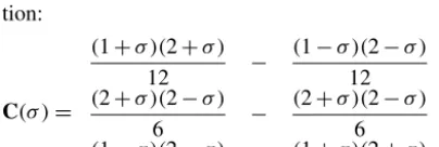
C(σ )=
(1+σ )(2+σ )
12 −
(1−σ )(2−σ ) 12 (2+σ )(2−σ )
6 −
(2+σ )(2−σ )
6 (1−σ )(2−σ )
12 −
(1+σ )(2+σ )
12 ,
(2)
whereσ is the local dip and the filtering is accomplished by convolving Eq. (2) with the GPR image.
Our goal is to suppress continuous reflections that have small dips (such as snow layering and the ground surface)
compared to the steeply dipping diffraction limbs. To esti-mate local dips, we make an initial guessσ0for the dip and
solve the set of equations
C0(σ 0)d
εD
1σ =
−C(σ0)d
0
(3)
for1σ. Here,C(σ )denotes the convolution of the filter with the data (d),C0(σ )is the derivative of the filter with respect toσ(C0(σ )dis a diagonal matrix),Dis the gradient operator, andεis a weighting parameter that controls the smoothness of the estimated dip field. Imposing smoothness constraints on the dip field estimate ensures stability in the solution and helps target the reflections in the image, since they generally show higher amplitudes and are more laterally continuous than the diffractions we seek to preserve. The estimated dip field is then used to filter the data.
2.4 Migration
Migration is the process that moves reflected and diffracted energy in a seismic or GPR record to its true location in the subsurface (i.e., Claerbout, 1985). The quality of the migra-tion process depends on the accuracy of the velocity esti-mate. When the correct migration velocity is chosen, diffrac-tion hyperbolas will collapse to a compact focus. With too low a velocity, the hyperbola will only be partially collapsed, while a velocity that is too high will cause the hyperbola to be mapped into a “smile”.
For the MVA analysis, we migrate the entire image through a suite of velocities (0.19–0.29 m ns−1in increments of 0.002 m ns−1) using MATGPR’s implementation of the Stolt algorithm (Stolt, 1955). The Stolt algorithm performs the migration in the frequency wave-number domain and is computationally efficient. To reduce computational time, we modified the code to perform all the migrations in one func-tion call so that the forward Fourier transform is only per-formed once.
2.5 Velocity picking
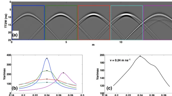
Figure 1. (a)Synthetic hyperbolas for four rectangular diffractors with lateral dimensions of 0.1, 0.2, 0.3, and 0.4 m (from left to right) and a round diffractor with radius=0.4 m (far right; TT2W is the two-way travel time).(b)Vcurve for windows depicted in(a);V curve colors match the windows in(a).V curves for all four rectangular diffractors show peaks at 0.24 m ns−1, while the round diffractor is peaked at 0.268 m ns−1.(c)Varimax curve for the entire image showing a peak at the correct migration velocity ofv=0.24 m ns−1.
al. (2007), we use the varimax norm (V):
V = N
N
P
i=1
si4
N
P
i=1
si2
2
, (4)
wheresiis the amplitude of theith sample andNis the num-ber of samples included in the calculation.V is a measure of the “simplicity” of a signal (Wiggins, 1978). Since the sim-plest possible signal is a spike and the optimal migration ve-locity will map hyperbolas to the most compact focus, the maximum V value will correspond to the image migrated with the optimal velocity.
To assess the possibility for errors in the migration velocity analysis, we applied our workflow to a synthetic data set gen-erated from diffractors of varying size. We created five syn-thetic diffractions with a migration velocity of 0.24 m ns−1. The first four (Fig. 1a) correspond to rectangular objects at 1 m depth with horizontal dimensions of 0.1, 0.2, 0.3, and 0.4 m and thickness of 0.03 m. The fifth corresponds to a circular object with a radius of 0.4 m (close to Rf for
the 500 MHz ricker wavelet used to generate the diffrac-tions). The correspondingV curves for the windows shown in Fig. 1a are plotted in Fig. 1b. TheV curves are peaked at 0.24 m ns−1for all of the rectangular diffractors, with flatter (less well-resolved) peaks as the horizontal dimension of the diffracting object increases, suggesting a larger uncertainty in the velocity estimate. The peakV value for the circular diffractor is at 0.268 m ns−1, indicating that curved objects with lateral dimensions close to the size of the Fresnel zone may continue to focus at velocities higher than their true
ve-locity. Finally, Fig. 1c shows theV curve for the entire im-age, which peaked at the correct velocity of 0.24 m ns−1. This analysis suggests that the peakVvalue will correspond to the correct velocity if the majority of the diffractions correspond to objects with a radius less thanRf.
We choose to compute V in sliding windows that span the entire time section and have a user-defined width. Com-putingV in this way allows us to incorporate many diffrac-tion events and maximize the likelihood that the bulk of the diffractions satisfy the point diffractor assumption. More-over, sliding windows offer the potential to capture lateral variability in snow density. After computingV for the entire data set, we choose the maximumV value in each window to get an estimate of the migration velocity. Noise in the filtered image, large diffracting objects, or a lack of diffractions may cause the peak of theV curve to correspond to an incorrect velocity. To reduce the influence of erroneous velocity picks, we smooth the picks in the lateral direction with a boxcar averaging filter the same width as the sliding window.
Figure 2.Justification for uncertainty estimates. A synthetic hyperbola that is obviously under-migrated(a), migrated at indistinguishable velocities(b–d), and obviously over-migrated(e).(f)The corresponding varimax curve for(a)–(e)showing a peak at the true migration velocity (0.24 m ns−1), the shaded area under the curve corresponds to velocities in(b)–(d)and represents varimax values that are 95 % of the maximum. Panels(g)–(l)show the same for a section of field data extracted from Line 1.
2.6 Dix equation
The migration velocity is the RMS velocity of all of the ma-terial between the GPR antenna and the diffractor. When the GPR antenna is in contact with the snow and the diffractor is located at the base of the snow, we interpret the migration ve-locity to be the average veve-locity of the snow across the width of the diffraction hyperbola. When the GPR unit is mounted on the front of the snowmobile, the signal must pass through the air between the antenna and the snow surface so that the migration velocity is higher than that of the snow. To find the snow velocity from these data, we use the Dix equation (Dix, 1955):
Vsnow=
s
Vmig2 tsoil−Vair2tsnow
tsoil−tsnow
, (5)
where velocity subscripts refer to the migration velocity, the velocity in air, and the velocity within the snowpack and time subscripts refer to the two-way travel times of the snow sur-face and soil sursur-face reflections.
The Dix equation contains two important assumptions. First, the velocity of the snow must be approximately con-stant over the width of the hyperbola and, second, the half-width of the hyperbola should be small compared to the depth of the diffractor (xz). The diffractions in our data sets are approximately 4 to 5 m wide; thus, we assume that any lateral variations in snow density occur on a larger scale than this. If the second assumption is not valid, then the Dix velocity will be higher than the true velocity, resulting in a density estimate that is too low. The snow depths in our data range from∼1–2 m, which is comparable to the half-width of the hyperbolas.
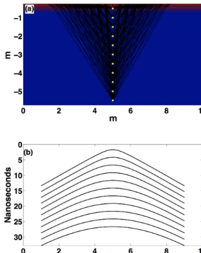
Figure 3. Ray paths and travel times for point diffractors.(a)A value of 0.5 m of air overlying a 230 m ns−1snowpack with point diffractors buried at 0.5 m intervals.(b)Two-way travel times for each of the diffractors showing the characteristic hyperbolic shape.
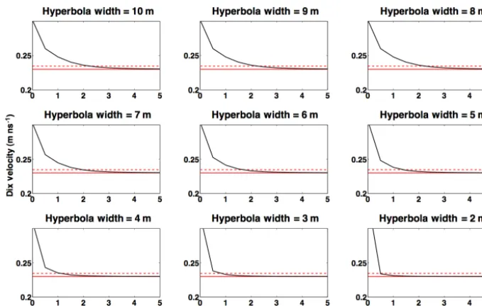
the travel-time data and successively reducing the widths of the hyperbolas from 10 to 2 m in 1 m increments. Using the Dix equation, we obtained estimates of the snow velocity as a function of diffractor depth and hyperbola width (Fig. 4). The velocity estimates made with the Dix equation approach the true velocity as the diffractor depth increases and the hy-perbola width decreases. For hyhy-perbolas that are 4–5 m wide (the average width that we observe in our data), the Dix ve-locity is within 2 % of the true veve-locity when the diffractors are about 1.5 m deep, 5 % when the diffractors are about 1 m deep, and 10 % or greater when the diffractors are 0.5 m deep. We conclude that the use of the Dix equation is justified for diffractors buried deeper than 1.5 m beneath the snow sur-face.
Although the results of this analysis are only valid for travel-time modeling, thexzassumption may be less se-vere for migration focusing analysis. Diffraction amplitudes decrease with increasing horizontal distance from the diffrac-tor location; thus, the traces closest to the diffracdiffrac-tor have the greatest contribution to the final image, suggesting that the Dix equation may give adequate results for diffractors that are less than 1.5 m deep when velocities are estimated from MVA (we test this with our synthetic data set in Sect. 3.1).
To propagate our velocity uncertainty estimates through the Dix equation, we assign an uncertainty of 0.2 ns to our travel-time observations and use Eq. (5) along with our
ve-locity uncertainty estimates to compute upper and lower bounds on the snow velocity.
2.7 Estimating SWE
To estimate SWE from the radar data, we need to know the depth of the snow and the snow density (SWE=zsnowρsnow).
The depth can be found by picking the two-way travel time of the ground reflection and, if applicable, the snow surface reflection and then using the velocity estimate to convert time to depth. Using Eq. (1), we convert radar velocity to the di-electric constant (v=c/
√
κ0)and estimate the density of dry
snow with the following empirical relationship (Tiuri et al., 1984):
κ0d=1+1.7ρ+0.7ρ2, (6)
whereκ0dis the dielectric constant andρis the density of dry
snow.
In this paper, we are primarily concerned with measur-ing radar velocities and we assume that our data measure the properties of dry snow. The dry snow assumption can be tested from the data by analyzing the attenuation proper-ties of the snowpack (Bradford et al., 2009). Because the real part of the dielectric constant for water (∼80) is much larger than that of snow (∼1.5–2) and the imaginary part, which de-scribes the attenuation of the signal, is non-negligible (Brad-ford at al., 2009), the radar signal will travel at a slower velocity and attenuate more rapidly when liquid water is present in the snow. The attenuation coefficient for radar waves in water is frequency dependent (i.e., Turner and Sig-gins, 1994), with the higher frequencies attenuating more rapidly that the lower frequencies because they go through more cycles per distance traveled.
To test the dry snow assumption, we compare the fre-quency content of the ground reflection to a reference event (the direct arrival for ski-pulled data and the snow surface reflection for the snowmobile-collected data). We calculate the maximum local instantaneous frequency (Fomel, 2007) within a time window surrounding the event of interest and then average this value across all of the traces in the GPR im-age. The standard deviation provides an estimate of the mea-surement uncertainty. We note that at 500 MHz a small shift in frequencies results in a non-negligible volumetric water content.
3 Data and results
Figure 4.Dix velocities for point diffractors as a function of depth for different hyperbola widths. The true interval velocity is 0.230 m ns−1 (red line) and the Dix velocities are shown as black lines. The red dashed line is at 0.234 m ns−1, which is 2 % greater than the true velocity.
Table 2.Summary of GPR field data and comparison to manual measurements.
GPR predictions at pit Error compared to pit/probe
GPR Collection Acquisition Pit/ Depth ρ SWE Depth ρ SWE
profile date mode probe pred. (m) (kg m−3) (m)
Line 1 25 Feb 15 Ski Pit 1 1.29±0.06 288±50 0.37±0.07 2.6 % 5.5 % 8.0 %
Line 21 25 Feb 15 Ski Pit 2 1.59±0.04 294±40 0.46± 0.03 0.1 % 6.0 % 6.0 %
Line 31 25 Feb 15 Snowmobile Pit 2 1.10±0.05 354±65 0.39±0.06 230.0 % 13 % 221 %
Line 4 11 Mar 15 Snowmobile Pit 3 1.50±0.08 389±92 0.53±0.09 6.0 % 3 % 2.0 %
Pit 4 1.91±0.12 394±97 0.69±0.13 6.0 % 10 % 6.1 %
Probes 3RMSE=0.13 m
(9 %)
Line 51 17 Mar 15 Snowmobile Probes NA NA NA 3RMSE=0.38 m NA NA
(18 %)
Line 61 17 Mar 15 Snowmobile Probes NA NA NA 3RMSE=0.19 m NA NA
(11 %)
1Lines 2, 3, 5, and 6 are described in the Supplement.2Line 3 was located 1.5 m off of Pit 2, disagreement between depth and SWE measurements at this site reflect
lateral variations in snow depth.3RMSE percentages are calculated relative to the mean observed depth along each profile.
3.1 Synthetic test
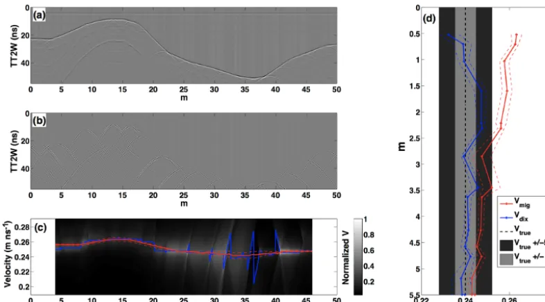
As a first test on the reliability of migration focusing analysis for reconstructing radar velocities, we performed the analy-sis on a synthetic data set generated with REFLEX software. The synthetic data set was generated using a 500 MHz Kuep-per wavelet sampled at 0.0332 ns and traces are 0.01 m apart. The synthetic model is 50 m long and consists of a 0.5 m thick layer of air overlying a 0.24 m ns−1layer of snow (cor-responding to a density of 0.29 kg cm−3) with depths that range from 0.5 to 5.7 m. Beneath the snow is a 0.10 m ns−1 layer representative of soil. Along the snow–soil interface
there are 16 diffractors buried at depths ranging from 0.5 to 5.7 m. The purpose of this data set (Fig. 5a) was to test the performance of the Dix equation on velocities estimated from the MVA analysis and, since the migration velocity changes as a function of snow depth, to see if we can resolve lateral variations in velocity.
Figure 5.Synthetic data set and velocity picking.(a)Synthetic data before filtering.(b)After PWD filtering.(c)Varimax norm for sliding window 8 m wide.(d)Velocities from synthetic data set as a function of diffractor depth. The solid blue line shows measured migration velocities; dashed blue lines show uncertainty bounds. The solid red line shows velocities computed with the Dix equation; dashed red lines show uncertainty bounds. The solid black line shows the true velocity (0.24 m ns−1). The light gray region indicates where velocities are within 2 % of the true velocity, and the dark gray region shows where velocities are with 5 % of the true velocity.
to the velocity of the snow layer (Fig. 5d). The average of all snow velocity measurements is 0.241 m ns−1with a standard deviation of 0.002 m ns−1.
There is no systematic relationship between the veloci-ties recovered and the depth of the diffractor (Fig. 5d). The shallowest diffractor was at∼0.5 m depth and the recovered velocity was 0.232 m ns−1. The greatest differences between recovered and true velocities were for diffractors at depths of 0.5, 1.6, 2.2, and 2.3 m. Here the recovered velocities were 0.232, 0.247, 0.247, and 0.248 m ns−1. The shallowest ob-servation underestimates the true velocity, which is the op-posite of the effect predicted by our travel-time modeling (Sect. 2.6, Fig. 4). The observations for diffractors between 1.5 and 2.3 m all overestimate the true velocity by approxi-mately the same amount. We conclude that the Dix equation is appropriate for snow depths of 0.5 m and greater.
Although the snow in this synthetic model has a constant velocity, the migration velocity changes as a function of the snow depth due to the changing proportions of air and snow in the total travel path. Where the snow is shallow, the ve-locities are highest and, where the snow is deep, the veloc-ities are low. That the method is capable of resolving lat-eral velocity variations in this synthetic example is evident in Fig. 5c, where the picked velocities are negatively correlated with snow depth.
3.2 Ski-pulled GPR data
We collected two GPR profiles in the ski-pulled configura-tion on 25 February 2015, in below-freezing condiconfigura-tions. A representative line, Line 1 (Fig. 6), is 74 m long and shows an abundance of diffractions along the snow–ground interface, likely a result of small boulders, and a few isolated diffrac-tions within the snowpack, most likely small trees, bushes, or logs. After interpolation to equal spacing, trace spacing was 0.0362 m. Since the antenna was coupled to the snow, we compare the average frequency of the direct wave to that of the soil reflection to determine whether there is any liq-uid water present in the snowpack. The average frequency of the direct arrival for every trace in the image along Line 1 is 410 MHz with a standard deviation of 10 MHz, and the aver-age frequency of the soil reflection across the whole line is 457 MHz with a standard deviation of 42 MHz. The soil re-flection appears to have a higher-frequency content than the reference frequency, perhaps due to thin-layer “tuning” ef-fects. Since we do not observe a decrease in frequency with travel time, we infer that there was no liquid water present in the snow on this day.
uncer-Figure 6. (a)Raw GPR data for Line 1,(b)GPR data after PWD filtering,(c)diffractions migrated at the mean velocity (0.245 m ns−1) for the entire line, and(d)normalized varimax curves for a 10 m wide sliding window. The blue curve shows the peak value for every curve; the red line is smoothed with a 10 m wide box car averaging filter.
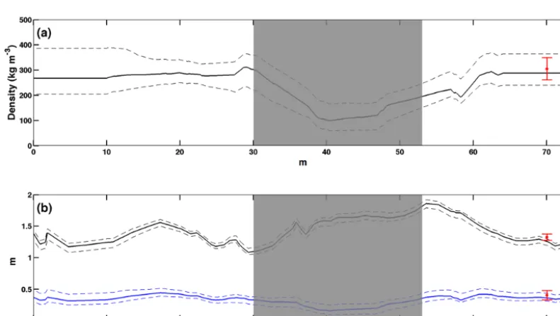
Figure 7.Line 1 results:(a)density,(b)snow depth (black line), and SWE (blue line) estimates from the GPR data; snow pit data are shown in red. Grayed out region corresponds to areas where velocity picks are unreliable.
tainty of 0.01 m ns−1, corresponding to densities of 313 to 145 kg m−3. It is unlikely that the snow density is as low as 145 kg m−3, and the velocity measurements that yield such unlikely results are confined to the region betweenx∼30– 55 m. Either the diffractors along this part of the line are all too large to meet our point diffractor assumption or the noise levels in the image are higher than the signal.
Excluding the picks between x=30 and 55 m, we esti-mate snow densities between 193 and 311 kg m−3, with an average density of 274 kg m−3. Notably, the low-density esti-mates are from the part of the profile nearx=55–65 m where a prominent set of mid-snow diffractors exist. The two-way travel time to the tops of these diffractors is ∼7.414 ns, which at the observed migration velocity of 0.256 m ns−1
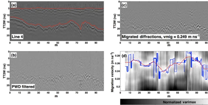
Figure 8. (a) Raw GPR data for Line 4; red lines indicate interpreted ground and snow reflection.(b) GPR data after PWD filtering, (c)diffractions migrated at the mean velocity (0.249 m ns−1) for the entire line, and(d)normalized varimax curves for a 10 m wide sliding window. The blue curve shows the peak value for every curve; the red line is smoothed with a 10 m wide box car averaging filter.
estimate of 193 kg m−3corresponds to the upper 0.95 m of
snow. Estimated snow depths, densities, and SWE along the entire profile are shown in Fig. 7.
We measured snow density and depth in Pit 1 lo-cated at 68 m along Line 1 (Fig. 7). The snow pit showed a depth of 1.33 m and an average density of 300±40 kg m−3 resulting in a SWE measurement of 0.40±0.07 m. GPR-derived estimates at the pit loca-tion are as follows: snow depth=1.28±0.06 m, den-sity=288±50 kg m−3, and SWE=0.37±0.07 m. The av-erage density of the upper 0.95 m of snow in this pit is 190 kg m−3(Fig. S1 in the Supplement), which is very close to the value estimated from the GPR data between x=55 andx=65 m.
3.3 Snowmobile-mounted GPR data
We collected four GPR profiles in the snowmobile-mounted configuration between 25 February and 17 March 2015. Here we discuss the processing of a representative profile, Line 4 (Fig. 8), which was collected on the morning of 11 March 2015 in a flat meadow just south of Wyoming Highway 130. This line is 98 m long and shows an abundance of diffractions along the snow–ground interface (Fig. 8). After interpolating to equal spacing, the trace spacing was 0.024 m.
Migration velocities on this line range from 0.237 to 0.277 m ns−1with an average uncertainty of±0.01 m ns−1. The corresponding snow velocities are 0.207 and 0.268 m ns−1. Here, the exceptionally high velocities are confined to a region betweenx=65 andx=85 m where a number of diffractions from obviously large objects are
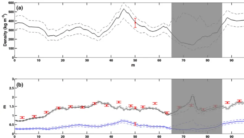
present (Fig. 8). If we exclude velocity picks from this re-gion, we get a maximum migration velocity of 0.266 m ns−1 and a maximum snow velocity of 0.251 m ns−1. Estimated snow depths range from 0.7 to 2.1 m with an average uncer-tainty of±0.1 m. Estimated snow densities range from 228 to 532 kg m−3 with an average uncertainty of ±50 kg m−3. Estimated SWE ranges from 0.25 to 0.71 m with an average uncertainty of±0.09 m.
Snow pits 3 and 4 are located at 50 and 97 m along the profile and showed average snow densities of 379±50 and 360±48 kg m−3, SWE values of 0.54±0.13 and 0.64±0.13 m, and snow depth values of 1.44±0.05 and 1.8±0.05 m, respectively. The GPR-derived depth, den-sity, and SWE estimates at 50 and 97 m were 1.50±0.08 and 1.91±0.12 m, 389±92 and 394±97 kg m−3, and
Figure 9.Line 4 results:(a)density;(b)snow depth (black line) and SWE (blue line) estimates from the GPR data; snow pit data are shown in red. Grayed out region corresponds to areas where velocity picks are unreliable.
Figure 10.Cross plots of predicted data (horizontal axis) vs. GPR estimates (vertical axis) for all data:(a)snow depths,(b)density, and (c)SWE. Black crosses represent estimates using automatically picked velocities and red crosses represent estimates using the mean velocity for each GPR profile.
4 Discussion
The primary purpose of this study is to develop an efficient processing flow for measuring GPR velocity and thus snow density SWE from common-offset data that requires a mini-mum amount of human interpretation. Common-offset GPR data are fast and easy to obtain, and velocity estimates can be made when diffractions are present. However, the com-mon methods of visually inspecting migrated images or fit-ting curves to diffraction hyperbolas are time-consuming and subject to human error. The migration velocity analysis de-scribed in this paper provides an efficient means for extract-ing velocity information from large GPR data sets. Here we discuss the accuracy and efficiency of the method as well as the level of automation.
To validate the method, we compared estimated snow den-sities, depths, and SWE to observations made in four snow
pits and to 86 probed snow depth measurements. The results are summarized in Table 2 and in Fig. 10. If we exclude the two obvious outliers (Fig. 10a), the RMS error for our depth predictions for the remaining 88 depth observations is 12 % of the mean snow depth observation. The RMS errors for snow density and SWE relative to the mean observed val-ues are 15 and 18 %. Averaging the velocities across the en-tire line (Fig. 10, red crosses) reduces the difference between predicted and observed depth values to an RMS error of 9 %, suggesting that lateral variations in snow velocity are mini-mal. Averaging the velocities across the entire line reduces the RMS errors for density and SWE to 8 and 10 %, respec-tively.
size on velocity estimates. Line 1, for example, shows four prominent diffractions between 50 and 70 m. The varimax norm has a maximum value at 0.256 m ns−1, which is the
velocity that focuses the two leftmost diffractions (Fig. 6c). The diffractions on the right are clearly not focused because they are caused by an object (most likely a log) with a ra-dius greater than the first Fresnel zone. Because the leftmost two have a higher amplitude than the others, they have the largest influence on the varimax value. Thus, although there are clearly events in the field data that have the potential to give erroneous results, our results suggest that reliable veloc-ity estimates can be achieved so long as the majorveloc-ity of the diffracted energy is related to objects that can be considered point diffractors.
One of our main goals was to produce a processing flow that allows for the rapid processing of common-offset GPR data with minimal user interaction. The two most time com-putationally expensive parts of the processes are the migra-tions and the varimax calculamigra-tions. As an example, on a 2016 MacBook Pro with a 2 GHz processor, for the∼100 m long Line 4, performing 51 migrations takes approximately 5 min, the varimax calculation takes about half as long, and the PWD filtering takes a few seconds. The most time-consuming part of the process is picking the arrival times of snow surface and ground surface reflections.
Although the processing flow is relatively efficient, it does require some user interaction. The PWD method of separat-ing continuous reflectors from diffractions treats the GPR im-age as the superposition of locally planar waves. Estimating the slope of these waves from the image requires the solution of a regularized inverse problem and the smoothness of the slope-field depends on the choice of regularization parame-ter. This is the most subjective step of the process, as it may require several attempts to find the optimal smoothness con-straints to adequately suppress reflections in the GPR image. However, for our data the majority of the diffractions are lo-cated along the ground surface and the internal structure of the snowpack shows dips that closely parallel the ground re-flection. A good first guess, and often a good final guess, for the dip field can be computed by picking the arrival times of the ground reflection. Because the ground reflection has to be interpreted to measure snow depth, this strategy can signifi-cantly reduce the processing time for each data set.
The data presented in this paper contained an abundance of diffractions located near the soil–ground interface allowing an average velocity for the entire snowpack to be obtained. These events are likely due to small-scale variations in sur-face topography, rocks, and/or vegetation along the ground surface, which may not be present in all environments. How-ever, we note that mountain watersheds free of vegetation, small undulations in surface topography, and surface rocks are probably rare. Thus, the method may be useful in many regions where a seasonal snowpack exists.
5 Conclusions
We applied the migration focusing analysis presented in Fomel et al. (2007) to the problem of estimating SWE in seasonal snow. The method was most accurate for the case when the GPR was in contact with the snow, providing GPR-derived SWE estimates within 6 % of the manual observa-tion. When the GPR was mounted on a snowmobile, the re-sults were within 12–21 % of the manual observations.
Data availability. GPR, snow density, and snow depth data are
available at https://doi.org/10.15786/M2W01X (St. Clair and Hol-brook, 2017).
The Supplement related to this article is available online at https://doi.org/10.5194/tc-11-2997-2017-supplement.
Competing interests. The authors declare that they have no conflict
of interest.
Acknowledgements. This work was funded by the US National
Science Foundation (NSF) EPSCoR program, NSF award EPS-1208909. We would like to thank Matt Provart for assisting with data collection and Mehrez Elwaseif for assistance with REFLEX software. We would also like to thank Hansruedi Maurer and another anonymous reviewer for their comments and suggestions.
Edited by: Valentina Radic
Reviewed by: Hansruedi Maurer and one anonymous referee
References
Bales, R. C., Molotch N. P., Painter, T. H., Dettinger, M. D., Rice, R., and Dozier, J.: Mountain hydrology of the western United States, Water Resour. Res., 42, W08432, https://doi.org/10.1029/2005WR004387, 2006.
Bradford, J. H.: Frequency dependent attenuation analysis of ground-penetrating radar data, Geophysics, 72, J7–J16, https://doi.org/10.1190/1.27101832007.
Bradford, J. H., Harper J. T., and Brown, J.: Complex dielectric permittivity measurements from ground-penetrating radar data to estimate snow liquid content in the pendular regime, Water Re-sour. Res., 45, W08403 https://doi.org/10.1029/2008WR007341, 2009.
Claerbout, J. F.: Imaging the Earth’s interior: Blackwell Scientific Publications, Inc., 398 pp., 1985.
Claerbout, J. F.: Earth soundings analysis: Processing versus inver-sion: Blackwell Scientific Publications, Inc., 304 pp., 1992. Conger, S. M. and McClung, D. M.: Instruments and methods
Dix, C. H.: Seismic velocities from surface measurements, Geo-physics, 20, 68–86, 1955.
Fomel, S.: Applications of plane-wave destruction filters, Geo-physics, 67, 1946–1960, 2002.
Fomel, S.: Local seismic attributes, Geophysics, 72, A29–A33, https://doi.org/10.1190/1.2437573, 2007.
Fomel, S., Landa, E., and Taner, M. T.: Poststack velocity analysis by separation and imaging of seismic diffractions, Geophysics, 72, 89–94, 2007.
Holbrook, W. S., Miller, S. N., and Provart, M. A.: Estimat-ing snow water equivalent over long mountain transects usEstimat-ing snowmobile-mounted ground-penetrating radar, Geophysics, 81, WA183–WA193, https://doi.org/10.1190/GEO-0121.1, 2016. Landa, E. and S. Keydar.: Seismic monitoring of diffraction images
for detection of local heterogeneities, Geophysics, 63, 1093– 1100, https://doi.org/10.1190/1.1444387, 1998.
Molotch, N. and Bales, R. C.: Scaling snow observations from the point to the grid element: Implications for ob-servation network design, Water Resour. Res., 41, W11421, https://doi.org/10.129/2005WR004229, 2005.
Serreze, M. C., Clark, M. P., Armstrong, R. L., McGinnis, D. A., and Pulwarty, R. S.: Characteristics of the western United States snowpack from snowpack telemetry (SNOTEL) data, Water Re-sour. Res., 35, 2145–2160, 1999.
St. Clair, J. and Holbrook, W. H.: Data for “Measuring snow wa-ter equivalent from common offset GPR records through migra-tion velocity analysis”, University of Wyoming Research Data Repository, https://doi.org/10.15786/M2W01X, 2017.
Stolt, R. H.: Migration by Fourier Transform, Geophysics, 43, 23– 48, 1978.
Tiuri, M. E., Sihvola, A. H., Nyfors, E. G., and Hallikaiken, M. T.: The complex dielectric constant of snow at microwave frequen-cies, IEEE J. Oceanic Eng., 9, 377-382, 1984.
Turner, G., and Siggins, A. F.: Constant Q attenuation of subsurface radar pulses, Geophysics, 59, 1192–1200, https://doi.org/10.1190/1.443677, 1994.
Tzanis, A.: MATGPR: A freeware MATLAB package for the anal-ysis of common-offset GPR data, Geophysical Research Ab-stracts, 8, 09488, 2006.