www.the-cryosphere.net/10/2113/2016/ doi:10.5194/tc-10-2113-2016
© Author(s) 2016. CC Attribution 3.0 License.
Retrieving the characteristics of slab ice covering snow
by remote sensing
François Andrieu1, Frédéric Schmidt1, Bernard Schmitt2,3, Sylvain Douté2,3, and Olivier Brissaud2,3 1GEOPS, Univ. Paris-Sud, CNRS, Université Paris-Saclay, Rue du Belvédère, Bât. 504-509, 91405 Orsay, France 2Univ. Grenoble Alpes, IPAG, 38000 Grenoble, France
3CNRS, IPAG, 38000 Grenoble, France
Correspondence to:F. Andrieu ([email protected])
Received: 15 July 2015 – Published in The Cryosphere Discuss.: 29 September 2015 Revised: 3 July 2016 – Accepted: 26 July 2016 – Published: 15 September 2016
Abstract. We present an effort to validate a previously de-veloped radiative transfer model, and an innovative Bayesian inversion method designed to retrieve the properties of slab-ice-covered surfaces. This retrieval method is adapted to satellite data, and is able to provide uncertainties on the re-sults of the inversions. We focused on surfaces composed of a pure slab of water ice covering an optically thick layer of snow in this study. We sought to retrieve the roughness of the ice–air interface, the thickness of the slab layer and the mean grain diameter of the underlying snow. Numerical vali-dations have been conducted on the method, and showed that if the thickness of the slab layer is above 5 mm and the noise on the signal is above 3 %, then it is not possible to invert the grain diameter of the snow. In contrast, the roughness and the thickness of the slab can be determined, even with high levels of noise up to 20 %. Experimental validations have been con-ducted on spectra collected from laboratory samples of water ice on snow using a spectro-radiogoniometer. The results are in agreement with the numerical validations, and show that a grain diameter can be correctly retrieved for low slab thick-nesses, but not for bigger ones, and that the roughness and thickness are correctly inverted in every case.
1 Introduction
Various species of ice are present throughout the solar sys-tem, from water ice and snow on Earth to nitrogen ice on Triton (Zent et al., 1989), not to forget carbon dioxide ice on Mars (Leighton and Murray, 1966). The physical properties
of the cover also have an impact on the energy balance; for example, the albedo depends on the grain size of the snow (Dozier et al., 2009; Negi and Kokhanovsky, 2011; Picard et al., 2009; Mary et al., 2013), on the roughness of the in-terface (Lhermitte et al., 2014), on the presence or lack of impurities and the physical properties of impurities (Dumont et al., 2014). The study and monitoring of theses parameters is key to constraining the energy balance of a planet.
ob-jects: CO2on Mars (Kieffer and Titus, 2001; Eluszkiewicz et al., 2005), N2 on Triton and Pluto (Zent et al., 1989; Eluszkiewicz and Moncet, 2003) and probably SO2 on Io (Eluszkiewicz and Moncet, 2003), as suggested by the very long light path lengths measured, over several centimeters to decimeters (Eluszkiewicz, 1993; Quirico et al., 1999; Douté et al, 1999, 2001). In particular, the Martian climate is mostly controlled by a seasonal CO2cycle that results in the conden-sation and sublimation of deposits constituted of a layer of nearly pure CO2ice up to 1 m thick, possibly contaminated with H2O ice and regolith dust (Leighton and Murray, 1966; Eluszkiewicz et al., 2005). The monitoring of the evolution of these deposits’ composition would bring key pieces of in-formation on the water ice cycle on Mars and on the dust transport to the surface.
Compact slabs have very different radiative properties from closely packed granular media, and radiative transfer models have been developed to study their characteristics (e.g., Mullen and Warren, 1988; Jin et al., 1994; Perovich, 1996; Jin et al., 2006) in the case of sea or lake ice. We de-veloped an approximated model (Andrieu et al., 2015d) that has the capability of being able to model a layer of ice cov-ering a surface with radically different optical properties, for instance a different refractive index, unlike its predecessors. It was originally designed for the study of Martian seasonal ice deposits, using massive spectro-imaging datasets, such as the OMEGA (Bibring et al., 2004) or CRISM (Murchie et al., 2007) datasets. For this purpose, it is semi-analytic and implemented to optimize the computation time. How-ever, the algorithm was built to be adaptable to any other spectroscopic data, from terrestrial water ice laboratory mea-surements, as is the case of this work, to the study of SO2 ice on Io or N2ice on Pluto using the NIMS (Carlson et al., 1992) and RALPH (Reuter et al., 2009) datasets respectively. In the present article, we test the accuracy of this approx-imated model on laboratory spectroscopic measurements of the bidirectional reflectance distribution function (BRDF) of pure water ice on top of snow. At the same time, we present an innovative Bayesian inversion method that was developed to retrieve the properties of solar system compact ice using satellite spectro-imaging data. In this paper, the term “inver-sion” is used and means “solving the inverse problem”. The slabs that are studied contain no impurity, and the surface properties we seek to retrieve are the thickness of the ice, the roughness of the ice–air interface and the grain diameter of the underlying snow. The main goals of this work are (i) to test the ability of the model to reproduce reality and (ii) to propose an inversion framework able to retrieve surface ice properties, including uncertainties, in order to demonstrate the applicability of the approach to satellite data.
We present a set of spectro-goniometric measurements of different water ice samples put on top of snow using the spectro-radiogoniometer described in Brissaud et al. (2004). Three kind of experiments were conducted. First, the BRDF of only one snow layer was measured, and then it was
mea-sured again after adding a slab ice layer at the top. The objec-tive was to test the effect of an ice layer at the top of the snow on the directivity of the surface. Second, the specular lobe was closely investigated, at high angular resolution, at the wavelength of 1.5 µm, where ice behaves as a very absorb-ing media. Finally, the bidirectional reflectance was sampled at various geometries on 61 wavelengths ranging from 0.8 to 2.0 µm. In order to validate the model, we did qualitative tests to demonstrate the relative isotropization of the flux. We also conducted quantitative assessments by using a Bayesian inversion method in order to estimate the sample thickness, the surface roughness and the snow grain diameter from the radiative measurements only. A comparison between the re-trieved parameters and the direct independent measurements allowed us to validate the model.
The inversion algorithm that is tested is based on lookup tables (LUTs) that minimize the computation time of the direct model. The solution is formulated as a probability density function, using Bayesian formalism. This strategy is very useful for analyzing hyperspectral images. The thick-ness of ice estimated from the inversion is compared to real direct measurements. In addition, the power distribution in the specular lobe, which is determined by the roughness of the surface, is adjusted to demonstrate that the model is able to reasonably fit the data with a consistent roughness value.
2 Description of the model
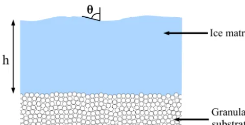
The model by Andrieu et al. (2015d) is inspired by an exist-ing one described in Hapke (1981) and Douté and Schmitt (1998), which simulates the bidirectional reflectance of strat-ified granular media. It has been adapted to compact slabs, contaminated with pseudo-spherical inclusions, and a rough top interface. In the context of this work, we suppose a layer of pure slab ice, overlaying an optically thick layer of gran-ular ice, as described in Fig. 1. The roughness of the first in-terface is described using the probability density function of orientations of slopes defined in Hapke (1984). This distribu-tion of orientadistribu-tions is fully described by a parameterθ¯, which can be interpreted as a mean slope parameter at the surface, in the case of small angles. The ice matrix is described using its optical constants and its thickness.
Figure 1. Scheme of the surface representation in the radiative transfer model applied to the laboratory measurements.hrepresents the slab thickness andθ¯represents the mean slope parameter used to describe the surface roughness.
D Ice slab
F F
ef Wf z
e i
R
R
specspecF F
Granular substrate
T T00''
rS R0
rS
...
R
DiffR
R00'' T0 T0
R0
Figure 2.Illustration of the radiative transfer in the surface medium. Anisotropic transits are represented in red.F is the incident radia-tion flux,RspecandRDiffare the specular and diffuse contributions to the reflectance of the surface respectively,rsis the Lambertian re-flectance of the granular substrate andR0andT0are the total reflec-tion and transmission factors of the slab layer respectively. A prime indicates an anisotropic transit. The reflection and transmission fac-tors are different in the cases of isotropic or anisotropic conditions. The granular and slab layers are artificially separated in this figure to help the understanding of the coupling between the two layers. Top: illustration of the reflections and transmission at the first in-terface, used in the calculations ofRspecand the determination of the amount of energy injected into the surface.zis the normal to the surface,Wfthe local normal to a facet,iandeare the incidence and emergence angles respectively andefis the local emergence angle for a facet. Each different orientation of a facet will lead to a dif-ferent transit length in the slab. A more detailed description can be found in Andrieu et al. (2015d).
at a given incidence. This gives the total amount of energy transmitted into the system constituted of the contaminated slab and the substrate. The diffuse contribution is then esti-mated through solving the radiative transfer equation inside this system under various hypotheses. The following con-siderations are made. (i) The first transit through the slab is anisotropic due to the collimated radiation from the source, and due to there being an isotropization at the second rough interface (i.e., when the radiation reaches the semi-infinite substrate). For the refraction and the internal reflection, ev-ery following transit is considered isotropic. (ii) The geomet-rical optics is valid. The reflection and transmission factors of the layers are obtained using an analytical estimation of the Fresnel coefficients described in Chandrasekhar (1960) and Douté and Schmitt (1998), as well as a simple statistical approach, detailed in Andrieu et al. (2015d). The contribu-tion of the semi-infinite substrate is described by its single-scattering albedo. Finally, as the slab layer is under a col-limated radiation from the light source, and under a diffuse radiation from the granular substrate, the resulting total bidi-rectional reflectance is computed using adding–doubling for-mulas (Stamnes et al., 1988; Douté and Schmitt, 1998; Van de Hulst, 2012).
In this work, the radiative transfer model described in An-drieu et al. (2015d) is used to simulate the reflectance fac-tor spectrum of a pure slab of water ice covering a layer of snow, as represented in Fig. 1. This spectrum may vary in terms of three parameters: (i) the roughnessθ¯of the slab ice surface, which characterizes the power distribution in the specular lobe; (ii) the thicknesshof the slab ice layer, which determines the absorption in the ice layer and (iii) the grain diametersof the snow, which determines the absorption in the snow.
3 Data
3.1 Spectro-radiogoniometer
The bidirectional reflectance spectra were measured using the spectro-radiogoniometer from Institut de Planétologie et d’Astrophysique de Grenoble, fully described in Brissaud et al. (2004). We collected spectra in the near-infrared spec-trum at incidences ranging from 40 to 60◦, emergence angles from 0 to 50◦and azimuth angles from 0 to 180◦. The sample is illuminated with a 200 mm large monochromatic beam (di-vergence<1◦), and the near-infrared spectrum covering the
result-ing in a notable angular drift on the emergence measured up to 1◦.
3.2 Ice BRDF measurements
The ice samples were obtained by sawing artificial columnar water ice into circular sections 20 cm in diameter. These sec-tions were put on top of an optically thick layer of compacted snow that was collected in Arselle, in the French Alps. The spectral measurements were conducted in a cold chamber at 263 K. However, the ice and the snow were unstable in the measurement’s environment, due to the dryness of the cham-ber’s atmosphere. The grain size of the snow showed evo-lution, and the thickness of a given slab showed a decrease of 0.343 mm day−1. Each sample needed an acquisition time of 10 h. For each measurement, the ice slab was sliced, and its thickness was measured in five different locations. It was then set on top of the snow sample, and this system was put into rotation in the spectro-radiogoniometer for the measure-ment. The sample completes a full rotation (10 s) during the measurement of the reflectance at one wavelength and one geometry. As the surface is not perfectly planar, the measured thickness is not constant. This results in an 2σ standard de-viation in the measurement of the thickness that ranges from 0.54 to 2.7 mm in our study, depending on the sample. 3.2.1 Specular contribution
The specular reflectance was measured on a slab sample on top of Arselle snow, 12.51 mm thick. This sample is de-scribed as sample 3 in the next paragraph. The illumination was at an incidence angle of 50◦, and 63 different emergent geometries were sampled, ranging from 45 to 55◦ in emer-gence and from 170 to 180◦in azimuth. The specular lobe is sampled every 1◦in emergence and azimuth, and within 47 and 53◦in emergence and 175 and 180◦in azimuth.
3.2.2 Ice on snow diffuse reflectance spectra
The diffuse contribution was measured on three samples of different slab thickness. The three thicknesses were mea-sured on different locations of the samples with a caliper be-fore doing the spectro-goniometric measurement, resulting in
h1=1.42±0.47 mm,h2=7.45±0.84 mm andh3=12.51± 2.7 mm, respectively, for samples 1, 2 and 3, with errors at 2σ. Sixty-one wavelengths were sampled ranging from 0.8 to 2.0 µm. Spectra were collected on 39 different points of the BRDF for the incidence, emergence and azimuth angles:
40,50,60◦
, [0,10,20] and
0,45,90,140,160,180◦
, re-spectively. This set of angles results in only 39 different geometries because the azimuthal angle is not defined for a nadir emergence.
Diffuse reflectance spectra of natural snow only were also measured before putting a slab on top of the snow. The ob-jective was to estimate the effect of a slab layer on the BRDF.
4 Method
We designed an inversion method aimed at massive data analysis. This method consists of two steps: first, the gen-eration of a synthetic database that is representative of the variability in the model, and then the comparison with actual data. To generate the synthetic database, we used optical con-stants for water ice at 270 K. The 7 K difference between the actual temperature of the room and the temperature assumed for the optical constants has a negligible effect. We combined the datasets of Warren and Brandt (2008) and Schmitt et al. (1998), making the junction at 1 µm, the former set for the shorter wavelengths and the latter for the wavelengths larger than 1 µm.
In order to validate the model on the specular reflection from the slab, we chose to use the reflectance at 1.5 µm, where the ice is very absorptive. Figures 7 and 8 clearly demonstrate that there is a negligible diffuse contribution in geometry outside the specular lobe from the sample with a 12.51 mm thick pure slab. Thus, the roughness parameter
¯
θis the only one impacting the reflectance in the model. We chose to invert this parameter first and validate the specular contribution.
We then focused on the validation in the spectral domain, for the diffuse contribution. We used the estimation of the roughness parameterθ¯obtained earlier and the spectral data in order to estimate the slab thickness and the grain size of the snow substrate. To do this, we assumed that the roughness was not changing significantly enough to have a notable im-pact on diffuse reflectance from one sample to another. This assumption is justified by the fact that the different columnar ice samples were made the same way, as flat as possible, and the low value ofθ¯retrieved as discussed in the next section. It is confirmed by the results of Sect. 4.2, which suggest a very low roughness, as expected. Such low roughness parameters have a negligible influence on the amount of energy injected into the surface.
4.1 Inversion strategy
The inversion consists in estimating the model parametersm
(i.e., the slab thickness, the roughness parameter, the snow grain diameter) from the modelsF(m)) (the reflectance sim-ulations) that best reproduce the datad (the reflectance ob-servations). Looking for these parameters sets is called the inverse problem. Tarantola and Valette (1982) showed that this inverse problem can be mathematically solved by consid-ering each quantity as a probability density function (PDF). In nonlinear direct problems, the solution may not be ana-lytically approached. Nevertheless, it is possible to sample the solutions’ PDF with a Monte Carlo approach as shown in Mosegaard and Tarantola (1995), but this solution is very time-consuming.
as-sumed to be anN-dimension multivariate Gaussian distribu-tion G(dmes,C), centered ondmes with a covariance matrix C. The measurements at any given wavelength/geometry are supposed to be independent from each other, as each mea-surement of one wavelength, at one geometry is done indi-vidually. The matrixCis thus assumed to be diagonal and its diagonal elementsCiiareσ12, . . ., σN2, withσibeing the stan-dard deviations corresponding to the uncertainties of each measurement. The a priori information on model parame-tersρM(m)in the parameters spaceMis independent of the data and corresponds to the state of null informationµD(d) if no information is available on the parameters. We consider a uniform PDF in their definition spaceM. The a posteriori PDF in the model space σM(m)as defined by Bayes’ theo-rem (Tarantola and Valette, 1982) is
σM(m)=kρM(m)L(m), (1)
wherekis a constant andL(m)is the likelihood function,
L(m)=
Z
D
ρD(d) θ (d|m) µD(d)
dd, (2)
whereθ (d|m)is the theoretical relationship of the PDF for
d given m. We do not consider errors of the model itself, soθ (d|m)=δ(F(m))is also noteddsimfor simulated data. Therefore, the likelihood is simplified into
L(m)=G(F(m)−dmes,C), (3)
and in the case of uniform a priori information ρM(m), the a posteriori PDF is
σM(m)=kL(m). (4)
This expression is explicitly
σM(m)=k·exp
−1 2×
t
(F(m)−dmes)C
−1
(F(m)−dmes)
,
(5) where the superscripttis the transpose operator that applies to(F(m)−dmes). The factorkis adjusted to normalize the PDF. The mean value of the estimated parameter can be com-puted by
hmi =
Z
M
m·σM(m)dm, (6)
and the standard deviation,
σhmi=
Z
M
(m− ¯m)2·σM(m)dm. (7)
In order to speed up the inversion strategy but keep the ad-vantage of the Bayesian approach, we choose to sample the
parameter spaceM with regular and reasonably fine steps, notedi. The likelihood for each element is
L(i)=exp
−1 2×
t(d
sim(i)−dmes)C
−1
(dsim(i)−dmes)
. (8) The derivation of the a posteriori PDF with such formalism for specular lobe inversion and for spectral inversion is ex-plained in the next sections.
4.2 Specular lobe
To study the specular lobe, we have to consider the whole angular sampling of the spot as a single data measurement. Similar to the “pixel” (contraction ofpicture element), we choose to define the “angel” (contraction ofangular element) as a single element in a gridded angular domain. Interest-ingly, angel also refers to a supernatural being represented in various forms of glowing light. A single angel measurement could not well constrain the model, even at different wave-lengths. Instead, a full sampling around the specular lobe should be enough, even at one single wavelength. We chose a wavelength where the diffuse contribution was negligible in order to simplify the inversion strategy. We chose to fo-cus on the 1.5 µm wavelength, as we measured a penetration depth lower than 1 mm and thus much lower than the thick-ness of the used sample for this channel. We first generated a synthetic database (lookup table), using the direct radiative transfer model. We simulated spectra in the same geometri-cal conditions, for a 12.5 mm thick ice layer over a granular ice substrate constituted of 1000 µm wide grains. These two last parameters are not important since the absorption is so high in ice, such that the main contribution is from the spec-ular reflection, and the diffuse contribution is negligible (the penetration depth inside a water ice slab at the 1.5 µm wave-length is lower than 1 mm).
The sampling of the parameter space, i.e., the lookup table, must correctly represent the variability of the model accord-ing to its parameters. For this study, we sampled the rough-ness parameter from 0.1 to 5◦ with a constant step dθ¯= 0.01◦. We used a likelihood functionL defined in Eq. (8), wheredsim anddmesarengeom-element vectors, withngeom the number of angels (63 in this study). They respectively represent the simulated and measured reflectance at a given wavelength in every geometry.Cis angeom×ngeommatrix. It represents the uncertainties of the data. In this case, we considered each wavelength independently, thus generating a diagonal matrix, containing the level of errors given by the technical data of the instrument described by Brissaud et al. (2004). It corresponds at this wavelength to 2 % of the sig-nal. The roughness parameterθ¯ returned by the inversion is described by its normalized PDF:
P¯
θ (i) = L (i)d ¯
θ
P
jL (j )dθ¯
= L (i)
P
jL (j )
The value θ (i)¯ in the database with the highest probability (maximum likelihood) corresponds to the sampling step that is closest to the maximum of the a posteriori PDF. If the PDF is close to a Gaussian, then the solution to the inverse prob-lem can be estimated by its mean,
¯
θ=
P
iθ (i) L (i)¯
P
iL (i)
, (10)
and associated standard deviations,
σhθ¯i =
v u u t
P
i θ (i)¯ −
¯
θ2L (i)
P
iL (i)
. (11)
We give error bars on the results that correspond to two stan-dard deviations, and thus a returned value forθ¯that is
¯
θr=
¯
θ±2σhθ¯i. (12)
4.3 Diffuse spectra
When out of the specular lobe, the radiation is controlled by the complex transfer through the media (slab ice and bottom snow). The experimental samples were made of pure water slab ice, without impurity. We generated the lookup table for every measurement geometry at very high spectral resolu-tion (4.10−2nm), and then downsampled it at the resolution of the instrument (2 nm). We sampled the 17 085 combina-tions of two parameters for the 39 different geometries: p1, the thickness of the slab from 0 to 20 mm (notedi= [1,201]) every 0.1 mm (noted dp1), andp2, the grain size of the gran-ular substrate from 2 to 25 µm every 1 µm and from 25 to 1500 µm every 25 µm (notedj= [1,85]and the correspond-ing dp2(j )). The parameters’ space is thus irregularly paved with dp(i, j )=dp1.dp2(j ).
For the inversion, we used the same method as previously described, with a likelihood functionLthat is written as in Eq. (8). Two different strategies were adopted. First, we in-verted each spectrum independently. Thirty-nine geometries were sampled (described in Sect. 3.2), and thus we conducted 39 inversions for each sample. This time dsimanddmes are thus respectively the simulated and measured spectra. There-fore dsim anddmes arenb-element vectors, wherenb is the number of bands (61 in this study) andCis anb×nbmatrix. As previously done (see Sect. 4.2), we considered each wave-length independently, thus generating a diagonal matrix, con-taining the level of errors given by the technical data of the instrument given by Brissaud et al. (2004). The error is a per-centage of the measurement, and thusCis different for every inversion.
Secondly, we inverted the BRDF as a whole, for each sample. For this method, dsim anddmes are the simulated and measured BRDF respectively and are thus nb×n geom-element vectors (2379 in this study), wherenbis the number of bands (61 in this study) andngeom is the number of ge-ometries (39 in this study) sampled.Cis a nb×ngeom
×
nb×ngeom diagonal matrix, containing the errors of the data. We represent the results the same way as previously, but there are two parameters to inverse. For the sake of readabil-ity, we plot the normalized marginal probability density func-tion for each parameter. We present here the general method for the inversion ofnp=2 parameters: the slab thickness and the grain size of the substrate. The PDF for the two parame-terspis described by
P{p(i, j )} = L (i, j )dp (i, j )
P
i
P
jL (i, j )dp (i, j )
. (13)
For a given parameterp1, the marginal PDF of the solution is
P{p1(i)} =
L0(i)dp1(i)
P
i
P
jL (i, j )dp (i, j )
, (14)
with L0(i)=P
jL(i, j )dp2(j ). The value p1(i) in the database with the highest probability (maximum likelihood) corresponds to the sampling step that is closest to the maxi-mum of the a posteriori PDF. The marginal PDF can be de-scribed by the mean,
hp1i =
P
ip1(i) L0(i)dp1(i)
P
i
P
jL (i, j )dp (i, j )
, (15)
and the associated standard deviation,
σhp1i=
s P
i(p1(i)− hp1i)2L0(i)dp1(i)
P
i
P
jL (i, j )dp (i, j )
. (16)
As for the roughness parameter, we give error bars on the results that correspond to two standard deviations, and thus a returned value forp1that is
p1r= hp1i ±2σhp1i. (17)
4.4 Numerical validations of the inversion method In order to numerically validate the inversion method de-scribed above, two kinds of tests were conducted. First, we applied Gaussian noise and inverted every spectrum in the synthetic spectral database. We show that with a negligible noise, the parameters are always correctly retrieved with neg-ligible uncertainties, and as the level of noise on the data increases, so do the uncertainties on the results. Secondly, we generated spectra for parameters that were not sampled in the database and tried to recover their characteristics suc-cessfully.
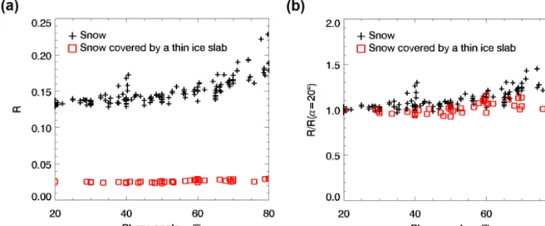
Figure 3. (a)Reflectance factor at a wavelength ofλ=1.4 µm vs. phase angle for snow only (black crosses) and the same snow but covered with a 1.42±0.27 mm water ice slab (red squares).(b)Same data but normalized by the value at a phase angleα=20◦.
centered on the correct value and the dispersion suggests an a posteriori uncertainty lower than the retrieved value. When the thickness of the slab layer increases, so does the a pos-teriori uncertainty on the estimation of the grain diameter. For a slab thickness of 5 mm (Fig. 4b), the a posteriori uncer-tainty is of the same order as the estimated value, meaning that the grain diameter cannot be retrieved. The grain diame-ter of the snow thus cannot be retrieved for slab thicknesses greater than 5 mm.
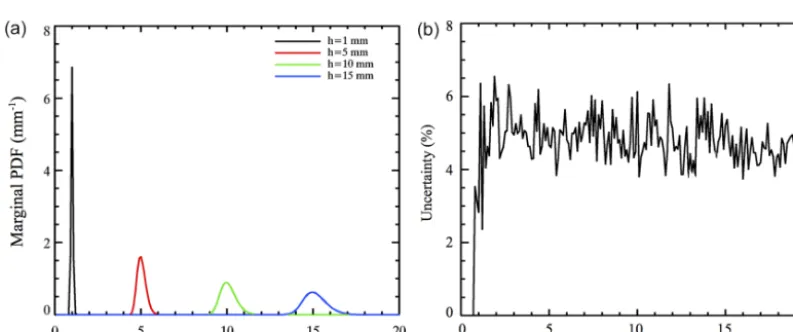
Figure 5a represents the stack of 1000 a posteriori PDFs for the thickness of the ice layer. These PDFs do not depend on the grain diameter of the snow, but only on the thickness itself and the level of noise. It shows that the thickness can be estimated, in the experimental conditions (2 % noise level), with an uncertainty of 2 % for lowest thicknesses to 5 % for highest ones. All obtained a posteriori PDFs for the thickness were very close to a Gaussian function. We were thus able to sum them up by their means and standard deviations, allow-ing us to plot, for example, the uncertainty of the thickness estimation as a function of the thickness that we want to es-timate (Fig. 5b) and of the level of noise on the data (Fig. 6). Figure 5b shows the uncertainty (at 2σ) on the estimation of the thickness of the slab layer as a function of the thickness itself, in the experimental conditions described by Brissaud et al. (2004), which means a 2 % noise level on the signal. This relative uncertainty does not depend on the thickness in the range of values tested. The low values for thicknesses below 1 mm are an effect of the discretization in the LUT: the thickness has been sampled every 0.1 mm. Below 1 mm, this sampling step is large relatively to the values itself and ranges from 10 to 100 %. The relative uncertainty that we ex-pect to be about 5 % is then no longer measurable, and the value drops to 0.
Figure 6 shows the evolution of the a posteriori uncertain-ties for the estimations of thicknesses and grain diameters as a function of the noise level. For the grain diameters, a
slab thickness of 2 mm has been used. The results show that with very low noise, i.e., lower than 0.5 %, the a posteriori uncertainties of the results are of the same order of magni-tude, even for the grain diameters. When the level of noise increases, the uncertainties of the thickness estimations in-crease in the same proportions (Fig. 6b), unlike the uncer-tainties of grain diameters (Fig. 6a) that increase drastically with the noise level. The uncertainties of the grain diameters seem to be saturated for high noises. This effect is only an edge effect due to the size of the LUT: the dispersion of the a posteriori PDFs cannot get bigger than the range of values tested.
With the level of noise at 2 % as expected for the measured spectra (Brissaud et al., 2004), a posteriori uncertainties are expected to be about 5 % on the thickness, and should be lower than 50 % for the grain diameter for low thicknesses. This means that the method should be able to retrieve thick-nesses with an uncertainty that corresponds to the level of noise, but cannot retrieve the grain diameters of the snow when the ice layer above is thicker than 5 mm.
5 Results
5.1 Impact of a slab on the BRDF
Figure 4.Normalized stacks of 1000 a posteriori PDFs for the grain diameter of the snow, when conducting the inversion on synthetic data, with added random noise. The legends indicate the values for the grain diameter used to create the synthetic data.(a)The ice layer is 1 mm thick.(b)The ice layer is 5 mm thick.
Figure 5. (a)Normalized stacks of 1000 a posteriori PDFs for the thickness of the slab ice layer, when conducting the inversion on synthetic data, with added random noise. The legends indicate the values for the thickness used to create the synthetic data.(b) The a posteriori uncertainty (at 2σ) on the thickness estimation as a function of the slab thickness.
phase angle is strongly attenuated by the addition of the ice layer. The second effect is that the radiation is more Lamber-tian than that of snow only. These data give credit to the first hypothesis of isotropization of the radiation formulated in the model (see Sect. 2). The description of the bottom granu-lar layer as Lambertian, defined only by its single-scattering albedo, may be considered simplistic, but this dataset shows that a thin coverage of slab ice, even on a very directive ma-terial such as snow, is enough to strongly flatten the BRDF. 5.2 Specular lobe: roughness retrieval
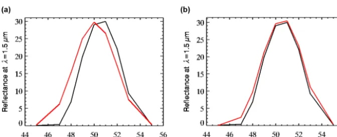
We performed the inversion taking into account 63 angel measurements, but for the sake of readability, Fig. 7 repre-sents only the reflectance in the principle plane. The shapes and the intensities in Fig. 7a are compatible, but the mea-surement and simulation are not centered at the same point.
The simulation is centered at the geometrical optics spec-ular point (emergence 50◦ and azimuth 180◦), whereas the measurement seems to be centered around an emergence of 50.5◦. This could be due to slight misadjustment of the rota-tion axis of the sample in the instrument. This kind of misad-justment is common, and can easily result in a notable shift up to 1◦of the recorded measurement geometries. We
Figure 6. (a)A posteriori uncertainties at 2σon the grain diameter as a function of the noise standard deviation, for a 2 mm thick ice layer. (b)A posteriori uncertainties at 2σon the thickness as a function of the noise standard deviation.
Figure 7. (a)Measured (black) and simulated (red) reflectance factor at 1.5 µm in the principal plane for an incidence angle of 50◦. The specular lobe measured is not centered at 50◦.(b)Measured (black) and simulated (red) reflectance factor at 1.5 µm in the principal plane for an incidence angle of 50◦. We simulated a small misadjustment of the sample, resulting in a shift of the observation of 0.5◦in emergence and 0.2◦in azimuth.
increase in the Fresnel reflection coefficient when the phase angle increases for this range of geometries. Figure 9 shows the a posteriori PDF for the parameterθ¯. The simulation cor-responding to the maximum likelihood was obtained with
¯
θ=0.43◦. The inversion method gives a result with a close to Gaussian shape atθ¯=0.424◦±0.046◦. Unfortunately, we have no direct measurement of θ¯ because the experimental determination of the roughness of a sample requires a digital terrain model (DTM) of its surface. These DTMs are mea-sured with a laser beam, and are thus very difficult to obtain for ice samples, as multiple reflections create false measures. Still, we find a low value, which is consistent with the pro-duction of slabs of columnar ice in the laboratory that are very flat, but still imperfect as described in the dataset. The average slope is compatible with a long-wavelength slope at the scale of the sample, demonstrating that the microscale was not important in our case. Indeed, for a sample that has a length L, a 1σ standard deviation on the thickness 1h
can be attributed to a general slopeϑ=arctan 1hL due to
a small error in the parallelism of the two surfaces of the slab. In the case of sample 3,L=20 cm and1h=1.35 mm result inϑ=0.39◦, which is compatible with the roughness given by the inversion. We thus think that what we see is an apparent roughness due to a small general slope on the sam-ples, and that the roughness at the surface is much lower than this value.
Figure 8.Measured and simulated reflectance factor around the specular geometry at 1.5 µm for an incidence angle of 50◦. The simulation was computed assuming the determined shift of 0.5◦in emergence and 0.2◦in azimuth.
Figure 9. The a posteriori probability density function for the roughness parameter θ¯, notedP¯
θ . The inverted value at 2σ is ¯
θ=0.424±0.046◦. The simulation corresponding with the highest likelihood is obtained forθ¯=0.43◦.
5.3 Diffuse reflectance: thickness and grain diameter retrieval
5.3.1 Example of individual geometries
To reproduce diffuse reflectance we used the results obtained with the specular measurements and assumed that the rough-ness of the samples did not change much between the ex-periments. The range of variations in roughness should be negligible in the spectral analysis. We simulated slabs over snow, with the grain diameter of the substrate and the thick-ness of the slab as free parameters. Figure 10 represents three examples of measured and simulated reflectance spectra at the maximum likelihood for three different geometries. We also represented the mismatch between these simulations and
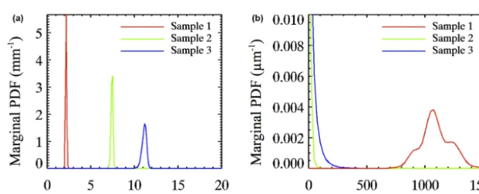
the observations. We find an agreement between the data and the model that is acceptable. Nevertheless, there seems to be a decrease in quality in the fits as the thickness increases. Fig-ure 11 shows an example of the marginal PDF for the three samples that are associated with the previous fits. The thick-ness is well constrained as the marginal a posteriori probabil-ity densprobabil-ity functions are sharp and very close to a Gaussian function. However, the grain diameter of the substrate seems to have a limited impact on the result since it is only slightly constrained. The marginal PDFs for the grain diameter of the substrate are broad, and thus the a posteriori relative uncer-tainties in the result are very high. Unfortunately, we have no reliable measurement of the grain diameter of the substrate, as it is evolving during the time of the measurements. Numer-ical tests show that the snow grain diameter is not accessible for slab thicknesses above 5 mm. The a posteriori PDFs for samples 2 and 3 are then not to be interpreted.
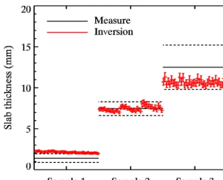
5.3.2 Results for 39 geometries
Figure 10. Reflectance factor spectra for the measure and the simulation at the maximum likelihood, and for the geometry for which maximum likelihood was highest, for each sample: at incidence 40◦, emergence 10◦and azimuth 140◦for sample 1 (thickness: 1.42 mm)(a); at incidence 40◦, emergence 20◦and azimuth 45◦for sample 2 (thickness: 7.45 mm)(b); and at incidence 60◦and emergence 0◦for sample 3 (thickness: 12.51 mm)(c). The thicknesses indicated were measured before putting the sample into the spectro-radiogoniometer, and the errors are given at 2σ. The absolute differences are shown in blue on each graph.
Figure 11.Marginal a posteriori probability density functions for(a)the thickness of the slabP{p1(i)}and(b)the grain diameter of the snow substrateP{p2(j )}for the three samples, and for the geometries described in Fig. 10.
tends to increase with incidence and decrease with azimuth. This effect disappears for large thicknesses (sample 3). 5.3.3 Full BRDF inversion
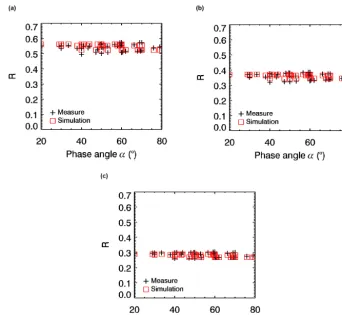
Figure 13 shows the measure and the simulation correspond-ing to the maximum likelihood at theλ=1.0 µm wavelength when conducting the inversion on the whole BRDF dataset for each sample. The relatively flat behavior of the radia-tion with the phase angle is reasonably well reproduced. The quality of the geometrical match increases with the thickness of the sample. This is consistent with the fact that a thicker slab will permit a stronger isotropization of the radiation. It is also consistent with the disappearance of the geometrical dependence on the estimation of large thicknesses noted in Fig. 12. The values of thicknesses returned by the inversion are displayed in Fig. 14a. They are also compatible with the data, and the results are close to the one given by independent inversions of each geometry (see Figs. 11 and 12). The grain diameter returned (see Fig. 14) for sample 1 is lower, but
is compatible with the one given by independent measure-ments. For samples 2 and 3, the PDFs are not interpreted, as the grain diameter cannot be constrained by the method.
6 Discussion
The two main goals of this work were (i) to develop and val-idate an inversion method that is adapted to the treatment of massive and complex datasets such as satellite hyperspectral datasets, and (ii) to partially validate a previously developed radiative transfer model.
spec-Figure 12.Results of the inversions and measurements with error bars at 2σ for samples 1, 2 and 3, and for the 39 different geome-tries of measurement. The inversion points (in red) are sorted by incidence (three values), and each incidence is then sorted by az-imuth (13 values: one for emergence 0◦and six each for the 10 and 20◦emergences).
tral inversions, and 2 s for BRDF-as-a-whole inversions. Ev-ery calculation was computed on one Intel CPU with 4 GB RAM. It has to be noted that once the lookup table has been created, an unlimited number of inversions can be conducted. This means that this method satisfies the speed criterion for the study of massive and complex datasets. For inversions over very large databases, the code has been adapted to GPU parallelization. It is also possible to increase the speed of the calculation of the lookup tables by means of multi-CPU computing. This Bayesian method has been designed to deal with the particular case of a direct model for which the com-putation time per simulation decreases with the size of the database. In our case, the direct radiative transfer algorithm is slow to simulate only one spectrum (∼1 s), but becomes fast for the calculation of large spectral databases (75 spectra per second in the case of the grain diameter and thickness study in this work). This particularity makes the usual Bayesian approaches such as Markov chain Monte Carlo methods in-efficient, and in contrast, makes the method presented in this paper efficient.
A second aspect is the reliability of the inversion method, regardless of the direct model. For a given level of measure-ment errors, the user shall know the quality of the retrieval of any parameter. The Bayesian statistics in our method al-lowed us to determine that the thicknesses estimated in this work were reliable, with a 5 % uncertainty. Moreover, for the radiative transfer model used in this work (see Sect. 2), and in the experimental conditions described in Sect. 3, we could determine on synthetic cases (see Sect. 4.4) that a 5 % un-certainty of ice thickness estimation should be expected, and that the grain diameter of the underlying snow could not be
determined for ice thicknesses higher than 5 mm. The experi-mental results on the thickness were in agreement with these estimations.
A third point to be discussed is the capability of the model to reproduce reality. Section 5 showed that every thick-ness estimation was in agreement with independent measure-ments. This means that the modeling of radiative transfer in the ice layer is satisfactory, and that the thickness can be de-termined only using spectral measurements. However, this is not the case for the estimations of the grain diameter of the snow. Indeed, when the ice layer is thicker than 5 mm, our synthetic study predicts that it cannot be retrieved. Still, the results obtained on experimental data for slab thicknesses greater than 5 mm (blue and green curves in Figs. 11 and 14) showed a posteriori PDFs for the grain diameters with surprisingly low standard deviations compared to what was obtained for synthetic data. The experimental results favor situations in which the geometrical optics hypothesis that is fundamental in the radiative transfer model is no longer valid. This shall not be interpreted as a result on the grain diameter, as the synthetic test showed that it was unaccessible. These low a posteriori uncertainties shall rather be interpreted as a compensation effect: a behavior that cannot be reproduced by the model may be approached by the most extreme values tested. In our case, small grain diameter results, even if they are either not realistic or not in agreement with the model’s hypothesis, will produce an effect in the simulation that re-produces the data better than the other cases.
This work show that the radiative transfer model and the inversion method tested are adapted to retrieve the character-istics of an ice slab overlaying a granular layer. In particular, they are adapted to the study of the Martian CO2ice deposits, but also to the study of other planetary compact ice such as nitrogen ice on Pluto or Triton, or SO2ice on Io. How-ever, our results show that this method is adapted to study the granular material underneath only in the most favorable cases, when the uncertainties of the data are lower than 1 %, or when the absorption in the slab layer is weak. In the gen-eral case of a slab ice layer covering a granular material, the retrieval method used in this work is not adapted to the study of the bottom layer.
7 Conclusions
re-Figure 13.Measured and simulated reflectance factor atλ=1 µm (R) for(a)sample 1,(b)sample 2 and(c)sample 3.
Figure 14.Marginal a posteriori probability density functions for(a)the thickness of the slabP{p1(i)}and(b)the grain diameter of the snow substrateP{p2(j )}for the three samples.
trieve the slab thickness from spectroscopy only. The result given by the inversion of the whole dataset is also compati-ble with the measurements. We also validate the angular re-sponse of such slabs in the specular lobe. Unfortunately, it was not possible to measure the microtopography in detail to compare it with the retrieved data. Nevertheless, we found very good agreement between the simulation and the data. In
future work, an experimental validation of the specular lobe and roughness should be addressed.
performed in order to determine which quantities can be re-trieved or not in the context of the study, and to precisely calculate the expected uncertainties.
The comparison of the a posteriori uncertainties on the thickness of the slab and of the grain diameter of the snow substrate illustrates the fact that those uncertainties depend both on the constraint brought by the model itself and on the uncertainty introduced into the measurement, which only the Bayesian approach can handle. The use of Bayesian for-malism is thus very powerful in comparison with traditional minimization techniques. We propose here a fast and innova-tive method focusing on massive inversions, and we demon-strated that it is adapted to remote sensing spectro-imaging data analysis. The radiative transfer model used in this study was proven appropriate to study the superior slab layer, but not the bottom one, unless the top layer is thin (thinner than 5 mm in our case). The whole method is thus adapted to study the top slab layer of a planetary surface using satellite hyper-spectral data, for instance Martian seasonal deposits, that are constituted of a slab CO2ice layer resting directly on the re-golith.
8 Data availability
The experimental spectra used in this work are publicly avail-able on the SSHADE (previoulsy GhoSST) database. The following links are permanent.
Experiments
Brissaud, O., Schmitt, B., and Douté, S.: Vis-NIR spec-tral bidirectional reflection distribution fonction of sin-tered snow (Arselle) at−10◦C, https://sshade.eu/old-ghosst/ experiment/EXPERIMENT_BS_20160831_000, 2009a.
Brissaud, O., Schmitt, B., and Douté, S.: Vis-NIR spec-tral bidirectional reflection distribution fonction of slab ice 1.42 mm thick on sintered snow (Arselle) at −10◦C, https://sshade.eu/old-ghosst/experiment/EXPERIMENT_ BS_20160901_000, 2009b.
Brissaud, O., Schmitt, B., and Douté, S.: Vis-NIR spec-tral bidirectional reflection distribution fonction of slab ice 7.45 mm thick on sintered snow (Arselle) at −10◦C, https://sshade.eu/old-ghosst/experiment/EXPERIMENT_ BS_20160902_000, 2009c.
Brissaud, O., Schmitt, B., and Douté, S.: Vis-NIR spec-tral bidirectional reflection distribution fonction of slab ice 12.5 mm thick on sintered snow (Arselle) at −10◦C,
https://sshade.eu/old-ghosst/experiment/EXPERIMENT_ BS_20160903_000, 2009d.
Brissaud, O., Schmitt, B., and Douté, S.: Vis-NIR spectral bidirectional reflection distribution fonction around specular angle 50◦ of slab ice 12.5 mm thick on sintered snow (Ar-selle) at −10◦C, https://sshade.eu/old-ghosst/experiment/ EXPERIMENT_BS_20160904_000, 2009e.
Simulations plotted in Fig. 10
Andrieu, F., Douté, S., Schmidt, F., Schmitt, B., and Brissaud, O.: Vis-NIR bidirectional reflection spectrum (i=40, e=10◦, a=140◦) of simulated slab ice 2.2 mm on snow at−3◦C, https://sshade.eu/old-ghosst/experiment/ EXPERIMENT_BS_20160912_001, 2015a.
Andrieu, F., Douté, S., Schmidt, F., Schmitt, B., and Brissaud, O.: Vis-NIR bidirectional reflection spectrum (i=40, e=20◦, a=45◦) of simulated slab ice 7.5 mm on snow at−3◦C, https://sshade.eu/old-ghosst/experiment/ EXPERIMENT_BS_20160912_003, 2015b.
Andrieu, F., Douté, S., Schmidt, F., Schmitt, B., and Brissaud, O.: Vis-NIR bidirectional reflection spectrum (i=60, e=0◦, a=180◦) of simulated slab ice 11.4 mm on snow at−3◦C, https://sshade.eu/old-ghosst/experiment/ EXPERIMENT_BS_20160912_006, 2015c.
Acknowledgements. The authors would like to thank the four anonymous reviewers for their comments that helped to greatly improve this paper. This work was supported by “Institut National des Sciences de l’Univers” (INSU), the “Centre National de la Recherche Scientifique” (CNRS) and “Centre National d’Etude Spatiale” (CNES), through the “Programme National de Planétolo-gie” and MEX/OMEGA Program.
Edited by: E. Hanna
Reviewed by: four anonymous referees
References
Andrieu, F., Douté, S., Schmidt, F., Schmitt, B., and Brissaud, O.: Vis-NIR bidirectional reflection spectrum (i=40, e=10◦, a=140◦) of simulated slab ice 2.2 mm on snow at −3◦C, https://sshade.eu/old-ghosst/experiment/EXPERIMENT_BS_ 20160912_001, 2015a.
Andrieu, F., Douté, S., Schmidt, F., Schmitt, B., and Brissaud, O.: Vis-NIR bidirectional reflection spectrum (i=40, e=20◦, a=45◦) of simulated slab ice 7.5 mm on snow at−3◦C, https://sshade. eu/old-ghosst/experiment/EXPERIMENT_BS_20160912_003, 2015b.
Andrieu, F., Douté, S., Schmidt, F., Schmitt, B., and Brissaud, O.: Vis-NIR bidirectional reflection spectrum (i=60, e=0◦, a=180◦) of simulated slab ice 11.4 mm on snow at−3◦C, https://sshade. eu/old-ghosst/experiment/EXPERIMENT_BS_20160912_006, 2015c.
Andrieu, F., Douté, S., Schmidt, F., and Schmitt, B.: Radiative trans-fer model for contaminated rough slabs, Appl. Opt., 54, 9228– 9241, doi:10.1364/AO.54.009228, 2015d.
Appéré, T., Schmitt, B., Langevin, Y., Douté, S., Pommerol, A., Forget, F., Spiga, A., Gondet, B., and Bibring, J.-P.: Winter and spring evolution of northern seasonal deposits on Mars from OMEGA on Mars Express, J. Geophys. Res.-Planet., 116, E05001, doi:10.1029/2010JE003762, 2011.
Bel-lucci, G., Formisano, V., Moroz, V., Kottsov, V., Bonello, G., Erard, S., Forni, O., Gendrin, A., Manaud, N., Poulet, F.; Poul-leau, G., Encrenaz, T., Fouchet, T., Melchiori, R., Altieri, F., Ig-natiev, N., Titov, D., Zasova, L., Coradini, A., Capacionni, F., Cerroni, P., Fonti, S., Mangold, N., Pinet, P., Schmitt, B., Sotin, C., Hauber, E., Hoffmann, H., Jaumann, R., Keller, U., Arvidson, R., Mustard, J., Forget, F., Wilson, A., and Chi-carro, A. (Eds.): OMEGA: Observatoire pour la Minéralogie, l’Eau, les Glaces et l’Activité Mars Express: the Scientific Pay-load, 1240, 37–49, 2004.
Brissaud, O., Schmitt, B., Bonnefoy, N., Douté, S., Rabou, P., Grundy, W., and Fily, M.: Spectrogonio radiometer for the study of the bidirectional reflectance and polarization functions of planetary surfaces. 1. Design and tests, Appl. Optics, 43, 1926– 1937, 2004.
Brissaud, O., Schmitt, B., and Douté, S.: Vis-NIR spectral bidirectional reflection distribution fonction of sintered snow (Arselle) at −10◦C, https://sshade.eu/old-ghosst/experiment/ EXPERIMENT_BS_20160831_000, 2009a.
Brissaud, O., Schmitt, B., and Douté, S.: Vis-NIR spectral bidi-rectional reflection distribution fonction of slab ice 1.42 mm thick on sintered snow (Arselle) at −10◦C, https://sshade.eu/ old-ghosst/experiment/EXPERIMENT_BS_20160901_000, 2009b.
Brissaud, O., Schmitt, B., and Douté, S.: Vis-NIR spectral bidi-rectional reflection distribution fonction of slab ice 7.45 mm thick on sintered snow (Arselle) at −10◦C, https://sshade.eu/ old-ghosst/experiment/EXPERIMENT_BS_20160902_000, 2009c.
Brissaud, O., Schmitt, B., and Douté, S.: Vis-NIR spectral bidi-rectional reflection distribution fonction of slab ice 12.5 mm thick on sintered snow (Arselle) at −10◦C, https://sshade.eu/ old-ghosst/experiment/EXPERIMENT_BS_20160903_000, 2009d.
Brissaud, O., Schmitt, B., and Douté, S.: Vis-NIR spectral bidirectional reflection distribution fonction around specu-lar angle 50◦ of slab ice 12.5 mm thick on sintered snow (Arselle) at −10◦C, https://sshade.eu/old-ghosst/experiment/ EXPERIMENT_BS_20160904_000, 2009e.
Carlson, R., Weissman, P., Smythe, W., Mahoney, J., and Russell, C. (Eds.): Near-Infrared Mapping Spectrometer Experiment on Galileo, The Galileo Mission, Springer Netherlands, 457–502, 1992.
Carmagnola, C. M., Domine, F., Dumont, M., Wright, P., Strellis, B., Bergin, M., Dibb, J., Picard, G., Libois, Q., Arnaud, L., and Morin, S.: Snow spectral albedo at Summit, Greenland: measure-ments and numerical simulations based on physical and chemi-cal properties of the snowpack, The Cryosphere, 7, 1139–1160, doi:10.5194/tc-7-1139-2013, 2013.
Chandrasekhar, S.: Radiative Transfer, Dover, New York, 1960. Douté, S. and Schmitt, B.: A multilayer bidirectional reflectance
model for the analysis of planetary surface hyperspectral images at visible and near-infrared wavelengths, J. Geophys. Res., 103, 31367–31389, doi:10.1029/98JE01894, 1998.
Douté, S., Schmitt, B., Quirico, E., Owen, T., Cruikshank, D., de Bergh, C., Geballe, T., and Roush, T.: Evidence for Methane Seg-regation at the Surface of Pluto, Icarus, 142, 421–444, 1999. Douté, S., Schmitt, B., Lopes-Gautier, R., Carlson, R.,
Soderblom, L., Shirley, J., and the Galileo NIMS Team:
Mapping SO2Frost on Io by the Modeling of NIMS Hyperspec-tral Images, Icarus, 149, 107–132, 2001.
Dozier, J., Green, R. O., Nolin, A. W., and Painter, T. H.: Inter-pretation of snow properties from imaging spectrometry, Remote Sens. Environ., 113, Supplement 1, S25–S37, 2009.
Dumont, M., Brissaud, O., Picard, G., Schmitt, B., Gallet, J.-C., and Arnaud, Y.: High-accuracy measurements of snow Bidi-rectional Reflectance Distribution Function at visible and NIR wavelengths – comparison with modelling results, Atmos. Chem. Phys., 10, 2507–2520, doi:10.5194/acp-10-2507-2010, 2010. Dumont, M., Brun, E., Picard, G., Michou, M., Libois, Q., Petit,
J.-R., Geyer, M., Morin, S., and Josse, B.: Contribution of light-absorbing impurities in snow to Greenland’s darkening since 2009, Nat. Geosci., 7, 509–512, doi:10.1038/ngeo2180, 2014. Eluszkiewicz, J.: On the Microphysical State of the Martian
Sea-sonal Caps, Icarus, 103, 43–48, 1993.
Eluszkiewicz, J. and Moncet, J.-L.: A coupled microphysi-cal/radiative transfer model of albedo and emissivity of planetary surfaces covered by volatile ices, Icarus, 166, 375–384, 2003. Eluszkiewicz, J., Moncet, J.-L., Titus, T. N., and Hansen, G. B.:
A microphysically-based approach to modeling emissivity and albedo of the martian seasonal caps, Icarus, 174, 524–534, 2005. Hapke, B.: Bidirectional reflectance spectroscopy: 1. Theory, J. Geophys. Res., 86, 3039–3054, doi:10.1029/JB086iB04p03039, 1981.
Hapke, B.: Bidirectional reflectance spectroscopy: 3. Correction for macroscopic roughness, Icarus, 59, 41–59, 1984.
Jin, Z., Stamnes, K., and Weeks W. F.: The effect of sea ice on the solar energy budget in the atmosphere-sea ice-ocean system: A model study, J. Geophys. Res., 99, 25281–25294, 1994. Jin, Z., Charlock, T. P., Rutledge, K., Stamnes, K., and
Wang, Y.: Analytical solution of radiative transfer in the cou-pled atmosphere-ocean system with a rough surface, Appl. Opt., OSA, 45, 7443–7455, 2006.
Kieffer, H. H. and Titus, T. N.: TES mapping of Mars’ north sea-sonal cap, Icarus, 154, 162–180, 2001.
Leighton, R. B. and Murray, B. C.: Behavior of carbon dioxide and other volatiles on Mars, Science, 153, 136–144, 1966.
Lhermitte, S., Abermann, J., and Kinnard, C.: Albedo over rough snow and ice surfaces, The Cryosphere, 8, 1069–1086, doi:10.5194/tc-8-1069-2014, 2014.
Mary, A., Dumont, M., Dedieu, J.-P., Durand, Y., Sirguey, P., Mil-hem, H., Mestre, O., Negi, H. S., Kokhanovsky, A. A., Lafaysse, M., and Morin, S.: Intercomparison of retrieval algorithms for the specific surface area of snow from near-infrared satellite data in mountainous terrain, and comparison with the output of a semi-distributed snowpack model, The Cryosphere, 7, 741–761, doi:10.5194/tc-7-741-2013, 2013.
Mishchenko, M. I., Dlugach, J. M., Chowdhary, J., and Za-kharova, N. T.: Polarized bidirectional reflectance of optically thick sparse particulate layers: An efficient numerically exact radiative-transfer solution, J. Quant. Spectrosc. Ra., 156, 97–108, 2015.
Mosegaard, K. and Tarantola, A.: Monte Carlo sampling of solu-tions to inverse problems, J. Geophys. Res., 100, 12431–12447, doi:10.1029/94JB03097, 1995.
inter-nal inclusions and roughened surfaces using ray optics, J. Quant. Spectrosc. Ra., 110, 1628–1639, 2009.
Muinonen, K., Mishchenko, M. I., Dlugach, J. M., Zubko, E., Pent-tilna, A., and Videen, G., Coherent backscattering numerically verified for a finite volume of spherical particles, Astrophys. J., 760, 118, doi:10.1088/0004-637X/760/2/118, 2012.
Mullen, P. C. and Warren, S. G.: Theory of the optical properties of lake ice, J. Geophys. Res.-Atmos., 93, 8403–8414, 1988. Murchie, S., Arvidson, R., Bedini, P., Beisser, K., Bibring, J.-P.,
Bishop, J., Boldt, J., Cavender, P., Choo, T., Clancy, R. T., Dar-lington, E. H., Des Marais, D., Espiritu, R., Fort, D., Green, R., Guinness, E., Hayes, J., Hash, C., Heffernan, K., Hemmler, J., Heyler, G., Humm, D., Hutcheson, J., Izenberg, N., Lee, R., Lees, J., Lohr, D., Malaret, E., Martin, T., McGovern, J. A., McGuire, P., Morris, R., Mustard, J., Pelkey, S., Rhodes, E., Robinson, M., Roush, T., Schaefer, E., Seagrave, G., See-los, F., Silverglate, P., Slavney, S., Smith, M., Shyong, W.-J., Strohbehn, K., Taylor, H., Thompson, P., Tossman, B., Wirzburger, M., and Wolff, M.: Compact Reconnaissance Imag-ing Spectrometer for Mars (CRISM) on Mars Reconnaissance Orbiter (MRO), J. Geophys. Res., 112, J. Geophys. Res., 112, E05S03, doi:10.1029/2006JE002682, 2007.
Negi, H. S. and Kokhanovsky, A.: Retrieval of snow albedo and grain size using reflectance measurements in Himalayan basin, The Cryosphere, 5, 203–217, doi:10.5194/tc-5-203-2011, 2011. Painter, T. H. and Dozier, J.: The effect of anisotropic reflectance
on imaging spectroscopy of snow properties, Remote Sens. Env-iron., 89, 409–422, 2004.
Perovich, D. K.: The Optical Properties of Sea Ice (No. MONO-96-1), Cold regions research and engineering lab Hanover NH, 1996.
Picard, G., Arnaud, L., Domine, F., and Fily, M.: Determining snow specific surface area from near-infrared reflectance mea-surements: numerical study of the influence of grain shape, Cold Reg. Sci. Technol., 56, 10–17, 2009.
Pilorget, C., Vincendon, M., and Poulet, F.: A radiative trans-fer model to simulate light scattering in a compact granu-lar medium using a Monte Carlo approach: validation and first applications, J. Geophys. Res.-Planet., 118, 2488–2501, doi:10.1002/2013JE004465, 2013.
Quirico, E., Douté, S., Schmitt, B., de Bergh, C., Cruikshank, D. P., Owen, T. C., Geballe, T. R., and Roush, T. L.: Composition, Physical State, and Distribution of Ices at the Surface of Triton, Icarus, 139, 159–178, 1999.
Reuter, D., Stern, S.; Scherrer, J., Jennings, D., Baer, J., Han-ley, J., Hardaway, L., Lunsford, A., McMuldroch, S., Moore, J., Olkin, C., Parizek, R., Reitsma, H., Sabatke, D., Spencer, J., Stone, J., Throop, H., Van Cleve, J., Weigle, G., Young, L., and Russell, C. (Ed.): Ralph: A Visible/Infrared Imager for the New Horizons Pluto/Kuiper Belt Mission, New Horizons, Springer New York, 129–154, 2009.
Schmitt, B., Quirico, E., Trotta, F., and Grundy, W. M.: Optical properties of ices from UV to infrared, in: Solar System Ices, vol. 227 of Astrophysics and Space Science Library, edited by: Schmitt, B., de Bergh, C., and Festou, M., Kluwer Academic Publishers, Dordrecht, 199–240, 1998.
Shkuratov, Y., Starukhina, L., Hoffmann, H., and Arnold, G.: A model of spectral albedo of particulate surfaces: implica-tions for optical properties of the Moon, Icarus, 137, 235–246, doi:10.1006/icar.1998.6035, 1999.
Stamnes, K., Tsay, S.-C., Wiscombe, W., and Jayaweera, K.: Nu-merically stable algorithm for discrete-ordinate-method radiative transfer in multiple scattering and emitting layered media, Appl. Optics, 27, 2502–2509, 1988.
Tarantola, A. and Valette, B.: Inverse problems – quest for informa-tion, J. Geophys., 50, 150–170, 1982.
Van de Hulst, H. C.: Multiple light scattering: tables, formulas, and applications, Elsevier, 2012.
Warren, S. G. and Brandt, R. E.: Optical constants of ice from the ultraviolet to the microwave: a revised compilation, J. Geophys. Res., 113, D14220, doi:10.1029/2007JD009744, 2008.
Zege, E., Katsev, I., Malinka, A., Prikhach, A., and Polonsky, I.: New algorithm to retrieve the effective snow grain size and pol-lution amount from satellite data, Ann. Glaciol., 49, 139–144, 2008.