Solving a new multi-objective resource constrained project scheduling problem by SAICA and compare it with DE method

Solving a New Multi-Objective Resource Constrained

Project Scheduling Problem by SAICA and Compare it

with DE Method

A. Esmaili Dooki1_{, P. Bolhasani}2_{, A. Alam Tabriz}3

1_{Department of Industrial Engineering, Islamic Azad University, Firoozkooh Branch, Firoozkooh, Iran.} 2_{Department of Industrial Engineering, Islamic Azad University, Tehran Markaz Branch,Tehran, Iran.}

3_{Department of Management, Shahid Beheshti University, Tehran, Iran.}

A B S T R A C T

Nowadays the Resource Constrained Project Scheduling Problem (RCPSP) has triggered a substantially significant issue among scheduling problems. The purpose of RCPSP is minimizing the duration of the projects due to both limited available resources and precedence constraints. Indeed, it attempts to consume the total resources by finding the best duration for each activity. This paper proposes a new multi-objective mathematical model for multi-mode RCPSP with interruption to minimize the completion time of the project, maximize the Net Present Value (NPV) of the project, and minimize the allocating workforce’s costs to perform required skills of all activities. To solve the proposed model, an efficient method based on Me measure is used to cope with the uncertainties, and TH method is utilized to convert the multi-objective method into the single one. Furthermore, this paper presents a novel hybrid meta-heuristic algorithm based on Imperialist Competitive Algorithms (ICA) named Self-Adaptive Imperialist Competitive Algorithm (SAICA) to solve the mathematical model which has never been used to solve this type of problems before. Also, to evaluate the proposed method, its performance is investigated against some meta-heuristic algorithms: Differential Evolution (DE) and Imperialist Competitive Algorithm (ICA). Then, a numerical example, two case studies and a real case study have been carried out to embody both validity and efficiency of the presented approach. The obtained results embody that the proposed SAICA is more effective and practical in comparison with DE, ICA, and BCO in decreasing the project duration and also, the considerable effect on solutions confirms the quality of the proposed method.

Keywords: Project scheduling, Resource-Constrained Project Scheduling Problem (RCPSP), Meta- heuristic algorithm, Self-Adaptive Imperialist Competitive Algorithm (SAICA). Article history: Received: 19 April 2018 Revised: 21 July 2018 Accepted: 02 August 2018

_{Corresponding author}

E-mail address: [email protected] DOI:10.22105/riej.2018.127733.1038

International Journal of Research in Industrial

Engineering

1. Introduction

Resource-Constrained Project Scheduling Problem (RCPSP) as a prominent problem of project scheduling or operations research attracts many researchers’ attention over the past decades because of the importance of the resource constraints for contractors. The most challenging aspect of RCSPS as a combinatorial problem is associated with the difficulty of solving it [1]. To tackle with the problem of solving the RCPSP, researchers have focused on three solving approaches consist of exact methods, heuristic, and met-heuristic approach to find near optimal solutions for this kind of problems [2, 3].

Some researchers used the dynamic programming [4] or branch and bound algorithm [5, 6, 7, and 8] as the exact approaches in their studies. Since RCPSP is considered as a NP-hard optimization problem [9], increasing the number of activities leads both long and impractical computation time when the exact algorithms are applied. Because the heuristic algorithms are more flexible than exact approaches, these methods are utilized in several studies [10]. Although the heuristic methods can be easily transformed to similar problems [11], it is not able to deal with more challenging problem instances. That is why many various meta-heuristic algorithms are used to solve RCPSP such as Genetic Algorithm (GA) [12, 13, 14, 15, 16, and 17], Simulated annealing (SA) [18, 19], Tabu Search (TS) [20, 21, 22], Ant Colony (ACO) [23, 24], Particle Swarm Optimization (PSO) [25, 26, and 27], Differential Evolution (DE) [28, 29, 30, 31, and 32], Imperialist Competitive Algorithms (ICA) [33, 34, and 35], and Bee Colony Optimization (BCO) [36, 37]

In the real world, the different parameters such as time and cost may change due to the complex nature of RCPSP and this issue could raise the uncertainty degree of the problem, as well. Therefore, it is important to address the uncertainty as a substantially significant issue in the studies because of the probability of uncertainties effects on RCPSP. In the literature, the researchers used stochastic programming, fuzzy programming, and robust optimization techniques when activity durations rely on the human activities and due to the lack of historical data. [38, 39]. The present study uses an efficient fuzzy programming method to handle the uncertainty.

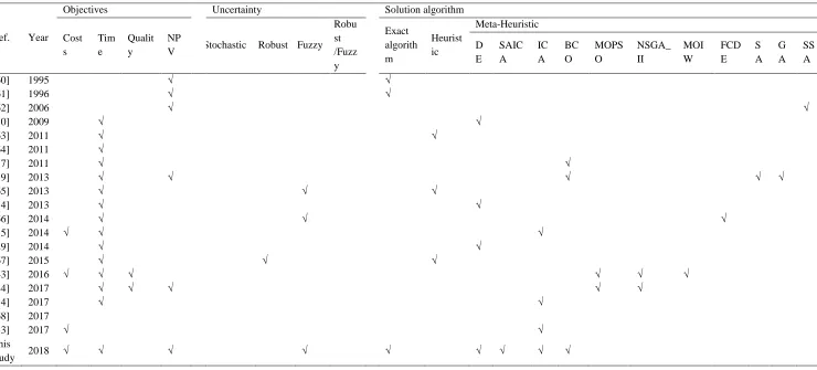
Aforementioned discussions and Table 1 show several gaps in the literature of RCPSP. The present study develops a new multi-objective mathematical programming under uncertainty for minimizing the completion time of the project, maximizing NPV of the project, and minimizing the costs of allocating workforces to perform the required skills of all activities. The main contributions of the present study which distinguishes it from the previous studies in this area are mentioned as below:

Developing a new multi-objective model of multi-mode RCPSP with interruption under an uncertain environment.

Utilizing a new two-phase framework consists of Me measure and TA method to cope with the uncertainty and the proposed multi-objective model, respectively.

Using a new meta-heuristic methods called SAICA and comparing the performance whit DE, ICO, and BCO method in order to successfully solve the large-sized problems in an acceptable time.

The remainder of the paper is expressed as follows: Section 2 gives an overview of the related literature. Section 3 proposes the problem description and a new mathematical model of RCPSP. Self-Adaptive Imperialist Competitive Algorithm (SAICA), Imperialist Competitive Algorithm (ICA), Bee Colony Optimization (BCO), and Differential Evolution (DE) are proposed as solution methods in Section 4. The next section is devoted to demonstrate the performance of the proposed methodology by solving the numerical example and two real case studies. Finally, analysis results of comparing the proposed SAICA with ICA, DE, BCO, and some offers for the future researches are given in the last section.

Aforementioned discussions and Table 1 illustrate several gaps in the literature of RCPSP. According to the best of our knowledge, only a few researchers have focused on maximizing NPV of the project. In addition, when the specific cash flows are paid during the project as cost to complete the project components, NPV is a substantial significant criterion in project scheduling [40]. On the other hand, considering the interruption of per activity because of some factors such as equipment failure and lack of resources make the project scheduling problem more realistic. Therefore, this paper proposes a new mathematical modeling to achieve the maximum NPV of the project so that each activity can be interrupted at any time and start again without adding any cost. Also, the present study works on another gap in the available literature by taking into consideration the new meta-heuristic method to solve the problem in an even more practical way.

Table 1. Review of related studies.

Ref. Year

Objectives Uncertainty Solution algorithm

Cost s Tim e Qualit y NP

V Stochastic Robust Fuzzy Robu st /Fuzz y Exact algorith m Heurist ic Meta-Heuristic D E SAIC A IC A BC O MOPS O NSGA_ II MOI W FCD E S A G A SS A

[60] 1995 √ √

[61] 1996 √ √

[62] 2006 √ √

[30] 2009 √ √

[63] 2011 √ √

[64] 2011 √

[37] 2011 √ √

[39] 2013 √ √ √ √ √

[65] 2013 √ √ √

[54] 2013 √ √

[66] 2014 √ √ √

[35] 2014 √ √ √

[29] 2014 √ √

[67] 2015 √ √ √

[43] 2016 √ √ √ √ √ √

[44] 2017 √ √ √ √ √

[34] 2017 √ √

[68] 2017

[33] 2017 √ √

This

2. Mathematical Formulation of RCPSP

RCPSP is a problem involves the set of n activities (j= {1, 2, …, n}) that two dummy activities 1 and n represent start and end of the project, respectively. It is noticeable to say that each activity should be processed in a specific duration time(𝑑_𝑗) without interruption and it needs some units (𝑟𝑗𝑘) of available resources (𝑅𝑗) during each period of its duration. There are two major

constraints in RCPSP. Firstly, each activity only can start after its predecessors activities (𝑃_𝑗). Secondly, each activity can be processed when the resources are available and the required resources cannot exceed the available resources 𝑅_𝑗. The objective is minimizing the completion time of the activities(𝐶𝑗) to obtain the best scheduling of activities due to their precedence and

the required resource units 𝑟_𝑗𝑘 of available resource 𝑅_𝑗 in specific time period 𝑡. Therefore, the above mentioned RCPSP formulation can be describe as follows:

min 𝐶𝑛 (1)

s.t

𝐶𝑗𝑃_𝑗  𝑑𝑗−𝑑𝑖 j=1 ,2, …, n (2)

∑ 𝑟𝑗𝑘

𝑗𝑆(𝑡): 𝐶𝑗−𝑑𝑗t 𝐶𝑛

 𝑅𝑗 k=1 ,2, …, n , 𝑡 ≥ 0 ₍₃₎

𝐶𝑛 ≥ 0 j=1 ,2, …, n (4)

Objective function (1) minimizes the completion time of activities. The precedence constraints between activates are guaranteed by Constraints (2). Constraint (3) implies the constraint of resource limitation where 𝑆(𝑡) shows a set of activates that they should be proceed at time t. Finally, the constraint of decision variables is shown by constraint (4).

In this section, a new mathematical model is proposed that minimizes the completion time of the project, maximizes the net present worth of the project, and minimizes the allocating workforces’ costs to perform required skills of all activities in RCPSP. The following assumptions are considered to formulate the model:

Activities are respectively numbered with 0 and N as dummy start and end activities.

The required resources to perform projects are renewable.

One or more sources are assigned to each activity.

Each activity can be interrupted at any time and start again without adding any cost.

Activities should be done in their earliest and latest time limitation.

Activities are allowed to start their activity in one mode and finish it in the same mode.

The amount of all multi-skill resources to perform each activity is predefined and available.

Each workforce is allowed to be assigned to only one skill of an activity at the same time.

The indices, parameters, and decision variables used in the mathematical model are shown below:

Sets

𝑖 Index of activities, 𝑖 = {0, … , 𝑛}

m Index of execution modes, 𝑚 = {1, … , 𝑀}

l Index of renewal resources,

w Index of workforce, 𝑤 = {1, … , 𝑊}

𝑡 Index of time to start activities, 𝑡 = {1, … , 𝑇𝑚𝑎𝑥}

h Index of skill, ℎ = {1, … , 𝐻}

Ai Set of activities, 𝑖 = {0, … , 𝑛}

A0 Virtual node of start activity, 𝑖 = 0

An Virtual node of finish activity, 𝑖 = 𝑛

(Ai, Aj) Set of perquisite relations between Ai, Aj

G(A, F, d) Perquisite graph

Parameters

P

̃_im Duration of activity i in mode m

T̃max Maximum amount of activities time, T̃max = ∑i𝑛𝑀𝑎𝑥(Pim1,…, PimM)

riml Amount of resource type 𝑙 for activity 𝑖 in mode m

Rl Amount of resource 𝑙 in each period

α Discount rate

Cf̃i Cash flow of each activity 𝑖

C̃wh Cost of performing skill ℎ by workforce w per unit time

qwh Quality of executing skill ℎ by workforce w

bimh Required number of workforces to perform skill ℎ of activity 𝑖 in mode 𝑚

rwh=1 If workforce 𝑤 has skill h; 0 otherwise

Decision variables

Cmax Completion time of project

NPVTit Temporary net present value of activity 𝑖 in time 𝑡

NPVi Net present value of activity 𝑖

Si Start time of activity 𝑖

Ci Completion time of activity 𝑖

gimt 1; if activity 𝑖 is started in mode 𝑚 at time 𝑡; 0 otherwise

𝑣im 1; if activity 𝑖 is done in mode 𝑚; 0 otherwise

ximwt 1; if activity 𝑖 is started in mode 𝑚 by workforce w at time 𝑡; 0otherwise

yimwh 1; if activity 𝑖 is performed in mode m by workforce w for skill ℎ 1; otherwise 0

Min 𝑍1=𝐶𝑚𝑎𝑥 (5)

Max 𝑍2=NPV (6)

Min 𝑍3= ∑ ∑ 𝑚𝑀

∑ ∑ (𝑦𝑖𝑚𝑤ℎ. C̃wh. P̃im) w𝑊

ℎ𝐻 𝑖𝐼

(7)

s.t

𝑁𝑃𝑉𝑇𝑖𝑡 = ∑ Cf̃i m𝑀

. 𝑒−𝛼𝑡. 𝑔𝑖𝑚𝑡 ∀ 𝑖, 𝑡 (8)

𝑁𝑃𝑉𝑖 = 𝑁𝑃𝑉𝑇𝑖𝑡 ∀ 𝑖, 𝑡 = T̃max (9)

𝑁𝑃𝑉𝑖≥𝑁𝑃𝑉𝑇𝑖𝑡 ∀ 𝑖, 𝑡 (10)

𝑥𝑖𝑚𝑤𝑡≤𝑣𝑖𝑚 ∀ 𝑖, 𝑚, 𝑤, 𝑡 (11)

𝑦𝑖𝑚𝑤ℎ≤𝑣𝑖𝑚 ∀ 𝑖, 𝑚, 𝑤, 𝑡 (12)

∑ 𝑚𝑀

∑ 𝑥𝑖𝑚𝑤𝑡 t𝑇

≤ 1 ∀ 𝑖, 𝑤 ₍₁₃₎

𝑦𝑖𝑚𝑤ℎ≤𝑟𝑤ℎ ∀ 𝑖, 𝑚, 𝑤, 𝑡,

ℎ (14)

𝑥𝑖𝑚𝑤𝑡≤𝑔𝑖𝑚𝑡 ∀ 𝑖, 𝑚, 𝑤, 𝑡 (15)

𝑥𝑖𝑚𝑤𝑡+ 1 ≥ 𝑔𝑖𝑚𝑡+ ∑ 𝑦𝑖𝑚𝑤ℎ h𝐻

∀ 𝑖, 𝑚, 𝑤, 𝑡

∑ 𝑤𝑊

∑ 𝑥𝑖𝑚𝑤𝑡 t𝑇

= ( ∑ 𝑏𝑖𝑚ℎ h𝐻

) . 𝑣𝑖𝑚

∀ 𝑖, 𝑚

(17)

∑ 𝑦𝑖𝑚𝑤ℎ w𝑊

= 𝑏𝑖𝑚ℎ. 𝑣𝑖𝑚 ∀ 𝑖, 𝑚, ℎ ₍₁₈₎

∑ 𝑚𝑀

∑ 𝑖𝑛

∑ 𝑥𝑖𝑚𝑤𝑑

𝑠=𝑡−𝑃𝑖𝑚+1𝑇

≤ 1 ∀ 𝑤, 𝑡 ₍₁₉₎

∑ 𝑡𝑇

∑ 𝑥𝑖𝑚𝑤𝑡 m𝑀

= ∑ ℎ𝐻

∑ 𝑦𝑖𝑚𝑤ℎ m𝑀

∀ 𝑖, 𝑤

(20)

∑ 𝑣𝑖𝑚 m𝑀

= 1 ∀ 𝑖 ₍₂₁₎

∑ 𝑔𝑖𝑚𝑡= t𝑇

𝑣𝑖𝑚. P̃im ∀ 𝑖, 𝑚 ₍₂₂₎

𝑆𝑖≤ t. 𝑔𝑖𝑚𝑡 + (1-𝑔𝑖𝑚𝑡) . M ∀ 𝑖, 𝑚, 𝑡 (23)

𝐶𝑖≥ t. 𝑔𝑖𝑚𝑡 ∀ 𝑖, 𝑚, 𝑡 (24)

𝐶𝑚𝑎𝑥≥𝐶𝑖 ∀ 𝑖 (25)

𝐶𝑖≤𝑆𝑗 ∀ 𝑖, 𝑗 (26)

∑ 𝑖𝑛

∑ 𝑟𝑖𝑚𝑙. 𝑔𝑖𝑚𝑡 m𝑀

≤ 𝑅𝑙 ∀ 𝑖, 𝑡 (27)

𝑥𝑖𝑚𝑤𝑡 , 𝑦𝑖𝑚𝑤ℎ , 𝑔𝑖𝑚𝑡 , 𝑣𝑖𝑚 ∈ {0,1} ∀ 𝑖, 𝑚, 𝑤, ℎ, t (28)

The proposed model includes three objective functions. Objective function (5) aims to minimize the completion time of the project. Objective (6) maximizes NPV of the project. Objective (7) minimizes the related costs of allocating workforces to fulfill the required skills of all activities. NPV is determined by Constraint (8) and Constraint (9) guarantees that the maximum NPV of each activity is limited. Constraint (10) embodies that NPV of each activity is more than its temporary NPV at any time. The logical relations between 𝑥_{𝑖𝑚𝑤𝑡} and 𝑣_𝑖𝑚, and the reasonable relations between 𝑦𝑖𝑚𝑤ℎ and 𝑣𝑖𝑚 are guaranteed by Constraints (11) and Constraint (12),

equal to the required workforce numbers with skill h to execute that activity. Constraint (19) illustrates that the allocated resources of each mode will be fixed from start to the end of an activity. Constraint (20) guarantees that a workforce should start his work during the project time horizon, if he/she be assigned to skill k of activity 𝑖. Constraint (21) forces each activity to carry out and finish in the same mode. Constraint (22) makes balance between the total time of doing activity 𝑖 in mode 𝑚_𝑖 at time t and time of getting performed in mode 𝑚_𝑖. The start time of activity is shown by Constraint (23). Constraint (24) determines the completion time of activities. The minimum limitation of competition time is illustrated in Constraint (25). Constraint (26) identifies the perquisite relations between activities. Constraint (27) attempt to limit the renewal resources access level that is not allowed to be more than a determined amount. Constraint (28) is the logical binary necessity on the decision variables.

2.1 Validating the Proposed Model

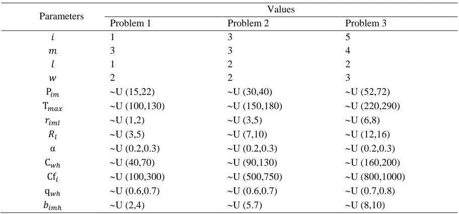
In this section, the problem number 1 in Table 2 is considered as a small-sized test problem (i.e. 𝑖  𝑚  l  w = 1  3  1  2 ). Also, three problems are solved and coded in GAMS 22.9 software and solved by CPLEX solver due to the data sets generated randomly, and listed in Table 2. In addition, the results summary of obtained objective functions values of TH method are illustrated in Table 3.

Table 2. Data sets generated randomly.

Parameters Values

Problem 1 Problem 2 Problem 3

𝑖 1 3 5

𝑚 3 3 4

𝑙 1 2 2

𝑤 2 2 3

P𝑖𝑚 U (15,22) U (30,40) U (52,72)

T𝑚𝑎𝑥 U (100,130) U (150,180) U (220,290)

𝑟𝑖𝑚𝑙 U (1,2) U (3,5) U (6,8)

𝑅𝑙 U (3,5) U (7,10) U (12,16)

α U (0.2,0.3) U (0.2,0.3) U (0.2,0.3)

C𝑤ℎ U (40,70) U (90,130) U (160,200)

Cf𝑖 U (100,300) U (500,750) U (800,1000)

q𝑤ℎ U (0.6,0.7) U (0.6,0.7) U (0.7,0.8)

Table 3. Summary results of test problems by TH method for  = (0.5,0.2,0.3) and 𝝑 =0.6. Problem

No.

OFV1 μ1(Z) OFV2 μ2(Z) OFV3 μ3(Z)

1 2301.03 0.962 12910.82 0.865 27735.01 0.952

2 5310.91 0.901 28765.32 0.941 42930.19 0.964

3 15275.55 0.930 62820.19 0.791 74319.58 0.881

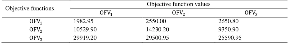
The proposed multi-objective model is solved separately as three single-objective problems in order to verify the validity of the presented model. Different results obtained due to each objective function are shown in Table 4 and the results show that there is a conflict between three objective functions. It is worthwhile to say that the obtained results are related to the problem number 1 as a small-sized problem. Table 4 shows that when the optimal solutions obtain regarding one objective function without considering the factors considered in other objective functions, the other objective functions will get the worst values. As one, when the optimal solutions obtain due to the first objective function without considering the factors considered in other objective functions, the first objective function (minimizing the total duration time) decreases to 1982.95. This is while the second objective value, which is maximizing the NPV of the project, is decreased to 10529.90 and the second objective value which attempts to achieve the minimized amount of the total costs is increased to 29919.20.

Table 4. Summary results of solving every objective function separately for problem number 1.

Objective functions Objective function values

OFV1 OFV2 OFV3

OFV1 1982.95 2550.00 2650.80

OFV2 10529.90 14230.20 9350.90

OFV3 29919.20 29500.95 25590.95

3. Solution Method

Imperialist Competitive Algorithm (ICA), and Self-adaptive Imperialist Competitive Algorithm (SAICA).

3.1 Equivalent Auxiliary Crisp Model

In the literature, there are various methods to transform a possibilistic model into the equivalent auxiliary crisp one such as the expected value operator and the chance constrained programming approach. Also, several methods attempt to transform possibilistic model into the equivalent auxiliary crisp one by using the chance constrained programming approach. In the literature, the optimistic and pessimistic attitudes of Decision Makers (DMs) are introduced by the possibility measures (Pos) and the necessity measure (Nec) as the basic fuzzy measures [42]. It is because the optimistic attitude and pessimistic attitude, respectively leads to lose the constraints and make the constraints tight. Xu et al. [42] proposed a more flexible measure namely Me to avoid extreme attitudes. Besides, Me measure is able to consider the combined attitude of DM, which is something between optimistic and pessimistic views. In the following, a possibility space introduced by Dubois et al. [43] shown as the triple (, P(), Pos) where , P(), and Pos are a non-empty set, respectively, the power set of , and a possibility measure. Xu et al. [42] introduced the fuzzy measure Me as follows:

M{𝐴} Nec{𝐴}   (Pos{𝐴} Nec{𝐴}), (29)

where A is a set in P() and λ is the optimistic-pessimistic parameter to determine the combined attitude of the DM. Also, Pos{𝐴} and Nec{𝐴} show the possibility and necessity of set A in the possibility space, respectively. Based on Xu et al. [42], the expected value operator based on the Me measure can be define as follows:

E[](1)

2 1 1 2 2



2 3, (30)

where (₁, ₂, ₃) is a triangular fuzzy variable. In the Me-based possibilistic programming method, the expected value and the chance-constrained operators are applied to cope with the possibilistic model as follows:

Min 𝑐̃ 𝑥

(31) s.t

Me{𝐴̃𝑥  𝑏̃}  α

Me{𝑁̃𝑥  𝑑̃}  

𝑥 ≥ 0.

Where 𝑐̃  (𝑐̃₁, 𝑐̃₂, … , 𝑐̃_𝑛), 𝐴̃ [𝑎̃_𝑖𝑗]_𝑚𝑛, 𝑁̃  [𝑛̃_𝑖𝑗]_𝑚𝑛, 𝑏̃  (𝑏̃₁, 𝑏̃₂, … , 𝑏̃_𝑛)𝑡_{, and 𝑑̃ }

Also, α and  are the DM’s minimum confidence level of possibilistic constraints that should be satisfied.

Based on Xu et al. [42], the above model can be transformed into two approximation models, namely the Lower Approximation Model (LAM) and the Upper Approximation Model (UAM) that are illustrated as follows:

(𝑈𝐴𝑀) =

{

Min E[𝑐̃]x 𝑠. 𝑡. Pos{𝐴̃𝑥  𝑏̃}  𝛼 Pos{𝑁̃𝑥  𝑑̃} 

𝑥 ≥ 0

(32)

and

(𝐿𝐴𝑀) =

{

Min E[𝑐̃]x 𝑠. 𝑡. Nec{𝐴̃𝑥  𝑏̃}  𝛼 Nec{𝑁̃𝑥  𝑑̃} 

𝑥 ≥ 0

(33)

The above possibilistic models can be transformed into two crisp equivalent models as Eq. (34) and Eq. (35).

(𝑈𝐴𝑀) =

{

Min (1 − 2 𝐶(1)

1 2𝐶(2)

 2𝐶(3)) x 𝑠. 𝑡.

𝐴(2)𝑥  (1 𝛼)(𝐴(3)𝐴(2))x  𝑏(2) (1 𝛼)(𝑏(2)𝑏(1)) 𝑁(2)𝑥  (1)(𝑁(2)𝑁(1))x  𝑑(2) (1)(𝑑(3)𝑑(2))

𝑥 ≥ 0

(34)

and

(𝐿𝐴𝑀) =

{

Min (1 − 2 𝐶(1)

1 2𝐶(2)

 2𝐶(3)) x 𝑠. 𝑡.

𝐴(2)𝑥  α(𝐴(2)𝐴(1))x  𝑏(2) (1 𝛼)(𝑏(3)𝑏(2)) 𝑁(2)𝑥  (1)(𝑁(3)𝑁(2))x  𝑑(2)(𝑑(2)𝑑(1))

𝑥 ≥ 0

(35)

UAM:

Min 𝑍1=𝐶𝑚𝑎𝑥 (36)

Max 𝑍2=NPV (37)

Min 𝑍3

= ∑ ∑ 𝑚𝑀

∑ ∑ (𝑦𝑖𝑚𝑤ℎ. ( 1 −

2 𝐶𝑤ℎ(1) 1

2𝐶𝑤ℎ(2) 

2𝐶𝑤ℎ(3)). ( 1 −

2 𝑃𝑖𝑚(1) 1

2𝑃𝑖𝑚(2) 

2𝑃𝑖𝑚(3))) w𝑊

ℎ𝐻 𝑖𝐼

(38)

s.t

𝑁𝑃𝑉𝑇𝑖𝑡 = ∑ (𝐶𝑓𝑖(2)+ (1 − 𝛼)(𝐶𝑓𝑖(3)− 𝐶𝑓𝑖(2)) m𝑀

. 𝑒−𝛼𝑡. 𝑔𝑖𝑚𝑡 ∀ 𝑖, 𝑡 (39)

∑ 𝑔𝑖𝑚𝑡 = t𝑇

𝑣𝑖𝑚. (𝑃𝑖𝑚(2)+ (1 − 𝛼)(𝑃𝑖𝑚(3)− 𝑃𝑖𝑚(2)) ∀ 𝑖, 𝑚 (40)

Other constraints

LAM:

Min 𝑍1 =𝐶𝑚𝑎𝑥 (41)

Max 𝑍2 =NPV (42)

Min E[𝑍3] (43)

s.t

𝑁𝑃𝑉𝑇𝑖𝑡 = ∑ (𝐶𝑓𝑖(2)− (𝛼)(𝐶𝑓𝑖(2)− 𝐶𝑓𝑖(1)) m𝑀

. 𝑒−𝛼𝑡_{. 𝑔}

𝑖𝑚𝑡 ∀ 𝑖, 𝑡 ₍₄₄₎

∑ 𝑔𝑖𝑚𝑡= t𝑇

𝑣𝑖𝑚. (𝑃𝑖𝑚(2)− (𝛼)(𝑃𝑖𝑚(2)− 𝑃𝑖𝑚(1)) ∀ 𝑖, 𝑚 ₍₄₅₎

Other constraints.

3.2 Fuzzy Interactive Method

Step 1. Define the related Positive Ideal Solution (PIS) and Negative Ideal Solution (NIS) of each objective function.

Step 2. Identify a linear membership function for each objective function as Eq. (46) and Eq. (47) to minimize and maximize the objective function, respectively.

Μk(𝒵) =

{

1 if 𝒵k < 𝒵kPIS 𝒵kNIS− 𝒵k

𝒵_kNIS− 𝒵_kPIS if 𝒵k PIS_{≤ 𝒵}

k≤ 𝒵kNIS

0 if 𝒵k > 𝒵kNIS

(46)

μk(𝒵) =

{

1 if 𝒵k< 𝒵kPIS 𝒵k− 𝒵kNIS

𝒵_kPIS− 𝒵_kNIS if 𝒵k PIS_{≤ 𝒵}

k≤ 𝒵kNIS

0 if 𝒵k > 𝒵kNIS

(47)

Step 3. Convert the proposed multi-objective model into a single-objective one by applying the TH aggregation function. The TH aggregation function is determined by the following equations:

max ψ(𝑋) = 𝜗𝜆0+ (1 − 𝜗) ∑ 𝜑𝑘𝜇𝑘(𝒵)

𝑘 (48)

s.t

𝜆0 ≤ 𝜇𝑘(𝒵) 𝑘 = 1, 2, 3 (49)

𝑥 ∈ 𝐹(𝑥) 𝜆0, 𝜓 ∈ [0,1] (50)

Where 𝐹(𝑥), 𝜗, and 𝜑_𝑘 (∑ 𝜑_{𝑘 𝑘} = 1) indicate the feasible region, the coefficient of compensation, and the relative importance of the k𝑡ℎ objective function, respectively. In addition, 𝜇_𝑘(𝒵) and 𝜆₀ = min {𝜇_𝑘(𝒵)} illustrate the satisfaction degree of the k𝑡ℎ objective function and the minimum satisfaction degree of objectives, respectively. Also, through this manner, the DMs are able to control the minimum of the objective functions and the compromise degree among them implicitly due to their preferences.

Step 4. Solve the single-objective model due to the given coefficient of compensation 𝜗 and the relative importance of the objective functions 𝜑_𝑘. If the decision maker is satisfied with the obtained efficient compromise solution, stop; otherwise, change the value of mentioned parameters to achieve another compromise solution.

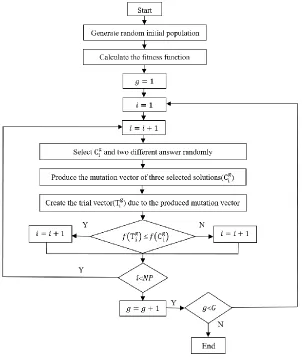
3.3 Differential Evolution (DE)

proposed by Storn et al. [46] for the first time, and it works based on the initial population to find the optimal solutions of optimization problems. The most typical feature of DE is that it has speed. On the other word, it uses an efficient search process in the direction of optimistic variables. Also, it can change wrong directions into correct directions. This feature means that DE has speed [47]. There are three main operations of DE: Mutation, Crossover, and Selection; they are repeated for predefined iterations. 𝐶_𝑖𝑔 denotes the initial solutions where 𝑔 and 𝑖 states the generation and the individuals, respectively. To generate the trial vectors, the Mutation and Crossover are utilized and after that the vectors can be done by selection to survive into the next generation. Every operation of DE is described below:

3.3.1 Mutation

Similar to Genetic Algorithm (GA), DE, utilizes C_ig and C₁g− C₂gas two parents of the population to create new child (M_ig). Also, rand_j,ig shows a vector of random elements in the range [0, 1] where j is the element index of the solution vector. Eq. (51) shows that how three different solutions are combined to produce a mutated vector and A is a pre-defined real-valued factor that controls evolution rate of the population:

M_j,ig= C_j,ig+ A randg_j,i(C_j,1g − C_j,2g ) (51)

3.3.2 Crossover

After creating mutation vector, M_ig, it will be combined by the solution, C_ig and after that the crossover operation is processed by DE. Therefore, the trial vector, T_j,ig, can be produced by following equation:

T_j,ig={Mj,i g

𝑖𝑓 (r_j,ig 𝐶𝑟 𝑜𝑟 𝑗 = 𝑗𝑟)

C_j,ig 𝑜𝑡ℎ𝑒𝑟𝑤𝑖𝑠𝑒 (52)

Where Cr[0,1] is a crossover factor to determine the elements of T_j,ig.

3.3.3 Selection

In selection operation, due to Eq. (52) the trial vector, T_j,ig, is compared based on the objective function amount, C_ig. The solution by the better fitness function would be move to the next generation as the new solution, C_ig+1, and the other solution should be eliminate:

T_j,ig={T i g

𝑖𝑓 𝑓(T _ig)  𝑓(C _ig)

To the better understanding of the DE function, the flowchart of DE is illustrated in Figure 5. Meanwhile, 𝑓(T _ig) and 𝑓(C _ig) represent the fitness function for the trial victor and the amount objective functions, respectively. In addition, 𝑔 and 𝑖 state the generation and the individuals, respectively.

3.4 Bee Colony Optimization (BCO)

The Bee Colony Optimization (BCO) meta-heuristic is inspired by bees' behavior in the nature. It means, it is a biologically inspired method that explores the collective intelligence applied by the honey bees during nectar collecting process to deal with combinatorial optimization problems. BCO is used by Luic and Teodorovic [48, 49, 50] for the first time to solve their problem based on the basic principles of collective bee intelligence. BCO is based on the basic idea of creating the multi agent system (colony of artificial bees) in order to solve the difficult combinatorial optimization problems. The artificial bee colony behaves partially differently from bee colonies in nature.

Figure 1. Flowchart of Deferential Evolution (DE).

Initialization: every bee is set to an empty solution; For every bee do the forward pass:

a. Set k = 1; counter for constructive moves in the forward pass; b. Evaluate all possible constructive moves;

c. According to evaluation, choose one move using the roulette wheel; d. k = k + 1; If k ≤ NC Go to step b.

All bees are back to the hive; // backward pass starts; Sort the bees by their objective function value;

Every bee decides randomly whether to continue its own exploration and become a recruiter, or to become a follower

(bees with higher objective function value have greater chance to continue its own exploration); For every follower, choose a new solution from recruiters by the roulette wheel;

If the stopping condition is not met, Go To step 2; Output the best result

3.5 Imperialist Competitive Algorithm (ICA)

An Imperialist Competitive Algorithm (ICA) is an evolutionary method proposed by Atashpaz-Gargari et al. [51] for the first time. ICA starts its work due to a basic solution which is the initial population is called country. The country consists of imperialists and colonies that the best countries in the population refer to the imperialists; the countries of the imperialists that are divided among the imperialists due to their power are the colonies [52]. Then, both imperialists and that is why their colonies create the initial empires. The colonies should be distributed among empires to start the competition between imperialists of the empires; calculating the total power of the empire includes the imperialists; colony power is a substantially significant issue. Therefore, the total power of an empire can be defined as the power of imperialist country summation plus the percentage of mean power of its colony. The objective of ICA is to find the optimal solution of the problems. This algorithm has been used in the literature several times [31, 53].

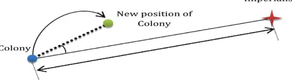
Thenceforth, colonies start to move toward their relevant imperialist through an assimilation. Figure 3 illustrates the assimilation operator in details. After that, the competition is beginning among the imperialists of the empires; those empires that are not able to increase their power are not successful and going to be removed. Therefore, the empires which are weak will miss their power slowly and ultimately they will collapse. At the end, all countries will converge to a situation by which just one empire exists and the other countries are the colonies of that empire because of the competition among the empires and the collapse mechanism. In Figure 3, a random deviation value is added to deviate the direction of movement. In addition, the random number with uniform distribution and the distance between colony are shown by 𝜃 and d, respectively.

Figure 3. Assimilation operator with a random angle. 3.6 Self-Adaptive Imperialist Competitive Algorithm (SAICA)

substantially significant feature of this algorithm is that the several crossover operators are utilized at the same time without increasing the time of computation.

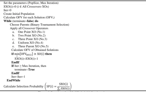
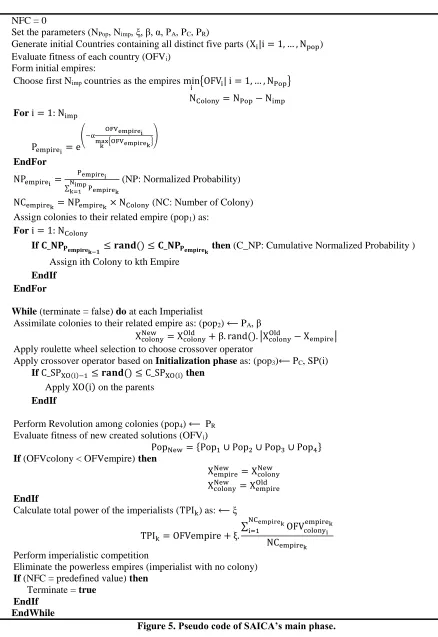
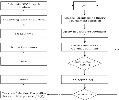
There are two phases in SAICA: Initialization and main phase. In initialization phase, each crossover operator obtains a score rather than other operators whenever it would be able to create more acceptable solution at every iteration. Then, the Selection Probability (SP) metric of each operator is calculated after the already defined number of iterations by dividing the obtained score by number of iteration; the focal factor is Σ 𝑆𝑃 = 1. At the end of the initialization phase, the main phase is started to search the solution space by utilizing the assimilation, self-adapted crossover, and revolution operators. This study used the crossover contains one point, two points, three points, uniform, and three parent crossover operators [54]. Figure 4 and Figure 5 illustrate the pseudo codes of the initialization and main phase of proposed SAICA, respectively. To easier understanding of the proposed approach, Figure 6 and Figure 7 are depicted too [55].

Set the parameters (PopSize, Max Iteration) SXO(i)=0 (i ∈ All Crossovers-XOs)

Iter=0

Create Initial Population

Calculate OFV for each Solution (OFVi)

While (terminate=false) do

Choose Parents (Binary Tournament Selection) Apply all Crossover Operators

a. One Point XO (No.1) b. Two Point XO (No.2) c. Three Point XO (No.3) d. Uniform XO (No.4) e. Three Parent XO (No.5) Calculate OFV of Obtained Solutions 𝐈𝐟 min

i {OFVXO(i)} ≅ XO(i) 𝐭𝐡𝐞𝐧

SXO(i)=SXO(i)+1 EndIf

If Iter ≥ Max Iteration, then terminate=True

EndIf Iter=Iter+1 EndWhile

Calculate Selection Probabilty (SP(i) = SXO(i) ∑ SXO(i)i

)

Figure 4. Pseudo code of SAICA’s initialization phase. 4. Computational Results

NFC = 0

Set the parameters (NPop, Nimp, ξ, β, α, PA, PC, PR)

Generate initial Countries containing all distinct five parts (Xi|i = 1, … , Npop)

Evaluate fitness of each country (OFVi)

Form initial empires:

Choose first Nimp countries as the empires min

i {OFVi| i = 1, … , NPop}

NColony= NPop− Nimp

Fori = 1: Nimp

Pempire_i = e

(−α OFVempirei

max

k {OFVempirek}

)

EndFor

NPempire_i =

P_empirei

∑Nimp_k=1 P_empirek

(NP: Normalized Probability) NCempire_k = NPempire_k× NColony (NC: Number of Colony)

Assign colonies to their related empire (pop1) as:

For i = 1: NColony

If 𝐂_𝐍𝐏𝐏_{𝐞𝐦𝐩𝐢𝐫𝐞𝐤−𝟏} ≤ 𝐫𝐚𝐧𝐝() ≤ 𝐂_𝐍𝐏𝐏_{𝐞𝐦𝐩𝐢𝐫𝐞𝐤} then (C_NP: Cumulative Normalized Probability )

Assign ith Colony to kth Empire EndIf

EndFor

While (terminate = false) do at each Imperialist

Assimilate colonies to their related empire as: (pop2) ⟵ PA, β

XcolonyNew = XcolonyOld + β. rand(). |XcolonyOld − Xempire|

Apply roulette wheel selection to choose crossover operator

Apply crossover operator based on Initialization phase as: (pop3)⟵ PC, SP(i)

If C_SPXO(i)−1≤ 𝐫𝐚𝐧𝐝() ≤ C_SPXO(i) then

Apply XO(i) on the parents EndIf

Perform Revolution among colonies (pop4) ⟵ PR

Evaluate fitness of new created solutions (OFVi)

PopNew= {Pop1∪ Pop2∪ Pop3∪ Pop4}

If (OFVcolony < OFVempire) then

XempireNew = XcolonyNew

XcolonyNew = XempireOld

EndIf

Calculate total power of the imperialists (TPIk) as: ⟵ ξ

TPIk = OFVempire + ξ.

∑ OFV_colony

i

empire_k NC_empirek

i=1

NCempire_k

Perform imperialistic competition

Eliminate the powerless empires (imperialist with no colony) If (NFC = predefined value) then

Terminate = true EndIf

EndWhile

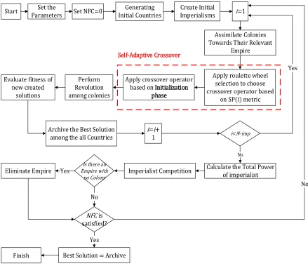
Figure 6. Flowchart of the initialization phase. 4.1 Sensitive Analysis

In his section, some several small-size test problems are analyzed based on the data of Table 2 to investigate the correctness of the presented model. Table 5 illustrates the several sensitivity that is done on the small-size test problem under different values of 𝜗 and 𝜑 to check the effects of these parameters values alterations on the objective functions. The obtained results by Table 5 show that changing the values of 𝜑 has a significant influence on each OFV, so that the better objective function value is obtained when the value of 𝜑 is hanged by DM according to the objective functions preferences to gain the better value of them. Similarly, changing the 𝜗-value will change the objective function values and their satisfaction degrees; DM is able to set the value of 𝜗 to achieve the best value of the satisfaction degrees. For example, according to Table 5, changing the values of 𝜑 increases the satisfaction degree associated with first, second, and third objective functions from 0.791 to 0.62, 0.865 to 0.952, and 0.865 to 0,966.

Calculate OFV for each

Solution j=1

Choose Parents using Binary Tournament Selection

i <Max Iter

Yes

Calculate Selection Probability

for each XO Operator (SP(i)) No

Apply all Crossover Operators - XOi

Calculate OFV for New Obtained Solutions

mini (OFVXO(i))

≊XO(i)

SXO(i)=SXO(i)+1 Finish

Generating Initial Population

Set SXO(i)=0

Set the Parameters

Figure 7. Flowchart of the main phase.

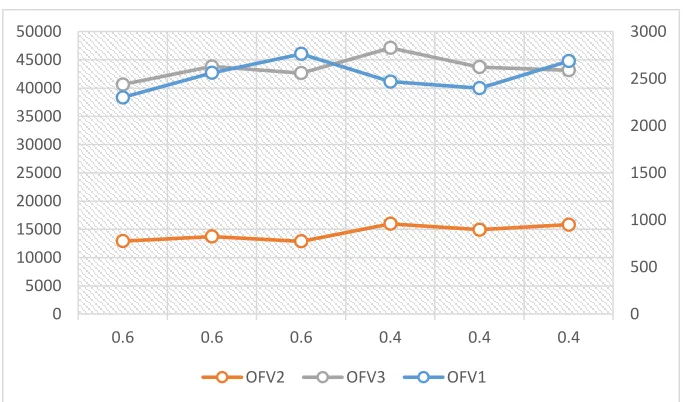
Also, Figure 8 to Figure 10 illustrate the value of each objective function obtained by TH method for three small-size test problems. In addition, Figure 11 shows the changes in OFV3 versus cost of performing each skill. It is obvious that increasing the value of performing each skill cost leads to achieve the worse value of this objective function. On the other word, it is because increasing the value of performing each skill cost enforces more costs to the system; it will increase OFV3, as well.

Start Set the Parameters

Generating Initial Countries

Create Initial

Imperialisms i=1

Assimilate Colonies Towards Their Relevant

Empire

NFC is satisfied?

Finish

Apply roulette wheel selection to choose crossover operator based

on SP(i) metric

i=i+

1 i<N-imp

Yes

Calculate the Total Power of imperialist

No

Imperialist Competition Is there an

Empire with no Colony Eliminate Empire Yes

No

No

Best Solution = Archive Yes

Set NFC=0

Apply crossover operator based on Initialization

phase Perform

Revolution among colonies Evaluate fitness of

new created solutions

Archive the Best Solution among the all Countries

Table 5. Summary results of test problems.

Problem No. 𝜗 𝜑 𝑂𝐹𝑉1 𝜇1(𝑍) 𝑂𝐹𝑉2 𝜇2(𝑍) 𝑂𝐹𝑉3 𝜇3(𝑍)

1

0.6 (0.5,0.2,0.3) 2301.03 0.962 12910.82 0.865 27735.01 0.952 0.6 (0.3,0.3,0.3) 2561.23 0.901 13722.95 0.887 30091.76 0.889 0.6 (0.2,0.4,0.4) 2763.45 0.791 12863.41 0.851 29782.71 0.901 0.4 (0.5,0.2,0.3) 2468.83 0.932 15982.01 0.952 31129.21 0.865 0.4 (0.3,0.3,0.3) 2398.10 0.951 14929.41 0.918 28797.01 0.923 0.4 (0.2,0.4,0.4) 2686.92 0.882 15823.01 0.941 27345.49 0.966

2

0.6 (0.5,0.2,0.3) 5310.91 0.901 28765.32 0.941 42930.19 0.964 0.6 (0.3,0.3,0.3) 5420.98 0.881 27863.54 0.910 44938.20 0.910 0.6 (0.2,0.4,0.4) 5298.18 0.919 26159.40 0.881 46382.02 0.859 0.4 (0.5,0.2,0.3) 5109.29 0.923 25901.84 0.841 50354.01 0.771 0.4 (0.3,0.3,0.3) 5542.30 0.859 27936.72 0.922 410387.2 0.998 0.4 (0.2,0.4,0.4) 5296.88 0.910 30971.59 0.981 45397.21 0.890

3

0.6 (0.5,0.2,0.3) 15275.55 0.930 62820.19 0.791 74319.58 0.881 0.6 (0.3,0.3,0.3) 16861.09 0.902 67384.12 0.932 75018.21 0.863 0.6 (0.2,0.4,0.4) 15570.19 0.923 65493.20 0.882 76367.10 0.821 0.4 (0.5,0.2,0.3) 17631.98 0.801 65938.10 0.891 73298.45 0.910 0.4 (0.3,0.3,0.3) 16981.99 0.881 68346.14 0.953 72093.11 0.974 0.4 (0.2,0.4,0.4) 17230.64 0.862 69201.52 0.964 72938.13 0.954

Figure 8. Objective function values of the TH method for test problem 1.

0 500 1000 1500 2000 2500 3000

0 5000 10000 15000 20000 25000 30000 35000 40000 45000 50000

0.6 0.6 0.6 0.4 0.4 0.4

Figure 9. Objective function values of the TH method for test problem 2.

Figure 10. Objective function values of the TH method for test problem 3.

4800 4900 5000 5100 5200 5300 5400 5500 5600

0 50000 100000 150000 200000 250000 300000 350000 400000 450000 500000

0.6 0.6 0.6 0.4 0.4 0.4

OFV2 OFV3 OFV1

14000 14500 15000 15500 16000 16500 17000 17500 18000

0 20000 40000 60000 80000 100000 120000 140000 160000

0.6 0.6 0.6 0.4 0.4 0.4

Figure 11. OFV3 vs. cost of performing each skill. 4.2 Performance Evaluation

This section investigates the efficiency of the proposed SAICA, the quality of solutions, and the computation time through a comparison study. At first, a typical example and two real case studies of RCPSP in literature review are investigated. Finally, a real case study of RCPSP is investigated to shows the efficiency of the proposed method.

4.2.1 Test problem 1

In this section, the solution quality and the computational time of the proposed SAICA is investigated through a comparative study. Therefore, a typical RCPSP example from Wu et al. [56] were used and it is shown by Figure 12 to illustrate the precedence relationships among the activities by arrow line. In addition, in mentioned example, 25 activities and two dummy activities with three types of renewable resource are considered. Some activities (i.e. activity 20 and 35) needs two types of resources whereas others require three types. Also, only one mode is considered in this problem. The required amount of resources and also, the time duration of each project activity is indicated above and below the corresponding circle node, respectively. Choosing the appropriate initial control parameters of meta-heuristic algorithms are really important, because it leads to both flexible and efficient solutions and surely it effects on the proposed model performances [57]. So, the most effective parameters which are required for investigating SAICA are shown in Table 6.

0 500 1000 1500 2000 2500 3000 3500

Figure 12. A typical RCPSP example [57].

Table 6. Parameters setting for SAICA.

Parameters Values

Population size 100

Imperialist No 8

Assimilation Rate 0.8

Revolution Rate 0.2

 0.05

 1.6

NFC 5000

The mentioned RCPSP example is solved in Matlab 2014 software environment and then the proposed SAICA results are compared with the results of the DE as a meta-heuristic algorithm. Table 7 embodies the results obtained by the proposed approach consist of both obtained minimum project duration and the computational times of achieving the best scheduling scheme and also, the calculated average deviation from computation time of the illustrated example by utilizing the above algorithms.

Table 7. The statistic results of project duration and CPU time in 30 runs. Scheduling

approach

Project duration Computation time

Min Average Max Std

DE 68 3.14 9.70 12.32 0.84

BCO 67 2.98 8.89 11.60 0.98

ICA 66 0.31 4.70 8.70 0.87

SAICA 64 0.51 5.16 9.82 0.96

4.2.2 Test problem 2

Based on two real case studies of literature review investigated by Jun et al. [57] and Chen et al. [58], the present study utilizes SAICA, ICA, BCO, and DE approaches to find the corresponding optimal solution schedules. The 20 activities with varying daily resource demands and 37 activities by one renewable resource are considered in case study 1 and 2, respectively, and are shown by Figure 13 and Figure 14. In addition, it is worth noting that there is a limitation of 9 resources every day for case study 1 and a maximum limit of 12 labors every day for case study 2. Also, only one mode is considered in this problem. It is worthwhile to say that in Figure 13 the required time duration of each project activity is indicated above the corresponding circle node and similarly in Figure 14. The time duration of each project activity and also the required labor for each activity is indicated above and below the corresponding circle node, respectively. The summery results of running the problem for 30 times are shown in Table 4 and it confirms the usefulness of the solution method.

Figure 13. A typical RCPSP example with a daily resource limit=9 [58].

Table 8. The summary of results for two case studies after 30 runs. No.

problem

Approach Success rate

Optimal value Computation time

Min Average Std Max Min Average Std Max

1 DE 73.33% 42.0 42.50 0.86 44.00 2.34 5.57 3.78 12.91 BCO 79.55% 42.0 42.41 0.86 43.79 2.29 5.17 2.60 1.07

ICA 89.34% 42.0 42.38 0.85 43.31 1.95 4.70 2.28 9.81 SAICA 96.00% 42.0 42.10 0.84 42.90 2.17 5.23 2.54 10.9 2 DE 70.00% 190 191.27 2.02 196.02 8.87 62.21 4.86 102.6

BCO 78.81% 190 190.92 1.49 195.13 6.33 56.71 4.50 96.12 ICA 90.03% 190 190.57 1.07 193.41 5.76 51.57 4.09 87.39 SAICA 95.00% 190 190.07 0.85 191.73 6.40 57.30 4.55 97.10

4.2.3 Case study

In this section, a car parts manufacturer company, namely P.C is selected as a real case of RCPSP to verify our mathematical model and the proposed methods performance. The automotive industry is one of the largest industries in Iran, and because of that the project scheduling of manufacturing the required car parts has triggered a substantially significant issue among researchers, recently. In addition, this is a real case study in which the interruption can be occur for per activity of some factors such as equipment failure and lack of resources. Therefore, the proposed model of the present study attempts to minimize the completion time of the project, maximize the NPV of the project, and minimize the allocating workforces’ costs to perform required skills of all activities.

In this study, the statistical data related to the problem are obtained from different sources to run the proposed model. We have considered 51 activities of P.C manufacturing company and the required data is shown by Table 9. In addition, the duration of each activity (𝑝_𝑖𝑚), Maximum amount of activities time (𝑇𝑚𝑎𝑥), resource amount if each type for every activity in each mode

Table 9. Data sets of the real case study.

In this study, two scenarios are considered: 1) considering precedence relationships only, 2) considering precedence relationships and resource constraints. According to Figure 15, when only the precedence relationship is active, the optimal project duration will be 286 days. It is worthwhile to say that when the resource constraints are added to the problem this value will be increased. Figure 16 and Figure 17 show that the optimal total project and the optimal project duration for the first and second scenario will be increased from $78500 to $86950 and 286 days to 293, respectively. Also, Table 12 shows that SAICA has the better performance in comparison with other methods because of the shortest project duration and the quality of obtained solutions. Although, SAICA needs more computational time in comparison with ICA method to explore the solution space in order to find the optimal schedule, the obtained solutions of this approach is more meticulous and better than other approaches. Because, in compare to pure ICA this algorithm uses several crossover operators at the same time without a significant increase in the computational time to achieve better near-optimal solutions. It addition, SAICA needs fewer computational time in compare to DE and BCO methods.

Parameters Values

𝑖 51

𝑚 3

𝑙 6

P𝑖𝑚 U (10,45)

T𝑚𝑎𝑥 U (480,660)

𝑟𝑖𝑚𝑙 U (2,5)

𝑅𝑙 U (4,7)

α U (0.2,0.3)

C𝑤ℎ U (50,250)

Cf𝑖 U (1000,4500)

q𝑤ℎ U (0.7,0.9)

Table 10. Activity data of the real case study. Activit y numbe r Executio n mode Duration of activity(day s) Procedur e Workforce number(me n) Activit y numbe r Executio n mode Duration of activity(day s) Procedur e Workforce number(me n) Activit y numbe r Executio n mode Duration of activity(day s) Procedur e Workforce number(me n)

1 1 4 _ 2 18 1 5 8 1 35 1 8 34 1

2 1 5 _ 2 2 7 8 2 2 9 34 2

3 1 7 1 5 3 9 8 3 36 1 10 35 4

2 8 1 6 19 1 10 18 5 2 11 35 3

3 9 1 3 2 12 18 4 37 1 9 36 3

4 1 7 1 3 3 13 18 5 2 10 36 2

2 8 1 4 20 1 7 19 4 3 12 36 3

3 9 1 4 2 8 19 2 38 1 5 31,32 1

5 1 10 2 4 21 1 8 19,20 1 2 7 31,32 2

2 11 2 5 2 9 19,20 2 3 9 31,32 3

3 12 2 6 3 10 19,20 3 39 1 11 37 2

6 1 14 4 2 22 1 7 21 1 2 12 37 3

2 15 4 3 2 9 21 2 40 1 10 28,38,39 2

3 17 4 4 3 10 21 3 2 13 28,38,39 3

7 1 20 2,4 2 23 1 8 22 4 41 1 7 32,40 1

2 22 2,4 3 2 9 22 2 2 9 32,40 2

3 25 2,4 4 24 1 10 23 2 42 1 21 40 4

8 1 12 5 4 2 11 23 3 2 27 40 5

2 13 5 6 3 12 23 4 43 1 20 38 4

3 15 5 3 25 1 10 16,24 2 2 22 38 5

9 1 20 3,6 4 2 11 16,24 3 3 25 38 6

2 21 3,6 6 26 1 8 17 2 44 1 21 41 4

10 1 9 7 1 2 9 17 3 2 22 41 5

2 10 7 2 3 11 17 4 3 23 41 6

3 13 7 3 27 1 20 26 3 45 1 11 43 2

11 1 14 8 2 2 22 26 2 2 13 43 3

2 15 8 3 3 24 26 5 46 1 8 45 4

3 16 8 4 28 1 21 25,27 4 2 9 45 2

12 1 18 9,11 2 2 23 25,27 5 47 1 7 42,44 1

2 20 9,11 3 3 24 25,27 6 2 8 42,44 2

3 23 9,11 4 29 1 15 25 2 3 9 42,44 3

13 1 8 8,9 1 2 17 25 3 48 1 18 46 3

2 9 8,9 2 30 1 19 27,29 3 2 19 46 4

14 1 15 10,13 2 2 20 27,29 4 3 21 46 5

2 18 10,13 3 31 1 21 27,30 5 49 1 10 45 2

15 1 20 13,14 2 2 22 27,30 6 2 12 45 3

2 22 13,14 5 32 1 18 31 4 50 1 8 49 1

16 1 14 12 2 2 19 31 5 2 9 49 2

2 15 12 3 33 1 10 29 2 51 1 11 47,50 2

3 16 12 4 2 12 29 3 2 12 47,50 3

17 1 8 15 3 34 1 7 33 4 3 14 47,50 4

2 9 15 2 2 9 33 2 52 1 8 48,51 1

Table 11. Parameters setting for SAICA algorithm.

Figure 15. Optimal schedule yields a 286-day duration — considering precedence relationships only (red blocks refer to critical activities).

Parameters Values

No. Population 200

CR 0.3

F 0.8

Figure 16. Optimal time duration for two considered scenarios.

Figure 17. Optimal cost values for two considered scenarios.

Table 12. The summary of results for the real case study. Approach Success

rate

Optimal value Computation time

Min Average Std Max Min Average Std Max

DE 75.55% 296.0 296.76 0.86 296.78 16.32 132.22 4.86 183.21 BCO 81.34% 296.0 296.55 0.86 296.92 14.58 121.89 4.50 171.92 ICA 90.25% 296.0 296.48 0.85 296.22 13.73 112.33 4.09 152.99 SAICA 97.18% 296.0 296.23 0.84 296.98 14.22 117.42 4.55 163.24

0 10 20 30 40 50 60

0 50 100 150 200 250 300 350

precedence relationships and resource constraints

precedence relationships only

0 20000 40000 60000 80000 100000 120000 140000 160000 180000

1 3 5 7 9 11 13 15 17 19 21 23 25 27 29 31 33 35 37 39 41 43 45 47 49 51

precedence relationships and resource constraints

5. Conclusion and Future Research

This paper proposed a novel multi-objective multi-mode RCPSP model with interruption under uncertainty for minimizing the completion time of the project, maximizing the NPV of the project, and minimizing the allocating workforces’ costs to perform required skills of all activities. Besides, to cope with the uncertainty of the proposed multi-objective problem, Me method was utilized and also, TH method was utilized to convert the proposed model into single objective one. In addition, we utilized a Self-Adaptive Imperialist Competitive Algorithm (SAICA) for solving model. The computational analyses demonstrated that by solving a numerical example, two case studies from the PSPLIB library, and also implementing the proposed model in a real case study, the validity of the proposed model and the efficiency of the presented method were proved. Moreover, the obtained results illustrated that SAICA performance is more effective in comparison with pure ICA, DE, and BCO algorithm. Meanwhile, the proposed algorithm was capable to solve the RCPSP problems with both fewer computation times and errors that it proved obtaining satisfactory solutions with faster convergence which was the main purpose of the present study. Then, the proposed SAICA can be used for another kinds of the scheduling problems for the future research. Also, solving the complicated RCPSP problem by considering multi objective optimizations with the proposed approach can be an interesting suggestion for the future work. In addition, comparing the mentioned method with other heuristics or meta-heuristics approaches, in particular when we face with high dimension problems, seems a great direction for the future studies.

References

[1] Brucker, P., Drexl, A., Möhring, R., Neumann, K., & Pesch, E. (1999). Resource-constrained project scheduling: Notation, classification, models, and methods. European journal of operational research, 112(1), 3-41.

[2] Kolisch, R., & Hartmann, S. (2006). Experimental investigation of heuristics for resource-constrained project scheduling: An update. European journal of operational research, 174(1), 23-37.

[3] Hartmann, S., & Kolisch, R. (2000). Experimental evaluation of state-of-the-art heuristics for the resource-constrained project scheduling problem. European journal of operational research, 127(2), 394-407.

[4] Petrović, R. (1968). Optimization of resource allocation in project planning. Operations research, 16(3), 559-568.

[5] Demeulemeester, E. L., & Herroelen, W. S. (1997). New benchmark results for the resource-constrained project scheduling problem. Management science, 43(11), 1485-1492.

[6] Brucker, P., Knust, S., Schoo, A., & Thiele, O. (1998). A branch and bound algorithm for the resource-constrained project scheduling problem1. European journal of operational research, 107(2), 272-288.

[7] Mingozzi, A., Maniezzo, V., Ricciardelli, S., & Bianco, L. (1998). An exact algorithm for project scheduling with resource constraints based on a new mathematical formulation. Management science, 44(5), 714–729.

[9] Blazewicz, J., Lenstra, J. K., & Kan, A. R. (1983). Scheduling subject to resource constraints: Classification and complexity. Discrete applied mathematics, 5(1), 11-24.

[10] Kolisch, R., & Hartmann, S. (1999). Heuristic algorithms for solving the resource constrained project scheduling problem: Classification and computational analysis. In J. Weglarz (Ed.), Project scheduling, recent models, algorithms and applications (pp. 147– 178). Boston: Kluwer Academic.

[11] Ballestín, F., Barrios, A., & Valls, V. (2011). An evolutionary algorithm for the resource-constrained project scheduling problem with minimum and maximum time lags. Journal of scheduling, 14(4), 391-406.

[12] Kima, K. W., Gen, M., Yamazaki, G. (2003). Hybrid genetic algorithm with fuzzy logic for resource-constrained project scheduling. Applied soft computing, 2(3), 174–188.

[13] Cervantes, M., Lova, A., Tormos, P., Barber, F. (2008). A dynamic population steady-state genetic algorithm for the resource-constrained project scheduling problem. Lecture Notes in Computer Science. Berlin, Heidelberg: Springer.

[14] Goncalves, J. F., Mendes, J. J. M., Resende, M. G. C. (2008). A genetic algorithm for the resource constrained multi-project scheduling problem. European journal of operational research, 189(3), 1171–1190.

[15] Mendes, J. J. D. M., Gonçalves, J. F., & Resende, M. G. (2009). A random key based genetic algorithm for the resource constrained project scheduling problem. Computers & operations research, 36(1), 92-109.

[16] Valls, V., Ballestin, F., & Quintanilla, S. (2008). A hybrid genetic algorithm for the resource-constrained project scheduling problem. European journal of operational research, 185(2), 495-508.

[17] Zamani, R. (2013). A competitive magnet-based genetic algorithm for solving the resource-constrained project scheduling problem. European journal of operational research, 229(2), 552-559.

[18] Bouleimen, K. L. E. I. N., & Lecocq, H. O. U. S. N. I. (2003). A new efficient simulated annealing algorithm for the resource-constrained project scheduling problem and its multiple mode version. European journal of operational research, 149(2), 268-281.

[19] Boctor, F.F., (1996). Resource-constrained project scheduling by simulated annealing. International journal of production research, 34(8), 2335–2351.

[20] Valls, V., Quintanilla, S., & Ballestı́n, F. (2003). Resource-constrained project scheduling: A critical activity reordering heuristic. European journal of operational research, 149(2), 282-301. [21] Glover, F. (1989). Tabu search—part I. ORSA journal on computing, 1(3), 190-206.

[22] Thomas, P. R., & Salhi, S. (1998). A tabu search approach for the resource constrained project scheduling problem. Journal of heuristics, 4(2), 123-139.

[23] Merkle, D., Middendorf, M., & Schmeck, H. (2002). Ant colony optimization for resource-constrained project scheduling. IEEE transactions on evolutionary computation, 6(4), 333-346. [24] Luo, S., Wang, C., & Wang, J. (2003, November). Ant colony optimization for

resource-constrained project scheduling with generalized precedence relations. , 2003. Proceedings of 15th IEEE international conference ontools with artificial intelligence (pp. 284-289). IEEE.

[25] Zhang, H., Li, X., Li, H., & Huang, F. (2005). Particle swarm optimization-based schemes for resource-constrained project scheduling. Automation in construction, 14(3), 393-404.

[26] Zhang, H., Li, H., & Tam, C. M. (2006). Particle swarm optimization for resource-constrained project scheduling. International journal of project management, 24(1), 83-92.

[27] Luo, X., Wang, D., Tang, J., & Tu, Y. (2006, June). An improved pso algorithm for resource-constrained project scheduling problem. 2006 6th world congress on intelligent control and automation (pp. 3514-3518). Dalian, China: IEEE.

[29] Storn, R., & Price, K. (1997). Differential evolution–a simple and efficient heuristic for global optimization over continuous spaces. Journal of global optimization, 11(4), 341-359.

[30] Damak, N., Jarboui, B., Siarry, P., & Loukil, T. (2009). Differential evolution for solving multi-mode resource-constrained project scheduling problems. Computers & operations research, 36(9), 2653-2659.

[31] Rahimi, A., Karimi, H., & Afshar-Nadjafi, B. (2013). Using meta-heuristics for project scheduling under mode identity constraints. Applied soft computing, 13(4), 2124-2135.

[32] Jarboui, B., Damak, N., Siarry, P., & Rebai, A. (2008). A combinatorial particle swarm optimization for solving multi-mode resource-constrained project scheduling problems. Applied mathematics and computation, 195(1), 299-308.

[33] Akeshteh, Z., & Mardukhi, F. (2017). An imperialist competitive algorithm for resource constrained project scheduling with activities flotation. IJCSNS, 17(5), 125.

[34] Panahi, I., & Nahavandi, N. (2017). An efficient imperialist competitive algorithm for resource constrained project scheduling problem. Journal of industrial engineering, 51(2), 161-174. [35] Namazi, S., Fard, M. R. Z., Mousavi, S. M. R., & Nasab, M. B. (2014). Solving multi-mode

resource constrained project scheduling with IC algorithm and compare it with pso algorithm. Advances in life sciences, 4(3), 140-145.

[36] Wang, X., & Huang, W. (2010). Fuzzy resource-constrained project scheduling problem for software development. Wuhan university journal of natural sciences, 15(1), 25-30.

[37] Maghsoudlou, H., Afshar-Nadjafi, B., & Niaki, S. T. A. (2016). A multi-objective invasive weeds optimization algorithm for solving multi-skill multi-mode resource constrained project scheduling problem. Computers & chemical engineering, 88, 157-169.

[38] Mendes, J. J. D. M., Gonçalves, J. F., & Resende, M. G. (2009). A random key based genetic algorithm for the resource constrained project scheduling problem. Computers & operations research, 36(1), 92-109.

[39] Ulusoy, G., & Cebelli, S. (2000). An equitable approach to the payment scheduling problem in project management. European journal of operational research, 127(2), 262-278.

[40] Torabi, S. A., & Hassini, E. (2008). An interactive possibilistic programming approach for multiple objective supply chain master planning. Fuzzy sets and systems, 159(2), 193-214. [41] Rabbani, M., Zhalechian, M., & Farshbaf‐Geranmayeh, A. (2016). A robust possibilistic

programming approach to multiperiod hospital evacuation planning problem under uncertainty. International transactions in operational research, 25(1), 157-189.

[42] Xu, J., & Zhou, X. (2013). Approximation based fuzzy multi-objective models with expected objectives and chance constraints: Application to earth-rock work allocation. Information sciences, 238, 75-95.

[43] Dubois, D., & Prade, H. (2012). Possibility theory. Computational complexity (pp. 2240-2252). New York, NY: Springer.

[44] Zahiri, B., Tavakkoli-Moghaddam, R., Mohammadi, M., & Jula, P. (2014). Multi-objective design of an organ transplant network under uncertainty. Transportation research part E: Logistics and transportation review, 72, 101-124.

[45] Mohammadi, M., Torabi, S. A., & Tavakkoli-Moghaddam, R. (2014). Sustainable hub location under mixed uncertainty. Transportation research part E: Logistics and transportation review, 62, 89-115.

[46] Storn, R., & Price, K. (1996, May). Minimizing the real functions of the ICEC'96 contest by differential evolution. Proceedings of IEEE international conference onevolutionary computation (pp. 842-844). IEEE.

[48] Lucic, P., & Teodorovic, D. (2001). Bee system: modeling combinatorial optimization transportation engineering problems by swarm intelligence. Preprints of the TRISTAN IV triennial symposium on transportation analysis (pp. 441-445). Sao Miguel, Azores Islands, Portugal. [49] Lucić, P., Teodorovic, D. (2002). Transportation modeling: an artificial life approach.

Proceedings of the 14th IEEE international conference on tools with artificial intelligence (216-223). Washington, DC.

[50] Lučić, P., & Teodorović, D. (2003). Computing with bees: Attacking complex transportation engineering problems. International journal on artificial intelligence tools, 12(03), 375-394. [51] Atashpaz-Gargari, E., & Lucas, C. (2007). Imperialist competitive algorithm: An algorithm for

optimization inspired by imperialist competitive. 2007 IEEE congress on evolutionary computation. Singapore, Singapore: IEEE.

[52] Ardalan, Z., Karimi, S., Poursabzi, O., & Naderi, B. (2015). A novel imperialist competitive algorithm for generalized traveling salesman problems. Applied soft computing, 26, 546-555. [53] Afruzi, E. N., Najafi, A. A., Roghanian, E., & Mazinani, M. (2014). A multi-objective imperialist

competitive algorithm for solving discrete time, cost and quality trade-off problems with mode-identity and resource-constrained situations. Computers & operations research, 50, 80-96. [54] Sivanandam, S. N., & Deepa, S. N. (2008). Genetic algorithm optimization problems. Introduction

to genetic algorithms (pp. 165-209). Berlin, Heidelberg: Springer.

[55] Mohammadi, M., Tavakkoli-Moghaddam, R., Siadat, A., & Dantan, J. Y. (2016). Design of a reliable logistics network with hub disruption under uncertainty. Applied mathematical modelling, 40(9-10), 5621-5642.

[56] Wu, L., Wang, Y., & Zhou, S. (2010). Improved differential evolution algorithm for resource-constrained project scheduling problem. Journal of systems engineering and electronics, 21(5), 798-805.

[57] Jun, D. H., & El-Rayes, K. (2009). Multi-objective optimization of resource scheduling in construction projects. Building a sustainable future (pp. 806-815). Seattle, Washington, United States.

[58] Chen, P. H., & Weng, H. (2009). A two-phase GA model for resource-constrained project scheduling. Automation in construction, 18(4), 485-498.