The Cryosphere, 7, 555–567, 2013 www.the-cryosphere.net/7/555/2013/ doi:10.5194/tc-7-555-2013
© Author(s) 2013. CC Attribution 3.0 License.
EGU Journal Logos (RGB)
Advances in
Geosciences
Open Access
Natural Hazards
and Earth System
Sciences
Open AccessAnnales
Geophysicae
Open AccessNonlinear Processes
in Geophysics
Open AccessAtmospheric
Chemistry
and Physics
Open AccessAtmospheric
Chemistry
and Physics
Open Access DiscussionsAtmospheric
Measurement
Techniques
Open AccessAtmospheric
Measurement
Techniques
Open Access DiscussionsBiogeosciences
Open Access Open Access
Biogeosciences
Discussions
Climate
of the Past
Open Access Open Access
Climate
of the Past
Discussions
Earth System
Dynamics
Open Access Open Access
Earth System
Dynamics
DiscussionsGeoscientific
Instrumentation
Methods and
Data Systems
Open Access
Geoscientific
Instrumentation
Methods and
Data Systems
Open Access DiscussionsGeoscientific
Model Development
Open Access Open Access
Geoscientific
Model Development
DiscussionsHydrology and
Earth System
Sciences
Open AccessHydrology and
Earth System
Sciences
Open Access DiscussionsOcean Science
Open Access Open Access
Ocean Science
Discussions
Solid Earth
Open Access Open Access
Solid Earth
DiscussionsThe Cryosphere
Open Access Open Access
The Cryosphere
Discussions
Natural Hazards
and Earth System
Sciences
Open Access
Discussions
Mechanisms causing reduced Arctic sea ice loss in a coupled climate
model
A. E. West, A. B. Keen, and H. T. Hewitt
Met Office Hadley Centre, Exeter, UK
Correspondence to: A. E. West ([email protected])
Received: 9 May 2012 – Published in The Cryosphere Discuss.: 18 July 2012
Revised: 4 February 2013 – Accepted: 18 February 2013 – Published: 26 March 2013
Abstract. The fully coupled climate model HadGEM1
pro-duces one of the most accurate simulations of the historical record of Arctic sea ice seen in the IPCC AR4 multi-model ensemble. In this study, we examine projections of sea ice de-cline out to 2030, produced by two ensembles of HadGEM1 with natural and anthropogenic forcings included. These en-sembles project a significant slowing of the rate of ice loss to occur after 2010, with some integrations even simulating a small increase in ice area. We use an energy budget of the Arctic to examine the causes of this slowdown. A negative feedback effect by which rapid reductions in ice thickness north of Greenland reduce ice export is found to play a major role. A slight reduction in ocean-to-ice heat flux in the rele-vant period, caused by changes in the meridional overturning circulation (MOC) and subpolar gyre in some integrations, as well as freshening of the mixed layer driven by causes other than ice melt, is also found to play a part. Finally, we assess the likelihood of a slowdown occurring in the real world due to these causes.
1 Introduction
The extent of Arctic sea ice, as measured by satellite mi-crowave sensors, has been decreasing in all seasons over the past 30 yr. According to the HadISST 1.2 dataset (Rayner et al., 2003, 2013)1, the steepest decline has been observed in 1Due to a discrepancy in 1996/1997 in the time series of Arc-tic sea ice extents, HadISST1 ArcArc-tic concentrations have been re-processed from 1997 onwards to produce an update known as HadISST1.2 (this update has been documented in an Appendix to Rayner et al., 2013, being part of a preliminary version of HadISST2).
the month of September, when the ice shrinks to its annual minimum extent, with a series of record lows being observed in 1995, 2002, 2005, 2007 and 2012. The decline has also shown signs of accelerating in recent years, with the past six years having seen the lowest six September mean ice extents on record (Stroeve et al., 2012).
The September minimum ice extent is of particular interest to researchers because of its close relationship to ice volume (which is not currently directly measurable), and because its value defines the difference between a perennial ice cover and a seasonal ice cover. Should the Arctic become nearly, or completely, ice-free in September, there would be serious implications for wildlife both in sea and on land, and for na-tive Arctic peoples. A seasonal ice cover would also open the Arctic to shipping for one or more months of the year, and exacerbate current international tensions over Arctic waters. The speed of melting of ice during the summer, and hence June and July ice extent, is also closely related to the Septem-ber minimum extent. Lower ice extent in these months results in more solar energy being absorbed by the mixed ocean layer. This will tend to be released to the atmosphere dur-ing autumn and early winter, with consequences for the re-gional climate. A number of recent studies (Strey et al., 2010; Overland and Wang, 2010; Francis et al., 2009) have sug-gested that there will also be consequences for weather in mid-latitudes during these seasons.
fully coupled climate model HadGEM1 (Johns et al., 2006) was one of the six models named in the Wang and Over-land study. In this paper, we examine the future projections of Arctic sea ice in HadGEM1, and compare its projections in the satellite era to the observational data, especially in the seven years that have elapsed since the model data were first available. In particular, we find that a slowing, even stopping, of Arctic sea ice loss is projected between about 2010–2030. We examine possible reasons for this, and attempt to assess the likelihood of this being observed in the real world.
2 Projections of sea ice in HadGEM1
HadGEM1 (Hadley Centre General Environmental Model 1) is a fully coupled atmosphere–ocean general circulation model. The sea ice component is divided between the at-mosphere and the ocean sections, but it is mostly located within the ocean. It includes elastic-viscous-plastic dynam-ics (Hunke and Dukowicz, 1997), zero-layer thermodynam-ics (Semtner, 1976 – Appendix), an ice ridging scheme (Thorndike et al., 1975; Hibler, 1979) and, as noted above, a subgrid-scale ice thickness distribution. A more detailed overview of the model is given in McLaren et al. (2006). The main simulations of HadGEM1 were completed in 2005, and the resulting data made available to climate modelling cen-tres through the 3rd Climate Model Intercomparison Project (CMIP3). The projection of September mean Arctic sea ice extent, under the SRES A1B scenario, was published in the IPCC AR4, and assessed by Stroeve et al. (2007), Wang and Overland (2009), amongst others.
In this paper we concentrate on two ensembles of the HadGEM1 model; firstly the “ALL” ensemble, which con-sists of four experiments with historical anthropogenic, solar and volcanic forcing from 1859–2000, each starting from a different point in a long control run. All were continued to 2010, and the last three continued to 2030, using the SRES A1B scenario, an 11-yr assumed solar cycle, and exponen-tially decaying volcanic forcing. Secondly, we examine the “ANT” ensemble, which consists of four experiments with historical anthropogenic forcing only from 1859–2000, also starting from four different points in a control run. These ex-periments were continued to 2030, with one ensemble mem-ber continued to 2100, using the SRES A1B scenario. Impor-tantly, the concentrations of CO2and other greenhouse gases are continuous in value and gradient over the 2000 “break” in the forcings.
Figure 1a shows the projected mean September Arctic sea ice extent according to all eight experiments in these en-sembles, from 1960–2070. Also plotted is the observed sea ice extent from the HadISST 1.2 dataset, based on passive microwave satellite observations (Rayner et al., 2003), and a 5-yr running mean of the “uncertainty interval” used by Wang and Overland (2009), the values between 20 % above and 20 % below the HadISST time series. To assess the
per-Fig. 1. (a) Arctic September mean sea ice extent in the HadGEM1 historical forcing runs and (b) 15-yr running gradient of extent.
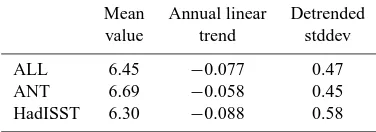
Table 1. Statistics of September ice extent time series in the ALL & ANT ensembles and in HadISST observations, from 1979–2012. All values are in millions of square kilometres.
Mean Annual linear Detrended value trend stddev ALL 6.45 −0.077 0.47 ANT 6.69 −0.058 0.45 HadISST 6.30 −0.088 0.58
formance of the ensembles in the period of satellite obser-vations, we compare the mean value, the linear trend, and the detrended standard deviation over the period 1979–2010, shown in Table 1. In mean value the ALL ensemble values match observations extremely well, and the ANT ensemble quite well. The linear trend of the ALL ensemble is quite close to that of observations, but a little too shallow; the lin-ear trend of the ANT ensemble is much too shallow. The detrended standard deviations are also similar, although the model has a slightly lower variability than observations.
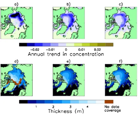
Fig. 2. (a–c) show linear trend in September ice concentration (yr−1) from 1979–2011 in the HadISST observations, and in the HadGEM1 ALL and ANT ensembles respectively. (d–f) show mean ice thickness from 1994–2000 in a superposition of satellite and submarine observations from that period (described more fully in Appendix A), and in the ALL and ANT ensembles respectively.
the ALL and ANT ensembles respectively. This effect would be likely to decrease concentration in the Atlantic (Pacific) sector sooner (later) than has been observed.
Having briefly evaluated the performance of the HadGEM1 ensembles up to the present, we now exam-ine its future projections. In Fig. 1a, the most surprising aspect of the time series post-2010 is a slowdown, even a temporary cessation, of sea ice loss projected in both ensembles. After 2030 ice loss appears to resume in the single continuing ensemble member. Note that the slowing is not apparent in the figures of Wang and Overland (2009), because they show only one ensemble member (ANT 1) in which the slowing is less severe than in many other mem-bers. In order to examine the rates of decline more closely, a 15-yr running gradient is plotted for each experiment, using the gradient of the least-squares linear fit to each 15-yr interval (Fig. 1b). The “flattening” is more clearly visible in the ALL ensemble than in the ANT; there is a clear minimum in the gradients in the late 1990s, followed by an increase to near, or above, zero at around 2010.
Formally, a shallowing of the decline is declared to be significant for any individual experiment if there exist two successive 15-yr periods for which the gradient intervals do not overlap. The gradient interval for any 15-yr period is defined as
gradient−2×(stderr) ,gradient+2×(stderr) , where stderr is the standard error in the linear fit to the 15-yr time series. Using this method, we find that the shallowing is significant in two out of the three ALL members continued to 2030 (ALL 3 & 4), and two out of the four ANT members (ANT 2 & 3). The same analysis is then carried out on the
September ice volume, a variable with less interannual vari-ability. The shallowing in this variable is significant for all of the above experiments (and in addition for ANT 1), demon-strating that there is a clear slowing of ice loss in many of the model runs, at similar times. As noted above, there is no clear cause for this slowing in the actual forcing of the runs, which varies continuously throughout the period of interest.
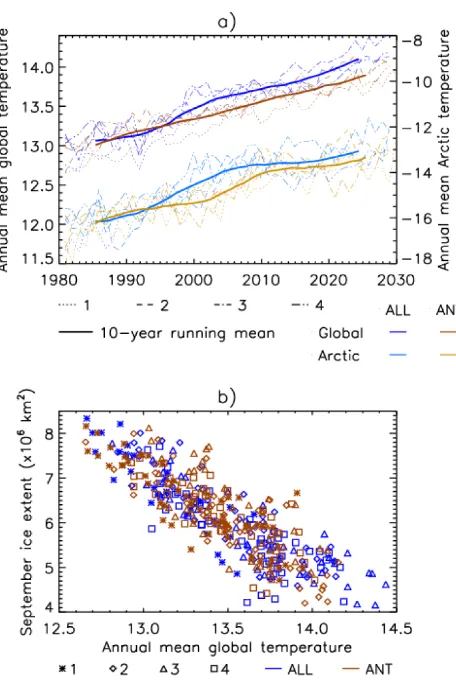
The time series of mean global temperature, and mean temperature north of 70◦N (“Arctic temperature”), are ex-amined, from 1980–2030, for the ALL and ANT experiments (Fig. 3a). Sea ice extent is also plotted against the global tem-perature (Fig. 3b) and Arctic temtem-perature (not shown). Arc-tic temperature varies roughly linearly with sea ice extent in all experiments; for example, in the experiment ALL 4 the time series rises to a maximum of−12.8◦C in the late 2000s, then decreases to−14.8◦C in the mid-2010s as ice extent in-creases, before slowly rising again. The behaviour of global temperature is more complicated, resulting in the large scat-ter apparent in Fig. 3b. Only one of the ANT experiments, ANT 3, displays a slowing of global temperature rise; by contrast, all three of the continuing ALL experiments show this. In ALL 2 & 3 the gradient minimum occurs in 2005 and 2011 respectively, but ALL 4 does not show a defined minimum, the temperature remaining roughly constant from 1999–2020. The magnitude of the slowing in global ature rise in these experiments is such that the Arctic temper-ature changes alone are not sufficient to explain them, which suggests the existence of other factors, external to the Arctic, which are helping to cause both.
Prior to 2010, the experiments have projected sea ice loss with reasonable accuracy, so here we analyse why the slow-down occurs, to identify the model processes responsible, and to assess the likelihood of the slowdown being observed in the real world.
3 Arctic heat budget
3.1 Methods and error evaluation
Fig. 3. (a) shows time series of global and Arctic temperature (mean temperature north of 70◦N) in the ALL and ANT ensem-bles; (b) shows annual mean global temperature (◦C) plotted against September mean ice extent (×106 km2).
therefore for these two components residual error terms are calculated and assessed. The methods used are described in more detail in Appendix B.
The heat budget allows easy comparison between the ice volume changes and the energy balance in the ice, because the ice component of the HadGEM1 model is “zero-layer”, effectively assuming the ice to have no heat capacity (al-though a very thin “skin layer” at the top is given a heat capacity to better simulate the diurnal cycle). Thus any ex-cess heat flux into the ice will simply melt the ice, while an energy deficit will cause a proportional amount of ice to be created. Ice volume and ice heat energy become effectively the same quantity, related by the constant−ρiceqice,ρice be-ing ice density andqicebeing specific latent heat of melting. Ice heat uptake is equivalent to ice volume loss, and “ice heat transport” into the Arctic is equivalent to advection of ice out of the Arctic Ocean region.
Fig. 4. Schematic to show how the Arctic heat budget was cal-culated. The bottom panel shows the Arctic Ocean as defined in Sect. 3. The western Arctic and eastern Arctic regions used in Sect. 3.3 are also shown.
3.2 Results
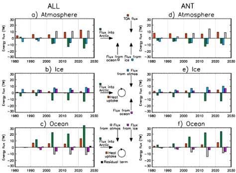
Decadal means of calculated fluxes for 1960–2030 are plot-ted in Fig. 5, showing the ensemble mean for the ALL and ANT experiments respectively. For each ensemble, the time mean value of each flux for the equivalent periods in the con-trol runs has been subtracted, to reduce the absolute values to similar magnitudes and enable the decade-to-decade changes to be more easily examined. In the discussion paragraphs be-low, the label “1980s” refers to decadal means from 1980– 1989, and similarly for all other decades. Note that fluxes are given in bulk (TW), so the changing ice area has no direct impact on the plotted quantities.
Fig. 5. Decadal means of terms in the Arctic heat budget for the ALL ensemble mean (a–c) and the ANT ensemble mean (d–f). For each term, the time mean of the equivalent periods in the control runs from 1980–2030 has been subtracted. The sign convention is that denoted by the arrows: positive inward for all fluxes. The colour scheme is the same as that used in Fig. 4.
the 1990s to the 2000s, there is little change in IHU, as in-creases in OI (2.08 TW) and AI (3.29 TW) are more than bal-anced by a very large decrease in ice heat transport (IHT) of 6.91 TW. This may be partly due to the ongoing ice loss it-self, as the ice flowing out of the Arctic Ocean will be ex-pected to be thinner. It appears likely from this discussion that the OI is the predominant driver, in the ALL runs, of the different rates of melting between 1980–2030, although the large drop in IHT after the 1990s also has some effect. We therefore next examine the ocean heat budget (Fig. 5c) to try and determine the causes of the changes in OI.
Ocean heat transport (OHT) rises steeply from the 1980s to the 2000s (increasing by 11.87 TW and then 10.61 TW from decade to decade), then decreases slightly by 1.93 TW into the 2010s. From the 1980s–1990s the large increase is mainly balanced by oceanic heat uptake (OHU), which rises by 6.58 TW; from the 1990s–2000s it is balanced by atmosphere-to-ocean flux (AO), which falls by 9.73 TW. The AO and ice-to-ocean (IO, equal and opposite to OI) fluxes are in fact consistently decreasing between the 1980s and 2000s. We conclude that the changes in OHT are entirely driving the changes in OHU, and are opposed by the changes in AO and IO; increased heat transport into the Arctic is resulting in ocean warming and increased heat flow to the atmosphere and ice. From the 1980s to the 1990s, the increase princi-pally causes ocean warming; from the 1990s to the 2000s, there is no increase in ocean warming, but instead greatly in-creased heat flow to the atmosphere, while ocean-to-ice flux increases throughout. From the 2000s to the 2010s, by con-trast, the OHT does not increase significantly, even reducing slightly, and hence the ocean-to-ice heat flux decreases as well.
In summary, the slowdown in ice melt in the ALL runs appears to be principally attributable to the slowdown in the increase of oceanic heat transport into the Arctic from the 2000s to the 2010s. However, the sharp decrease in ice trans-port from 1990s to the 2000s may also have had some effect, and would bear further investigation. It would also be inter-esting to examine whether, in the period of the slowdown, the ocean became less efficient at converting increased OHT to increased OI, via a strengthening of the halocline.
The ice heat uptake in the ANT experiments displays slightly different behaviour to that of the ALL experiments (Fig. 5e). Ice heat uptake begins from a fairly high value in the 1980s (1.18 TW). It displays a small decrease of 1.30 TW into the 1990s, a larger increase of 1.82 TW into the 2000s, and finally a large decrease of 3.10 TW into the 2010s cor-responding to the slowing of ice loss. This last decrease ap-pears to be entirely caused by a decrease in IHT (5.37 TW), with the flux terms from the atmosphere and the ocean actu-ally opposing the change, decreasing by 1.47 and 0.80 TW respectively. Advective effects are acting to slow ice loss, while thermodynamic effects are acting to increase it; in this short time period the advective effects are “winning”. The decrease from the 1980s to the 1990s appears to be caused by another decrease in IHT (2.52 TW), opposed by a rise in OI (1.91 TW); the increase from the 1990s to the 2000s was caused by a large increase in AI (2.60 TW), opposed by an-other small decrease in IHT (0.71 TW). In this experiment, the OI does not appear to be nearly as important as the IHT.
To summarise, the slowdown in ice loss shows clearly in the heat budget of both ensembles a drop in IHU from the 2000s–2010s. It is accompanied by steep drops in IHT in both ensembles, although the ALL IHT drop occurs a decade earlier than that of the ALL IHU. There is also a decrease in OI in the ALL ensemble, probably caused by the slow-down in the rise of OHT. Together, the heat budgets suggest the following questions: what causes the drop in ocean heat transport in the ALL ensemble, and why is a similar drop not observed in the ANT ensemble? Is this decrease the only rea-son for the decreased OI, or have changes in the Arctic Ocean mixed layer contributed? Why do the steep drops in ice heat transport occur, and why do they occur when they do?
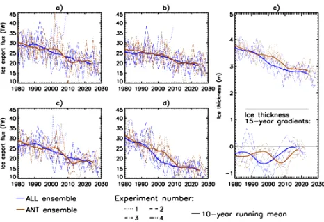
3.3 Changes in ice export
A decreasing trend in ice export from the Arctic is a fea-ture of all of the simulations. The ice transport in the ALL runs shows a short but fairly continuous period of decline (Fig. 6a), from about 30 TW in 1990 to about 23 TW in 2010. In the ANT runs, by contrast, there is a sharper decrease around 2010, from 27 TW to 20 TW. This decline is almost certainly playing a part in the slowing of ice loss. It could itself be caused by a decrease in the thickness of ice leaving the Arctic and/or a decrease in the speed of outflow.
Fig. 6. Ice export from the Arctic Ocean in the HadGEM1 runs. Showing (a) exact ice export as calculated in the heat budget; (b) ice export through the Fram Strait, calculated as∫hicevice·dS; (c) ice export calculated as in (b), but with the time-varying vicefields re-placed by their time mean; (d) ice export calculated as in (c), but with thehicefields replaced by their time mean, plus the time series of anomalies of ice thickness in the western Arctic region as defined in Fig. 4. (e) shows mean ice thickness in the western Arctic region, with 15-yr running gradients.
accurate answer, but it is difficult to analyse further. Ice ex-port can also be calculated asRhicevice·dS, wherehice and vicedenote ice thickness and velocity respectively, andSis the Arctic Ocean boundary. This is less accurate, as monthly mean fields ofhiceandvicemust be used, and variations in export due to correlations between the two quantities conse-quently lost, but allows easier investigation. To examine the relative effects of thickness and velocity on the transport time series, the ice heat transport across the Fram Strait is calcu-lated in this way, holding the ice thickness (velocity) fields constant, using the time mean field, in order that only the ice velocity (thickness) is varying in time.
There is no qualitative change to the patterns observed when ice export was calculated asRhicevice·dS; the same patterns of decline for both ensembles are observed (Fig. 6b). The same is true when the velocity fields were replaced by the time mean (Fig. 6c). However, when the thickness fields were replaced by the time mean, the pattern changes com-pletely, and ice transport actually increases in every run over the period 1960–2030 (not shown). From this it can be con-cluded that the changes in ice transport are entirely due to decreases in the thickness of the ice arriving at the boundary, and increased ice velocity is acting to oppose this slightly. This does not immediately rule out a change in atmospheric circulation as a cause; more ice could for example be being advected from the eastern Arctic after 2010, a region of gen-erally divergent, and therefore thinner, ice.
Two sub-regions of the Arctic adjacent to the Fram Strait are identified: the region between 120–0◦W , north of 79◦N, known hereafter as the “western Arctic” (WA), and the
re-gion between 0–120◦E north of 79◦N, known hereafter as the “eastern Arctic” (EA). In order to attribute the decline in Fram Strait ice transport to (a) changes in ice thickness in the WA, (b) changes in ice thickness in the EA, and (c) changes in the proportion of ice coming from each region, mean ice thickness in the whole Arctic Ocean (AO), WA and EA is plotted for each ensemble, and for each ensemble mean, from 1960–2030, and 15-yr gradients are calculated.
The gradients of ice thickness change in the WA show pro-nounced minima in the late 1990s and late 2000s for the ALL and ANT ensembles respectively, indicating step decreases in WA ice thickness at these times (Fig. 6e). The gradients of change of AO and EA ice thickness (not shown) also show minima close to these times, but these are higher and closer in value to the rest of the gradient time series. The step de-creases in WA ice thickness occur, in both ensembles, imme-diately before the steepest decrease in ice export; it is there-fore likely that this decrease is the most important cause of the ice export decrease.
As a second check, the ice export is calculated again as ∫hicevice·dS; the velocity at the boundary is again replaced by the time mean field, but the thickness at the boundary is also replaced by the time mean field plus the time series of anomalies in WA ice thickness. Very similar patterns in ice export are seen (Fig. 6d), but exaggerated and shifted ear-lier in time; a step change from ∼23 to ∼15 TW is seen in the late 2000s in the ANT runs, with a slightly steadier decrease being observed in the ALL runs during the 1990s, from∼28 to∼15 TW. This suggests that the changes in WA ice thickness are accounting for the changes in ice export, but that there is a time delay and that the effects are ameliorated somewhat by ice transport from other areas of the Arctic.
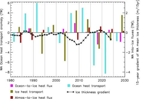
Fig. 7. The heat budget analysis for the western Arctic region, shown for the ANT 1 run, with a time series of the ANT 1 ice thick-ness gradient superimposed. Notice that the ocean heat transport is shown on a smaller scale (left) than that of the into-ice variables (right).
A similar event is in fact observed in the long control run of HadGEM1, in which forcing is kept constant at pre-industrial values (note that in the control run year numbers are arbitrary, and do not reflect any particular historical forc-ing). In year 1990 a flushing event removes a large amount of ice from the WA region; the 12-month running mean ice volume decreases from 1.05×10¹³m3 in late 1989 to 8.55×10¹²m2in late 1990, a decrease which energy bud-get analysis shows to be entirely ice export-driven. Starting in late 1990, however, there is a systematic decrease of ice export from the Arctic Ocean, resulting in a strong increase of Arctic Ocean ice volume; the 12-month running mean vol-ume increases from 3.18×10¹³m3in late 1990 to a peak of 3.52×10¹³m3in mid-1995, remaining at elevated levels for the rest of the 1990s. The appearance of such an event in the control run, together with those in the forced runs, sug-gests that sharp variations in ice thickness in the WA region are in HadGEM1 a common mechanism for causing vari-ations in Arctic ice volume on timescales of 2–10 yr. The slowdowns seen in the forced runs, therefore, may be at least partly caused by the fast ice losses of∼10 yr previously be-ing disproportionately concentrated in the WA region.
3.4 Changes in ocean heat transport and in the Arctic Ocean mixed layer
In HadGEM1, the principal source of heating of the Arctic Ocean by water transport is from the Atlantic Ocean, through Fram Strait and the Barents Sea. The rate of heating from the Atlantic is controlled by the temperature of the water at inflow, and the speed of inflow. To examine the relative ef-fects of these terms, a similar analysis to that in Sect. 3.3 was performed: the oceanic heat transport OHT=RTocnuocn·dS was re-calculated twice,Tocnanduocnbeing held constant in
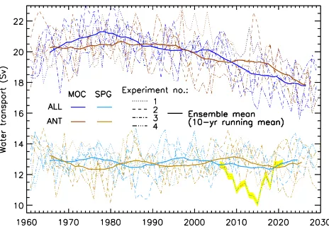
Fig. 8. Ocean heat transport into the Arctic Ocean in the HadGEM1 runs. Showing (a) OHT= ∫Tocnuocn·dS, as calculated in the heat budget; (b) as in (a), with velocity fields replaced with the time mean; (c) as in (a), with temperature fields replaced by the time mean. Each figure shows ocean heat transport (top sets of lines, left scales) and 15-yr running gradients (bottom sets of lines, right scales).
turn by replacing each term by its respective time mean field. Tocnanduocnare ocean temperature and current velocity re-spectively, andSis the Arctic Ocean boundary.
Figure 8 shows OHT as calculated in each of these three ways. Figure 8a shows OHT as in the heat budget, with time-varying temperature and velocity; in the ALL runs we see a steep rise in OHT from the late 1980s, checked and briefly reversed in the mid-2000s, and resuming from about 2020. There is variation within the ensemble; OHT is reversed most strongly in ALL 4, but checked hardly at all in ALL 3. The ANT ensemble displays a very similar pattern, shifted 7–8 yr into the future. These patterns are to a large degree repli-cated when the velocity field is replaced by the time mean (Fig. 8b); however, when the temperature field is replaced by the time mean (Fig. 8c), the time series becomes virtu-ally flat, although there are still weak falls in OHT around the time of the reversals. This suggests that the water flow-ing into the Arctic is warmflow-ing, then coolflow-ing, then warmflow-ing again, and that around the time of the reversals there is also a slight reduction in the into-Arctic current velocities.
To seek an explanation for these effects in turn, we exam-ine two important aspects of the North Atlantic circulation: the meridional overturning circulation (MOC) and the sub-polar gyre (SPG). We define the strength of the MOC in the usual way, as the maximum overturning stream function in the North Atlantic. The SPG is more complex to define as there are two separate cyclonic gyres in the North Atlantic, in the Labrador Sea and in the Nordic seas. We concentrate on the Nordic gyre as it influences conditions at the Arctic– Atlantic boundary more directly, and define its strength to be the maximum gyre stream function between 66–80◦N.
Fig. 9. Variation of the MOC (dark colours, top set of lines) and the subpolar gyre (light colours, bottom set of lines) in the HadGEM1 experiments. The SPG index of ALL 4 has been highlighted from 2006–2021.
ensemble exhibits a step decrease at around 2008, but in the ANT ensemble the decrease is more gradual. The distribu-tion of the ALL MOC indices in the period (1993–2007) was compared to that in the period (2008–2023). The initial pe-riod has mean index 20.1 and spread 0.8: the later pepe-riod mean 18.5 and spread 1.2. The distributions are significantly different at the 5 % confidence level; i.e. there is a signif-icant weakening of the MOC in 2008 of around 1.6 Sv. A decrease in the MOC index would be expected to have a substantial negative effect on the ocean temperature at the Arctic–Atlantic boundary; therefore it is likely that this step decrease is a major cause of the changes.
In the SPG index there is no systematic decrease. How-ever, in ALL4 a short-term weakening is visible, with a min-imum in 2015 of 2–3 Sv below the long-term mean. Interest-ingly, there is a similar short-term weakening in ALL2 in the late 1980s which also coincides with a period of relatively high ice extent (Fig. 1) and low OHT (Fig. 8). There is in general no correlation between SPG index and September ice extent, but in the two cases mentioned above low SPG index coincides with low temperatures in the top 70 m of the Nordic seas, low OHT, low Arctic OI heat flux and high September ice volume as well. It is therefore reasonable to assume that while the SPG is not in general a major factor influencing sea ice, in these cases long periods of an extremely low in-dex are causing greater sea ice cover than would otherwise be the case. While changes in the SPG index cannot there-fore explain the slowing of ice loss across the ensemble, it may explain why the slowing is most pronounced in ALL 4. The MOC changes in particular may help to partly ex-plain the behaviour in global temperature time series seen in Sect. 2. The sharp change in the MOC in the ALL runs in late 2008, with the concurrent stable Arctic sea ice and Arctic temperatures, may have helped to keep global temperatures at a roughly constant level for several years (although as for
ALL 3 & 4 the “flattening off” of global temperatures oc-curred around 2000, this was probably not the only factor). The more gradual decline in the MOC in the ANT runs is consistent with the more constant rate of temperature rise in this ensemble.
We now briefly discuss the behaviour of the mixed layer in the ALL 4 integration, as this is the run displaying both the most prominent ice loss slowdown and the most dramatic changes in ocean circulation. The annual mean salinity of the mixed layer (defined to be the top 50 m) of the Arctic Ocean was plotted for years 1980–2030 of this run (Fig. 2 of reply to Referee 2). The salinity is consistently decreasing throughout this period, but the decrease is slowest in the 1990s, when the ice loss is fastest, and is fastest in the early 2010s, when the ice loss is slowest, which suggests that in this run a rapid freshening of the mixed layer is inhibiting ocean heat from influencing the ice, and thus assisting the slowing of ice loss. A freshwater budget of the Arctic Ocean (without ice) was computed for this run to determine causes for these gradi-ent changes, and it was seen that the freshening of the early 2010s was caused almost entirely by an increase in freshwa-ter transport through the Bering Strait. This freshwa-term displays a large, systematic change during the period of interest, rising from∼2000 km3yr−1in the late 1990s to∼3000 km3yr−1 in the early 2010s, and falling back again to∼2000 km3yr−1 in the mid-2020s. Through the 2010s and 2020s, the fresh-water “import” through the Fram Strait displays a decrease of similar magnitude, indicating increased export of fresh-water, corresponding to an abrupt slowing of the fall in salin-ity, and probably reflecting “flushing” of freshwater from the Arctic Ocean. A marked freshening of the Nordic seas is in-deed visible during the 2010s. This may in turn have helped depress the MOC index throughout the 2010s and 2020s, as seen above.
The contribution from ice melt/formation dominates the interannual variability of the freshwater budget on short timescales, probably reflecting interannual variability of ice export, but has a little consistent signal on longer timescales; it is therefore unlikely that the long-term changes in ice melt are significantly affecting the salinity of the Arctic Ocean mixed layer.
A detailed analysis of the causes of the anomalous Bering Strait freshwater import is beyond the scope of this paper. A freshening of the North Pacific from the mid-2000s to the 2010s is seen, but the causes of this are hard to determine.
4 Discussion
temperature is simulated at a similar time to the slowing of ice loss.
In this paper, three principal mechanisms have been iden-tified as being responsible for this slowdown, two closely re-lated. Firstly, there is the weakening of the MOC, which ap-pears to reduce (or slow the rise of) the heat flowing into the Arctic Ocean, and hence reduce the ocean to ice heat flux. The weakening is sudden in the ALL ensemble, occurring at around 2008; it is slower, and about a decade later, in the ANT ensemble, and thus goes some way towards explaining the difference in timing of the slowdown between the two ensembles. It may also be partially responsible for the halted rise in global temperatures. In addition, a marked weakening of the SPG and freshening of the Arctic Ocean mixed layer have been identified in ALL 4, the run displaying the most severe slowdown.
Secondly, there is the negative ice export feedback iden-tified, whereby a thinning ice cover will reduce the rate at which ice is exported from the Arctic. Ice loss in the ALL experiments reaches its maximum rate in the late 1990s (Fig. 1b). Most of the ANT experiments do not display clear minimum gradients of ice loss, but ANT 3 displays a similar gradient minimum in the early 2000s. All of these experi-ments then display similar rates of rise in gradient as ice loss slows. The negative ice export feedback would be expected to begin to take effect 3–7 yr after the gradient minima, based on the average residence times for ice in the Arctic. There-fore, the timing of fastest loss may also provide an explana-tion as to the differing times of the slowdown. Whether the value of the steepest rate of change affects the strength of this feedback is not clear.
Lastly, there are the sudden decreases in ice thickness in the region immediately north of Greenland, in the late 1990s and late 2000s in the ALL and ANT ensembles respectively, which together with the effect above appear to precipitate the sudden declines in ice export from the Arctic in around 2000 and 2010 respectively. Clearly these are related to some ex-tent to the time of fastest total ice loss, but other than this their cause is difficult to determine. In some experiments “flushing” events appear to play a role. In others, temporary periods of increased oceanic heat convergence to this region appear to be responsible.
Do we expect any of these effects, and a consequent slow-ing of ice loss, to be observed in the near future? A slowslow-ing of the MOC during the 21st century is widely projected to occur by climate models, as a result of warming and freshening of the North Atlantic. However, this is likely to lead to a smaller slowing of ice loss than that projected in HadGEM1, for the reasons detailed in Sect. 2: while in HadGEM1 regions of present-day ice loss are spread fairly evenly around the edge of the Arctic, in observations the region of ice loss is strongly concentrated in the Pacific sector. We would therefore expect ice loss to be less strongly affected by changes in the At-lantic. It has also been found that a decreasing MOC will not necessarily decrease OHT into the Arctic Ocean (Bitz et
al., 2006) as in HadGEM1 the centres of overturning tend to move north in the long term, closer to the Arctic–Atlantic boundary.
The SPG changes observed in ALL 4 appear to be a freak event, as they are not seen in other runs, while the changes in Bering Strait freshwater import are quickly reversed; there therefore appears no particular reason to suppose that these will be observed in reality. Freshening of the Arctic Ocean mixed layer by direct ice melt may be important in suppress-ing further ice melt on interannual timescales, but probably not on the rather longer timescales discussed in this study.
The negative feedback of ice export is almost certainly a real effect which has been already acting to retard ice loss slightly (relative to the loss that would have been observed with a constant rate of ice export). Nevertheless, it is un-likely that the feedback could on its own slow ice loss as time progresses. This can be shown using a simple box model of the Arctic, evolving ice volume and ice export rate in time (described in Appendix C). Ice loss could probably only be briefly slowed by short periods of fast ice loss in certain parts of the Arctic, as described above. A series of studies (e.g. Ogi et al., 2010; Ogi and Wallace, 2012) have examined the role of advective sea ice loss in driving September minima, no-tably the recent low ice events, and identify a clear role for sea ice export to affect ice extent on shorter timescales. How-ever, their findings relate to the sea ice export changes that are driven by atmospheric circulation, rather than a thinning ice cover.
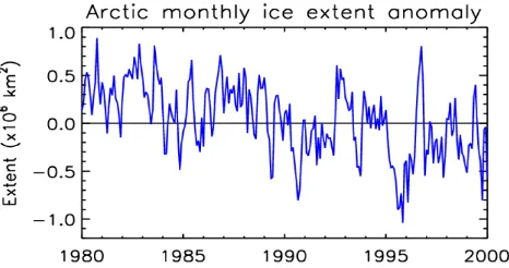
The causes of the sudden ice losses north of Greenland are too varied and complex for the likelihood of their occurring in the real world to be easily assessed, although increased ocean heat convergence has been found to be important in causing Arctic-wide rapid ice loss events in other models beside HadGEM1 (Holland and Bitz, 2006). The “flushing” events seen in some simulations, and in the control run, sug-gest that, following these, total ice loss may for some time continue at a slower rate than that which was occurring be-fore the event. A close precedent for this may have actually occurred in the early 1990s. It is generally believed that a sudden increase in the Arctic Oscillation index around 1989– 1990 resulted in a large amount of thick multi-year ice being expelled from the Arctic (Rigor and Wallace, 2004; Rothrock et al., 2003), and about this time there appears to be a local minimum in ice extent in all months. However, in the fol-lowing years ice extent increased again, recovering to 1980s levels by 1995, whereupon another sharp decrease occurred (Fig. 10). Reduced ice export from the western Arctic region may have helped in this temporary recovery. It would be the-oretically possible for this mechanism to temporarily slow ice loss at any point in the future, albeit probably for a shorter time period than is seen in the HadGEM1 experiments.
Fig. 10. Time series of monthly mean Arctic sea ice extent anoma-lies from the HadISST dataset, 1981–2000. Anomaanoma-lies are taken relative to the 1981–2000 mean extent for each respective month.
model has provided clues as to what mechanisms might be causing a slowdown, with one to be observed at any point in the future.
Appendix A
Combining satellite and submarine observations of ice thickness in one figure
A1 Description of datasets
The spatial pattern of mean ice thickness from 1994–2000 shown in Fig. 2d is derived from two datasets: (i) a multiple regression of moored upward-looking sonar submarine mea-surements of ice draft (Rothrock et al., 2008) and (ii) gridded measurements of ice thickness from satellite radar altime-try (Laxon et al., 2003). The submarine observations cover a large area of the central Arctic known as the SCICEX box, including the North Pole; the satellite observations cover the area south of 81.5◦N. Together they cover much of the Arc-tic Ocean. The figure was produced for illustrative purposes only and is not itself a new dataset; due to the very differ-ent nature of the two sources, it should be used with great caution.
The two datasets, in their raw form, represent different quantities. The submarine data, obtained via the formula given in Rothrock et al. (2008), are effectively gridbox mean ice draft (including open water areas). To convert to gridbox mean ice thickness, the field was multiplied byρwater
ρice , the ra-tio of water and ice densities. The satellite data, however, are in the form of mean ice thickness not including thin ice and open water. “Thin ice” is defined by Laxon et al. (2003) as ice thinner than 0.5 to 1 m. It was necessary to carry out a transformation on this field, based on the HadISST ice con-centration data and described below, to convert it to approxi-mate gridbox mean ice thickness.
A2 The “thick ice” to “gridbox mean ice” transformation
LetH1 denote mean thickness of “thick ice”, as in the raw dataset,γ ice concentration,HMOI mean ice thickness over ice (i.e. not including open water), andHGBMgridbox mean ice thickness. We say thatH1is mean thickness of ice greater thanηmetres thick, knowing that 0.5≤η≤1. Letg(h)be the ice thickness distribution function, and assume that, for 0< h≤η, ice growth rate is inversely proportional to ice thickness (ddht =c
h), and thatg(h)∝ 1 dh dt
(i.e. distribution den-sity at h is inversely proportional to rate of growth at h). Theng(h)=g1h, some constantg1, for 0< h≤η. Assume that, for high concentrationγ,g1is inversely proportion to HMOI:
HMOI= 1 λg1
. (A1)
Then HGBM=
∞ Z
0
hg (h) .dh= η Z
0
g1h2.dh+ ∞ Z
η
hg (h) .dh
= 1
3g1h 3
η
0 +H1
∞ Z
η
g (h) .h
⇒γ HMOI= 1 3g1η
3+H 1 γ− η Z 0
g1h.dh
⇒ γ
λg1 =1
3g1η 3+H
1
γ− 1
2g1h 2
η
0
=g1η2 η
3− H1
2
+H1γ
⇒g21η2λ η
3− H1
2
+H1γ λg1−γ=0. (A2) This quadratic in g1solves to give
g1=
−λH1γ± r
(λH1γ )2+4γ λη2 η
3− H1
2
2λη2η 3−
H1 2
. (A3)
We take the “+” solution as it allowsg1→0 asH1→ ∞; intuitively we would expect the proportion of thin ice to be small for large H1. For the quantity inside the square root to be positive, λ≥ 4η2
γ
1 2H1
− η
3H2 1
is sufficient; and for H1≥1,η∈[0.5,1],λ≥43γ is sufficient. If we restrictγ≥12, then we can setλ=2 for simplicity.
So for 0.5≤γ≤1, we say
g1=
−2H1γ+ r
4(H1γ )2+8γ η2 η 3− H1 2
4η2η 3−
H1 2
For 0≤γ≤0.5, we try
g1=γ−α (H1) γ2, (A5)
so that for smallγ almost all ice is thinner thanη. The func-tions must match up atγ=0.5; therefore
α (H1)=2+ H1−
r
H12+4η2η 3−
H1 2
η2η 3−
H1 2
. (A6)
So g1(H1, γ , η) can be calculated for all values of γ and H1, obtained from the HadISST dataset and the Laxon et al. (2003) dataset respectively, using Eqs. (A6) and (A7). Then
HGBM=g1η2 η
3− H1
2
+H1γ , (A7)
as in Eqs. (A3) and (A4). For four sample months,HGBMwas calculated forη=0.5,0.6,0.7,0.8,0.9,1.0, and the result-ing fields compared. The largest difference inHGBMbetween these different options was 28.2 cm. For the final calculation, η=0.75 was used.
A3 Producing the figure and discussion of error
For Fig. 2d, the transformed fields were plotted together; where a gridbox contained data from both fields, a simple mean was used. The field is a time mean of all months from January 1994 to December 2000; in order to reduce the bias of missing summer months in the satellite field, grid points were filled in using the mean March ice thickness value with the seasonal cycle in ice thickness found by Rothrock et al. (2008) added (but cut off at 0 m). There are obviously large errors associated with both fields; for the satellite field these stem from the following: (i) uncertainty in the value of η; (ii) the assumptions leading to the equationg(h)=g1h for thin ice; (iii) incomplete coverage of certain areas for some months of the year. For the submarine field the errors principally stem from the multiple regression itself; they are discussed in Rothrock et al. (2008), who estimate the stan-dard deviation of variation not explained by their model to be 25 cm. For the (transformed) satellite field the errors will be larger still, hence the need for the figure to be used for illustrative purposes only.
Appendix B
How the Arctic heat budget was calculated
B1 Vertical fluxes
The vertical fluxes were calculated directly from diagnostics; all are positive downwards.
Top-of-atmosphere flux is calculated as follows:
TOA=SWdown−SWup−LWup, (B1)
where SWdowndenotes downward shortwave radiation at the top of the atmosphere, and similarly for SWupand LWup.
Atmosphere-to-ocean heat flux is calculated as follows: AO=(penetrating solar flux)+(htn) , (B2) where “htn” is a diagnostic representing all non-solar fluxes from atmosphere to ocean.
Atmosphere-to-ice heat flux is calculated as follows: AI=topmelt+chf+qice(sub-snow) , (B3) whereqiceis the specific latent heat of melting, “topmelt” the top melting heat flux, “chf” the conductive heat flux through the ice (from the atmosphere to the bottom surface), and “sub” and “snow” heat fluxes due to sublimation from and snowfall onto the ice respectively.
Ocean-to-ice heat flux
OI=ocnmelt+frazil+misc, (B4)
where “ocnmelt” denotes diffusive ocean-to-ice heat flux, “frazil” heat flux due to frazil ice formation, and “misc” small “correction” terms that pass heat between the ocean and ice when ice disappears, and when snow falls into the ocean during ice ridging.
B2 Horizontal fluxes and heat uptake
The horizontal transports into the Arctic are more difficult to compute. The atmospheric heat transport (AHT) into the Arctic was computed as a residual (AHT=AO+AI−TOA), assuming that the atmospheric heat uptake was negligible.
The ice heat transport and uptake (IHT, IHU) were calcu-lated using “rate of change” diagnostics:
IHT=qice ρice Z
dhice
dt
dyn
.dA+ρsnow Z
dhsnow
dt
dyn .dA
!
(B5)
IHU=qiceρice Z d
hice dt dyn + d hice dt therm + d hice dt ridge !
.dA
+qiceρsnow Z dhsnow dt dyn + dhsnow dt thermo + dhsnow dt ridge !
.dA,(B6) whereρice is ice density,hice gridbox mean ice thickness; ρsnowandhsnoware the analogous quantities for snow.t de-notes time. The subscripts “dyn”, “therm” and “ridge” indi-cate rates of change of ice and snow thickness due to advec-tion of ice, thermodynamic processes, and ridging processes respectively.
The oceanic heat transport (OHT) was calculated as OHT=
Z
Tocnuocn.dS, (B7)
In order to compute the heat uptake of the ocean (OHU), the annual mean heat content was computed first:
OHC=ρwatercwater Z
Tocn.dV , (B8)
whereρwaterandcwaterare sea water density and specific heat capacity at constant pressure respectively.
The heat uptake for any given year was then calculated to be
OHU(t )=OHU(t+1)−OHU(t−1)
2 . (B9)
While this is obviously a very inaccurate method of calcu-lating year-on-year heat uptake, the long-term trends in heat uptake will be captured. It is very difficult to compute the exact heat uptake in the ocean for a given year using annual mean diagnostics. While monthly mean ocean temperature diagnostics were available, it was chosen not to use these for reasons of data storage and computational time, and be-cause annual mean data were considered sufficient to com-pute decadal means.
B3 Residuals
To evaluate errors in the calculation, a “residual” term can be calculated for each of the atmosphere, ice, and ocean – the energy entering the system that is left over, and does not appear in the heat uptake.
Atmospheric residual error=TOA+AHT−AI−AO Ice residual error=AI+IHT−IO−IHU
Ocean residual error=AO+IO+OHT−OHU Because the atmospheric heat transport into the Arctic is itself defined as the residual of the other terms, this was zero in the atmosphere component. It was extremely small in the ice component (∼O(1 GW)) due to the accuracy of the meth-ods used for calculating the into-ice fluxes. The methmeth-ods used for calculating OHU and OHT are less accurate; the residual was therefore of significant size, and is plotted in Figs. 5c and 4f with the other ocean fluxes.
Appendix C
A model of the ice export negative feedback effect
We say the Arctic containsV (t )cubic metres of ice at any timet, and that volume changes according to advective and thermodynamic effects. Specifically,
dV
dt = −µV+λ (V0−V ) (C1)
where−µV andλ (V0−V )represent ice volume change due to advective and thermodynamic effects respectively, andλ
andµare positive constants. Thus ice export is directly pro-portional to ice volume, and thermodynamic effects act to “push” ice volume towards a valueV0in which the ice is in thermodynamic equilibrium. Eq. (C1) solves easily to give an exponential solution in whichV approachesV0·λ+µλ , the “steady-state” volume.
We now simulate a constant rate of ice melt by replacing λ (V0−V ) withλ V0 1−Tt
−V in Eq. (C1), such that the “thermodynamic equilibrium volume” decreases linearly fromV0to 0 in timeT, and require thatV (0)=V0·λ+µλ , the steady-state volume at timet=0. This also solves exactly to give
V (t )=V0· λ λ+µ·
1− t T +
1 T (λ+µ)·
1−e(−(λ+µ)t )
.(C2)
Thusd2V dt2 = −
λV0
T ·e(−(λ+µ)t ), which is always negative, and the rate of ice loss never slows.
Acknowledgements. This study was supported by the Joint
DECC/Defra Met Office Hadley Centre Climate Programme (GA01101).
Many thanks to Jeff Ridley and Richard Wood for helpful sugges-tions and correcsugges-tions prior to submission.
Edited by: D. Feltham
References
Bitz, C. M., Gent, P. R., Woodgate, R. A., Holland, M. M., and Lindsay, R.: The influence of sea ice on ocean heat uptake in response to increasing CO2, J. Climate, 19, 2437–2450, 2006. Francis, J. A., Chan, W. H., Leathers, D. J., Miller, J. R., and Veron,
D. E.: Winter Northern Hemisphere weather patterns remember summer Arctic sea ice extent, Geophys. Res. Lett., 36, L07503, doi:10.1029/2009GL037274, 2009.
Hibler, W.: A dynamic thermodynamic sea ice model, J. Phys. Oceanogr., 9, 817–846, 1979.
Holland, M. M., Bitz, C. M., and Tremblay, B.: Tremblay, Future abrupt reductions in the Arctic summer sea ice, Geophys. Res. Lett., 33, L23503, doi:10.1029/2006GL028024, 2006.
Hunke, E. C. and Dukowicz, J. K.: An Elastic-Viscous-Plastic Model for Sea Ice Dynamics, J. Phys. Oceanogr., 27, 1849–1867, 1997.
Johns, T. C., Durman, C. F., Banks, H. T., Roberts, M. J., McLaren, A. J., Ridley, J. K., Senior, C. A., Williams, K. D., Jones, A., Rickard, G. J., Cusack, S., Ingram, W. J., Crucifix, M., Sexton, D. M. H., Joshi, M. M., Dong, B.-W., Spencer, H., Hill, R. S. R., Gregory, J. M., Keen, A. B., Pardaens, A. K., Lowe, J. A., Bodas-Salcedo, A., Stark, S., and Searl, Y.: The new Hadley Centre Cli-mate Model (HadGEM1): Evaluation of coupled simulations, J. Climate, 19, 1327–1353, 2006.
Laxon, L., Peacock, N., and Smith, D.: High interannual variability of sea ice thickness in the Arctic region, Nature, 425, 947–950, 2003.
McLaren, A. J., Banks, H. T., Durman, C. F., Gregory, J. M., Johns, T. C., Keen, A. B., Ridley, J. K., Roberts, M. J., Lip-scomb, W. H., Connolley, W. M., and Laxon, S. W.: Evaluation of the sea ice simulation in a new coupled atmosphere-ocean climate model (HadGEM1), J. Geophys. Res., 111, C12014, doi:10.1029/2005JC003033, 2006.
Ogi, M. and Wallace, J. M.: The role of summer surface wind anomalies in the summer Arctic sea ice extent in 2010 and 2011, Geophys. Res. Lett., 39, L09704, doi:10.1029/2012GL051330, 2012.
Ogi, M., Yamakazi, K., and Wallace, J. M.: Influence of winter and summer surface wind anomalies on summer Arctic sea ice extent, Geophys. Res. Lett., 37, L07701, doi:10.1029/2009GL042356, 2010.
Overland, J. E. and Wang, M.: Large-scale atmospheric circulation changes are associated with the recent loss of Arctic sea ice, Tel-lus A, 62, 1–9, 2010.
Rayner, N. A., Parker, D. E., Horton, E. B., Folland, C. K., Alexan-der, L. V., Rowell, D. P., Kent, E. C., and Kaplan, A.: Global analyses of sea surface temperature, sea ice, and night marine air temperature since the late nineteenth century, J. Geophys. Res., 108, D144407, doi:10.1029/2002JD002670, 2003.
Rayner, N. A., Kennedy, J. J., Smith, R. O., and Titchner, H. A.: The Met Office Hadley Centre Sea Ice and Sea Surface Temperature data set, version 2, part 3: the combined analysis, in preparation, 2013.
Rigor, I. G. and Wallace, J. M.: Variations in the age of Arctic sea-ice and summer sea-sea-ice extent, Geophys. Res. Lett., 31, L09401, doi:10.1029/2004GL019492, 2004.
Rothrock, D. A., Zhang, J., and Yu, Y.: The arctic ice thick-ness anomaly of the 1990s: A consistent view from ob-servations and models, J. Geophys. Res., 108, C33083, doi:10.1029/2001JC001208, 2003.
Rothrock, D. A., Percival, D. B., and Wensnahan, M.: The decline in arctic sea-ice thickness: Separating the spatial, annual and in-terannual variability in a quarter century of submarine data, J. Geophys. Res., 113, C05003, doi:10.1029/2007JC004252, 2008. Semtner, A. J.: A model for the thermodynamic growth of sea ice in numerical investigations of climate, J. Phys. Oceanogr., 6, 379– 389, 1976.
Strey, S. T., Chapman, W. L., and Walsh, J. E.: The 2007 sea ice minimum: Impacts on the Northern Hemisphere atmosphere in late autumn and early winter, J. Geophys. Res.-Atmos., 115, D23103, doi:10.1029/2009JD013294, 2010.
Stroeve, J. C., Holland, M. M., Meier, W., Scambos, T., and Serreze, M.: Arctic sea ice decline: Faster than forecast, Geophys. Res. Lett., 34, L09501, doi:10.1029/2007GL029703, 2007.
Stroeve, J. C., Serreze, M. C., Holland, M. M., Kay, J. E., Maslanik, J., and Barrett, A. P.: The Arctic’s rapidly shrinking sea ice cover: a research synthesis, Climatic Change, 110, 1005–1027, 2012. Thorndike, A. S., Rothrock, D. A., Maykut, G. A., and Colony,
R.: The Thickness Distribution of Sea Ice, J. Geophys. Res., 80, 4501–4513, 1975.