P R I M A R Y R E S E A R C H
Open Access
Mixture models for gene expression
experiments with two species
Yuhua Su
1*, Lei Zhu
2, Alan Menius
2and Jason Osborne
3Abstract
Cross-species research in drug development is novel and challenging. A bivariate mixture model utilizing information across two species was proposed to solve the fundamental problem of identifying differentially expressed genes in microarray experiments in order to potentially improve the understanding of translation between preclinical and clinical studies for drug development. The proposed approach models the joint distribution of treatment effects estimated from independent linear models. The mixture model posits up to nine components, four of which include groups in which genes are differentially expressed in both species. A comprehensive simulation to evaluate the model performance and one application on a real world data set, a mouse and human type II diabetes experiment, suggest that the proposed model, though highly structured, can handle various configurations of differential gene expression and is practically useful on identifying differentially expressed genes, especially when the magnitude of differential expression due to different treatment intervention is weak. In the mouse and human application, the proposed mixture model was able to eliminate unimportant genes and identify a list of genes that were differentially expressed in both species and could be potential gene targets for drug development.
Keywords: Orthology, Drug development, Drug response prediction, Type II diabetes
Introduction Background
Pharmaceutical medicine is an industry with huge up-front investment for rewards that may or may not come years later. A complete drug development process, includ-ing drug discovery, preclinical research (on animals) and clinical trials (on humans), is lengthy, expensive, and risky. Determined by the US Food and Drug Administration (FDA) [1], the average total cost per drug development is about $1.9 billion. The typical development time is 10 to 15 years. The overall attrition rate of a drug com-pound from first-in-man to registration is approximately 80%–90% [2,3].
FDA [1] calls the preclinical and clinical research together as the ‘critical path’ development phase, where most investment required for a successful drug launch occurs. Currently, this development phase is inherently inefficient. The goal of preclinical research is to assess how a drug is absorbed, distributed, metabolized, and
*Correspondence: [email protected]
1Dr. Su’s Statistics & Department of Human Nutrition, Food, and Animal Sciences, University of Hawaii at Manoa, Honolulu, HI 96822, USA Full list of author information is available at the end of the article
excreted in animals, and to use the findings to deter-mine potential human outcomes before starting clinical trials. Yet the rate of success after a drug candidate enters Phase I is undesirably low. As mentioned in FDA [1] and Kola and Landis [3], animal models with poor clinical relevance may be accountable for this perplex-ity. Hence, improving translation between two species to increase the predictive power of animal models to human studies is of tremendous value to drug discovery and development.
Homology and multiple species gene expression analysis in drug development
Microarrays are tools for gene expression analysis and can be potentially useful for investigating the mechanism of drug activities that translates across species. The util-ity of microarray information in the drug development process is reviewed by Braxton and Bedilion [4] who embraced the idea that gene expression analysis can be a surrogate marker for the interaction between compounds and cells and should yield information about efficacy. Debouck and Goodfellow [5] believed that microar-rays can be used to generate clues to patterns of gene
function that can help improve the efficiency of drug development.
As stated before, one key challenge of drug develop-ment is to successfully translate the results of preclinical findings in animal models to human beings in the clinic. Pre-clinical experiments assume that the effect of the drug tested on animals is comparable to that on humans, which can only be true if a functional equivalent of the human drug target exists in the experimental species. Orthol-ogy [6-8] is a strong indication of functional conservation and therefore provides the best functional annotation of experimentally undetermined genes across species. Holbrook and Sanseau [9] remarked that the use of orthologs has the potential to improve the understand-ing of biological differences between species (animals and humans).
Many of the successful applications of cross-species microarray gene expression analysis involve orthology [10-13]. Additionally, over the past decade, researchers have tried to use orthology and gene expression data to do cross-species comparison in order to understand how genes interact to perform particular biological processes [14,15]. These studies support the idea that orthologs could be a useful tool for researchers to link experiments between species in drug development. Note that orthol-ogous relationships can be one-to-one, one-to-many, or many-to-many [8].
The rest of the paper is structured as follows: Section ‘Joint modeling across species’ describes the proposed bivariate mixture model across species. Section ‘Simulation’ describes a simulation study under-taken to investigate the effects of different experimental designs on the power to detect important genes and on misclassification rates. Section ‘Application: the mouse and human type II diabetes experiment’ illustrates the methodology using an application to data collected in a mouse/human experiment. Section ‘Concluding remarks’ concludes.
Joint modeling across species
Let Xaij and Xhil denote gene expression measurements from theith orthologous gene pair for thejth animal and the lth human. The following independent linear mod-els describe the association between gene expression and treatment:
Xaij = β0ai+β1aiTaj+eaij, (1)
Xhil = β0hi+β1hiThl+ehil, (2)
where Taj and Thl are {0, 1} treatment indicators, and eaij andehil are independentN(0,σ
2
a) andN(0,σh2)
ran-dom variables.σa2 andσh2are variances for eaij andehil,
respectively. In drug development, the animal research and human experiments are conducted independently -one’s results do not affect the other’s. However, the treatment effects are expected to have some kind of association between the two species. This results in our choice of using two independent models for the two species to capture the effects of treatment on gene expression.
A nine-component bivariate mixture model for two species experiments
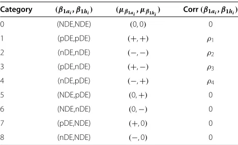
β1ai andβ1hi quantify the differential expression of the ith orthologous animal and human genes due to a treat-ment intervention. A given gene can be classified as non-differentially expressed (NDE) - showing no signs of treatment effects, positively differentially expressed (pDE) - showing positive treatment effects, or negatively differentially expressed (nDE) - showing negative treat-ment effects. Therefore, for a human and animal gene pair, there are nine possibilities for categorizing this pair of genes. Further, dependency is assumed between differentially expressed orthologs, i.e., existence of asso-ciation posited only for (β1ai,β1hi)
T in categories (1,
2, 3, 4) and zero correlation presumed for (β1ai,β1hi)
T
in categories (0, 5, 6, 7, 8). Table 1 illustrates the nine possible categories of (β1ai,β1hi)
T. (μ
β1ai,μβ1hi)
T is the
vector of population means of (β1ai,β1hi)T under each category.
In consequence of these possible patterns of (β1ai,β1hi)
T, mixture models [16,17] are adopted to deal
with the correlation and distribution of each subgroup of genes across species. An additional advantage of mixture models is that, after prior weights for the components are specified, estimates of the posterior probabilities of population membership can be formed for each obser-vation to give a probabilistic clustering. As a result, the pooling of information for genes across species can be exploited to better understand the underlying
rela-Table 1 Possible categories of(β1ai,β1hi) T
Category (β1ai,β1hi) (μβ1ai,μβ1hi) Corr(β1ai,β1hi)
0 (NDE,NDE) (0, 0) 0
1 (pDE,pDE) (+,+) ρ1
2 (nDE,nDE) (−,−) ρ2
3 (pDE,nDE) (+,−) ρ3
4 (nDE,pDE) (−,+) ρ4
5 (NDE,pDE) (0,+) 0
6 (NDE,nDE) (0,−) 0
7 (pDE,NDE) (+, 0) 0
tionship between the treatment intervention for both species.
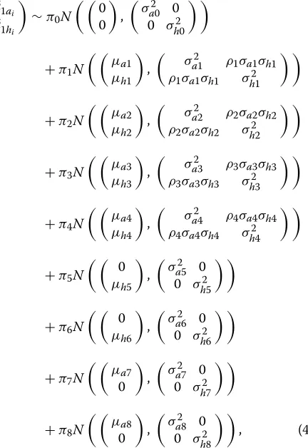
Tailoring the mixture model to two-species experiments with restrictions on the parameters made according to Table 1 and assuming that the treatment effects for non-differentially expressed genes are deterministically zero, i.e.,(β1ai,β1hi)
T =(0, 0)T, the following bivariate normal
mixture model is adopted as the prior distribution of the vector(β1ai,β1hi)
T:
β1ai β1hi
∼π0N μμa0
h0
,
η2
a0 ρ0ηa0ηh0 ρ0ηa0ηh0 ηh20
+π1N μμa1
h1
,
η2
a1 ρ1ηa1ηh1 ρ1ηa1ηh1 ηh21
+π2N μμa2
h2
,
η2
a2 ρ2ηa2ηh2 ρ2ηa2ηh2 ηh22
+π3N μμa3
h3
,
η2
a3 ρ3ηa3ηh3 ρ3ηa3ηh3 ηh23
+π4N μμa4
h4
,
η2
a4 ρ4ηa4ηh4 ρ4ηa4ηh4 ηh24
+π5N μμa5
h5
,
η2
a5 ρ5ηa5ηh5 ρ5ηa5ηh5 ηh25
+π6N μμa6
h6
,
η2
a6 ρ6ηa6ηh6 ρ6ηa6ηh6 ηh26
+π7N μμa7
h7
,
η2
a7 ρ7ηa7ηh7 ρ7ηa7ηh7 ηh27
+π8N μμa8
h8
,
η2
a8 ρ8ηa8ηh8 ρ8ηa8ηh8 ηh28
,
(3)
whereπkis the probability that an observation belongs to
thekth component, with8k=0πk =1 and πk≥0. The
following restriction of the parameter space is imposed: μa0 = 0, μh0 = 0, μa1 ≥ 0, μh1 ≥ 0, μa2 ≤ 0, μh2 ≤0,μa3 ≥0,μh3 ≤0,μa4 ≤0,μh4 ≥ 0,μa5 = 0, μh5 ≥ 0, μa6 = 0, μh6 ≤ 0, μa7 ≥ 0, μh7 = 0, μa8 ≤ 0,μh8 = 0,ηa0 = 0,ηh0 = 0,ηa5 = 0,ηa6 = 0, ηh7 = 0,ηh8 = 0,ρ0 = 0,ρ5 = 0,ρ6 = 0,ρ7 = 0, and ρ8=0.
According to the theory of least squares, the marginal distribution of(βˆ1ai,βˆ1hi)T, the parameter estimates, has means equal to the prior means of(β1ai,β1hi)T and vari-ances involving contributions from the prior distribu-tion of (β1ai,β1hi)T and the conditional distribution of
(βˆ1ai,βˆ1hi)T given(β1ai,β1hi)T. The marginal distribution of(βˆ1ai,βˆ1hi)Tis as follows:
ˆ
β1ai ˆ β1hi
∼π0N 00
,
σ2
a0 0
0 σh20
+π1N μμa1
h1
,
σ2
a1 ρ1σa1σh1 ρ1σa1σh1 σh21
+π2N μμa2
h2
,
σ2
a2 ρ2σa2σh2 ρ2σa2σh2 σh22
+π3N μμa3
h3
,
σ2
a3 ρ3σa3σh3 ρ3σa3σh3 σh23
+π4N μμa4
h4
,
σ2
a4 ρ4σa4σh4 ρ4σa4σh4 σh24
+π5N μ0
h5
,
σ2
a5 0
0 σh25
+π6N μ0
h6
,
σ2
a6 0
0 σh26
+π7N μ0a7
,
σ2
a7 0
0 σh27
+π8N μ0a8
,
σ2
a8 0
0 σh28 , (4)
An EM algorithm is developed to accomplish the nontriv-ial likelihood maximization, along with methodology for handling singular covariance matrices that arise during the implementation of the algorithm. (See the Appendix for details). Gene membership is determined according to the maximum posterior probability that an observa-tion(βˆ1ai,βˆ1hi)T comes from the kth component of the mixture.
Simulation
The following Monte Carlo simulation studies investi-gated the performance of the proposed mixture model using information across two species in comparison to the traditional microarray method using just one-species information when identifying genes associated with treat-ment stimulus under several different scenarios.
Several factors influence the sampling properties of the estimated treatment effects(βˆ1ai,βˆ1hi)Tusing the mixture model were considered in the simulation:
• Replicates (number of arrays) per treatment for each species:naandnhfor animals and humans,
respectively.
• Number of orthologous genes in each category:nk,
• Array noise:eaijandehijin (1) and (2). Also recall that, by assumption,eaijandehilare independent N(0,σa2)andN(0,σh2)random variables.
• Parameters in (3) by which the sampling distribution of(βˆ1ai,βˆ1hi)T is determined.
With so many variables, it is impractical to study the sampling properties of the fitted model without fixing some variables. That is, an experimental design for the simulation in which these factors are completely consid-ered is not feasible. The simulation study instead focused on three aspects. First, although high-density microarrays provide useful genome-wide data, they are often associ-ated with a substantial amount of experimental noise that could affect the performance of the analysis. Hence, it is of interest to investigate how the array noise would affect the model efficiency on gene identification across species. Second, the sample size of cross-species experiment is likely to be different, and may be one of the deciding fac-tors of the power associated with the modeling approach. In particular, the efficiency of gene identification, whether the proposed model gains power over one-species experi-ments through pooling information across species, should be examined carefully, especially when the sample size of the experiments is small.
Third, over-fitting may be of concern. The proposed mixture model is, by its nature, highly structured and data driven. If the data are not driven by all nine categories as the model suggests, will the mixture model fail? Is the pro-posed model flexible enough to handle different types of data structure? To examine the model performance sys-tematically and to test if the proposed model will fail when too many components are used to fit the data where there are actually fewer clusters, two types of data were gener-ated: all nine categories non-empty (case I) and some of the nine components empty (case II).
In simulation studies case I and case II, two methods of gene identification were implemented: the proposed mixture model, utilizing information across two different species, and the traditionaltstatistics adjusting for mul-tiple comparisons based on single-species data. Five hun-dred data sets were generated for each different scenario under each simulation study.
Parameter determination and data generation
Theoretically, the number of genes in category 0 (non-differentially expressed in both species) should dominate others, and every other category may comprise some genes. Orthology information from HomoloGene of the National Center for Biotechnology Information (NCBI) (http://www.ncbi.nlm.nih.gov/homologene) and Mouse Genome Informatics (MGI) of Jackson Laboratory [18] and the practical experience gained from analysis of two-species gene expression experiments at GlasoSmithKline
(GSK) was used as reference to determine a reasonable number of genes in each category.
The vectors of the number of genes in each cate-gory (n0,n1,. . .,n8)T determined for simulation stu-dies case I and case II are categories (6, 000, 30, 30, 30, 30, 100, 100, 100, 100)T and categories (6, 000, 30, 30, 0, 0, 100, 0, 100, 0)T, respectively. For experiments across species, sample sizes may differ. Considering that this proposed bivariate method could benefit from pooling information across species, especially when the sample size is small, and the practical situation, two sce-narios were implemented: the number of replicates per treatment for each species is equal and small, and the number of replicates per treatment for animals is greater than humans. In addition, to evaluate how robust the proposed method is against array noise, two situations were considered: the two experiments are equally noisy and the human data are noisier than the animal’s. Fur-thermore, values of parameters in (3) for the sampling distribution of (βˆ1ai,βˆ1hi)T were predetermined. Vari-ances of (β1ai,β1hi)
T in each component were assumed
to be the same:ηa21 = ηa22 = ηa23 = ηa24 = ηa27 = η2a8 = η2
h1 =η2h2= η2h3 =η2h4 =η2h5 =η2h6 =0.25. The corre-lation between (β1ai,β1hi)T in categories (1, 2, 3, 4) was assumed to be 0.9, i.e.,ρ1=ρ2=ρ3=ρ4=0.9. Nonzero component means(μak,μhk)T,k = 0,. . ., 8, were
deter-mined so that |μ/η| = 0.5 or 1.5. The combination of these parameters resulted in eight different scenarios for each case as presented in Table 2. Note that |μβ1ai|and |μβ1hi|represent the absolute value of the mean vector of (β1ai,β1hi)T.
After generating(β1ai,β1hi)T accordingly, the next step is to simulate the two species gene expression data Xa
andXhbased on linear models (1) and (2). Note thatβ0ai and β0hi are independent N(8, 1) random variables for differentially expressed genes and deterministically 0 for non-differentially expressed genes.
Simulation results
It is of interest to compare how effective the mixture model is on gene identification using information across two species with the conventional one-species approach. The conventional two-sample t test for gene selection was performed using just single species data (animals or humans) and a multiplicity adjustment was made according to the procedure proposed by Benjamini and Hochberg [19].
Table 2 Combination of parameters for simulation studies case I and case II
Case I sim1 sim2 sim3 sim4 sim5 sim6 sim7 sim8
na 10 10 10 10 100 100 100 100
nh 10 10 10 10 10 10 10 10
|μβ1ai| 0.25 0.75 0.25 0.75 0.25 0.75 0.25 0.75
|μβ1hi| 0.25 0.75 0.25 0.75 0.25 0.75 0.25 0.75
σ2
a 0.1 0.1 0.1 0.1 0.1 0.1 0.1 0.1 σ2
h 0.1 0.1 0.3 0.3 0.1 0.1 0.3 0.3
Case II sim9 sim10 sim11 sim12 sim13 sim14 sim15 sim16
each simulated data set, FDRIwas calculated as (number
of genes that are erroneously classified into categories (1, 2, 3, 4, 5, 6))/(total number of genes classified into categories (1, 2, 3, 4, 5, 6)). This was to ensure a fair com-parison between the mixture model and the conventional one-species method. FDRII was calculated in the same
fashion. Avg FDRI and Avg FDRII are simply the
aver-aged values of FDRIand FDRII across the 500 simulated
data sets. When the estimated nominal FDR = 0, i.e., the mixture model did not falsely categorize any genes, the nominal FDR for the single-species method was con-trolled at 0.0001. The second section of Table 3, categories (1, 2, 3, 4, 7, 8), represents the number of genes classified into categories (1, 2, 3, 4, 7, 8) using the mixture model (Mixture) and number of genes selected using animal data
alone (Animal only). Beneath each set of eight simulation cases is Tukey’s Honestly Significant Difference (HSD) for a familywise error rate of 0.05 for the results obtained using the proposed mixture model. Tukey’s HSD was calculated asq0.05(8, 3, 992)×(MS(Error)/500)1/2, since there were eight simulation cases (500 simulated data sets in each situation) in each simulation study (case I and case II) and the error degree of freedom was 3,992. MS(Error) denotes the error mean square (= Error sum of squares/Error degree of freedom, see Table 4). q0.05(8, 3, 992)=4.29.
The effect of array noise on the mixture model can be easily seen from the column of Avg FDRI and by
comparing the results of sim1 vs. sim3, sim5 vs. sim7, sim9 vs. sim11, and sim13 vs. sim15. These are the cases
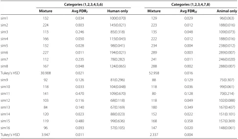
Table 3 The number of genes selected based on (a) bivariate mixture model, (b) conventional one-species approach
Categories (1,2,3,4,5,6) Categories (1,2,3,4,7,8)
Mixture AvgFDRI Human only Mixture AvgFDRII Animal only
sim1 132 0.034 100(0.070) 129 0.029 96(0.063)
sim2 224 0.003 145(0.021) 223 0.012 188(0.016)
sim3 113 0.246 85(0.318) 135 0.048 109(0.073)
sim4 166 0.050 115(0.043) 222 0.012 188(0.016)
sim5 132 0.028 98(0.041) 234 0.004 238(0.012)
sim6 227 0.011 194(0.021) 289 0.003 289(0.007)
sim7 112 0.235 78(0.282) 241 0.011 246(0.020)
sim8 167 0.048 124(0.065) 288 0.002 288(0.007)
Tukey’s HSD 30.908 0.021 52.958 0.016
sim9 92 0.126 81(0.296) 88 0.129 75(0.307)
sim10 118 0.033 104(0.048) 118 0.036 99(0.061)
sim11 141 0.470 109(0.670) 80 0.128 70(0.214)
sim12 103 0.116 68(0.118) 118 0.049 102(0.088)
sim13 84 0.140 67(0.169) 180 0.349 167(0.407)
sim14 120 0.023 88(0.023) 152 0.022 151(0.101)
sim15 119 0.480 99(0.636) 168 0.358 157(0.369)
sim16 96 0.093 57(0.105) 147 0.020 148(0.061)
Tukey’s HSD 3.947 0.011 2.337 0.004
Under simulation studies case I and case II. Numbers in parentheses are the observed FDRs. Averaged over the 500 simulated datasets. Tukey’s HSD for anαlevel of
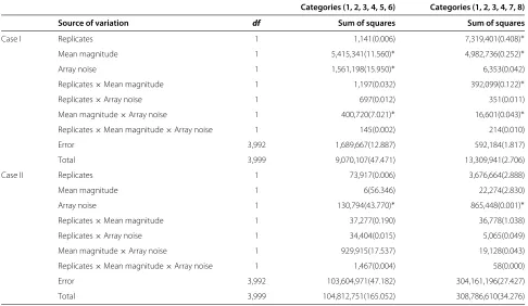
Table 4 ANOVA table to quantify variability
Categories (1, 2, 3, 4, 5, 6) Categories (1, 2, 3, 4, 7, 8)
Source of variation df Sum of squares Sum of squares
Case I Replicates 1 1,141(0.006) 7,319,401(0.408)∗
Mean magnitude 1 5,415,341(11.560)∗ 4,982,736(0.252)∗
Array noise 1 1,561,198(15.950)∗ 6,353(0.042)
Replicates×Mean magnitude 1 1,197(0.032) 392,099(0.122)∗
Replicates×Array noise 1 697(0.012) 351(0.011)
Mean magnitude×Array noise 1 400,720(7.021)∗ 16,601(0.043)∗
Replicates×Mean magnitude×Array noise 1 145(0.002) 214(0.010)
Error 3,992 1,689,667(12.887) 592,184(1.817)
Total 3,999 9,070,107(47.471) 13,309,941(2.706)
Case II Replicates 1 73,917(0.006) 3,676,664(2.888)
Mean magnitude 1 6(56.346) 22,274(2.830)
Array noise 1 130,794(43.770)∗ 865,448(0.001)∗
Replicates×Mean magnitude 1 37,277(0.190) 36,778(1.038)
Replicates×Array noise 1 34,404(0.015) 5,065(0.049)
Mean magnitude×Array noise 1 929,915(17.537) 19,128(0.043)
Replicates×Mean magnitude×Array noise 1 1,467(0.004) 58(0.000)
Error 3,992 103,604,971(47.182) 304,161,196(27.427)
Total 3,999 104,812,751(165.052) 308,786,610(34.276)
ANOVA was performed independently for simulation studies case I and case II to quantify the variability among the results (gene counts and observed FDRs). Numbers
in parentheses are the sum of squares for the observed FDRs. For gene counts, *indicates which sources of variability could be declared significant at levelα=0.05.
with smaller means and variances for humans which change from 0.1 to 0.3 for each pair of comparisons. The differences between the observed FDRs for these four groups were at least 0.2 and 0.3 for case I and case II, respectively. In contrast, when means were larger, changes of variances did not seem to affect the results in the sense that the corresponding observed FDRs had barely changed while the variances of human increased. The observed FDRs for animals were not as sensitive to the array noise on humans as the observed FDRs for humans.
Under both simulation studies case I and case II, increasing the number of replicates in the animal exper-iment helped the gene identification for animals: more animal genes were identified for sim5 to sim8 than for sim1 to sim4, and for sim13 to sim16 than for sim9 to sim12. The corresponding FDRs were also lower for sim5 to sim8 and sim13 to sim16. In contrast, increasing the number of replicates in the animal experiment did not significantly improve the results of gene identification for humans.
Table 4 is the summary of a three-way analy-sis of variance (ANOVA). Three factors, each with two levels, were used in the analysis: replicates ((na,nh)T = (10, 10)T or (100, 10)T), mean
magni-tude ((|μβ1ai|,|μβ1hi|)T = (0.25, 0.25)T or (0.75, 0.75)T),
and array noise ((σa2,σh2)T = (0.1, 0.1)T or (0.1, 0.3)T). This analysis, performed independently, quanti-fies the variability among the results (gene counts and observed FDRs) obtained using the proposed mixture model in Table 3 for the 16 different simu-lated situations under simulation studies case I and case II.
Throughout the 16 simulation cases, with nominal FDR controlled at FDRI, the bivariate mixture model
outper-formed the single-species method for human gene iden-tification by always recognizing more genes with lower observed FDRs. For the animal part, the mixture model performed at least as well as the single-species method on gene selection by identifying at least as many genes. Notice that selecting genes related to humans (categories (1, 2, 3, 4, 5, 6)) seemed to be associated with higher false discovery rate than selecting genes related to animals (cat-egories (1, 2, 3, 4, 7, 8)). Furthermore, the observed FDRs were lower for case I than for case II, regardless of the type of genes interested (differentially expressed for humans or animals).
Application: the mouse and human type II diabetes experiment
Background introduction
A systems biology study was completed by GlaxoSmithKline (GSK) to study the efficacy of type II diabetes drugs in both preclinical (mice) and clinical (humans) experi-ments. The mouse and human data were collected and preprocessed using Affymetrix MAS 5.0 at the probe set level on Affymetrix MOE430A array and Human Genome U133 Plus 2.0 array, respectively. For mice, the total num-ber of probe sets was 22,690. Mice were fed a diet enriched in fat (58% kcal from fat) for 8 weeks prior to treatment. Most of the mice of this susceptible strain developed obesity and mild hyperglycemia and hyperinsulinemia. Control mice on an 11% low fat diet remained normal. The mouse treatment arm consisted of a diabetes drug at multiple dose levels with vehicle controls over a 2-week period. The study was a full factorial design, where 40 ani-mals in high fat diet and 40 aniani-mals in low fat diet were randomized to receive either placebo, or different dosages of the type II diabetes drug (low, medium or high). Note that the results for mice were measured at one time point, the end of the study. For simplicity, only integration results on animals treated with placebo (10 mice) or high dose of the drug (9 mice) were demonstrated.
On the other hand, there were 54,676 probe sets in the human data set and all 59 subjects were type II diabetes patients. The gene expression measurements for human subjects were collected twice during the experiment, one at baseline before the treatment started (week 0) and the other one at the completion of the study (week 8). Among the 59 subjects, 14 only had data for only one time point and hence were not included in further data analysis. Sub-jects in the clinical trial were treated by either placebo, or three other type II diabetes drugs, including the one given to the mice. Titrated dosing was implemented to ensure that each person received his/her dose based on his/her body profile. Human subjects treated with placebo (num-ber of subjects=11) and the same type II diabetes drug given to mice (number of subjects=13) were used in this analysis. Besides being measured at two time points, other information contained in the human data and used in the data analysis included: prior therapy (four categorical lev-els) and concomitant medication status (two categorical levels).
Data for both species were logarithmic transformed (base equal to 2). Methods for combining information from multiple probe sets that were not identical have been discussed in many publications [20,21]. A gene-level tran-script value in order to pair the mouse and human genes through orthology was obtained by averaging probe sets across a gene. This resulted in 13,483 and 20,252 genes for mouse and human, respectively. Missing values were replaced with array means in both data sets.
The mouse and human orthology information, MGI release 4.32, was used to map the mouse and human orthologous genes. Human and mouse orthologs (17,834) were included in release 4.32. Combining the information among MGI release 4.32 and mouse and human genes from the GSK data gave a total of 11,922 orthologs.
In addition to the measurements of gene expression for both mice and humans, different efficacy endpoints, such as blood glucose, insulin, hemoglobin A1c (HbA1c), and others were also measured during the preclinical and clin-ical experiments by GSK in order to evaluate the effect of treatment intervention on both species.
The purpose of this data analysis was to evaluate the capability of the proposed mixture model, an approach utilizing the information across two species, to identify genes that may help scientists reveal the biological simi-larity between two species (ex: mouse and human), essen-tially genes in categories(1, 2, 3, 4), and so to improve the efficiency of drug development by decreasing the com-pound attrition rate from preclinical trials to clinical trials.
Data analysis
The estimated treatment effects for mice and humans are obtained by the following independent simple linear models:
Xaij=β0ai+β1aiTaj+eaij, (5)
Xhweek8
il =β0hi+X
week0
hil +β1hiThl+β2hiPriorTherapy +β3hiConMed+ehil, (6)
where i = 1,. . ., 11, 922 (number of orthologs); j = 1,. . ., 19 (number of mice); l = 1,. . ., 24 (number of humans). Xaij, Xhweekil 0 and X
week8
hil are gene expressions from the ith orthologous gene for the jth mouse, gene expression from the ith orthologous gene for the lth human before treatment intervention, and gene expres-sion from theith orthologous gene for the lth human at the completion of the clinical experiment, respectively. Taj andThl are {0, 1} treatment indicators, and eaij and ehil are independentN(0,σ2
a)andN(0,σh2)random
vari-ables. Additionally, there are two more covariates in the human model: PriorTherapy (a four-level categorical vari-able indicating patients’ therapy prior to the clinical trial) and ConMed (a two-level categorical variable for con-comitant medication status).
better understand the mechanism of drug activities in clinical trials.
Results
Parameter estimation
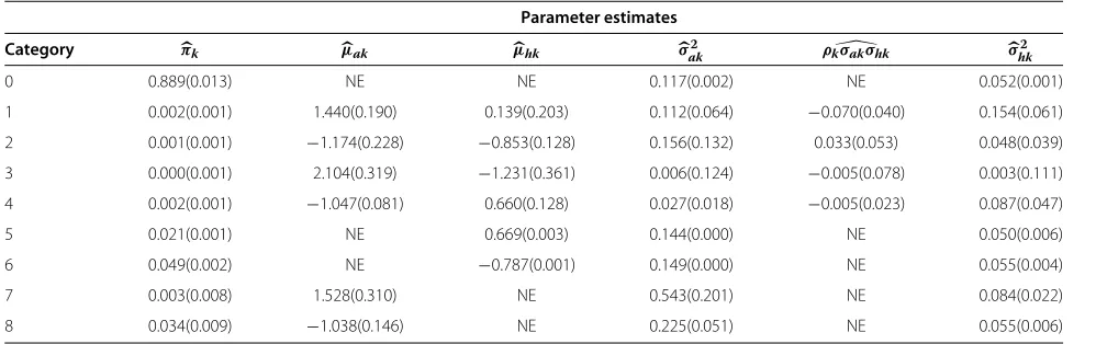
The maximum likelihood estimates of the parameters in the bivariate normal mixture model using the EM algo-rithm are given in Table 5. The estimated mixture weight for category 0 wasπ0 = 0.889 indicating approximately 10,599 (11, 922 × 0.889) pairs of uninteresting mouse and human orthologs. (μa,μh)T denotes the mean
vec-tor of each mixture component. The estimated treatment effect means of mice were in general larger than that of humans, indicating that the magnitude of the difference of expression in genes due to treatment intervention in mice tended to be larger than in genes where differential expression is exhibited in humans. The estimated variance for miceσak2 tended to be larger than that for humansσhk2, suggesting that overall, the variability in the mouse data set was larger than the human data set. The estimated correlation coefficients between the treatment effects for both species were(−0.531, 0.380,−1, 0.102)for categories (1, 2, 3, 4), respectively. The estimated correlation for cat-egory 3 was based on only two observations. Standard errors of the parameter estimates from the two-species experiment were obtained by bootstrapping with 1,000 bootstrap replicates. Based on the bootstrap standard errors, there was little evidence of bias for the parameter estimates.
Gene identification
The vector of the number of genes identified for each category was (nˆ0,nˆ1,. . .,nˆ8)T = (10,814, 41, 12, 2, 20, 168, 578, 12, 275)T. Figure 1 displays the scatter plots of
(βˆ1ai,βˆ1hi)
T before and after gene membership
identifi-cation, including the scatter plot of (βˆ1ai,βˆ1hi)
T for all
orthologs, orthologs after eliminating the uninteresting
ones (orthologs not in category 0), and orthologs reacting to the treatment stimulus for both species (orthologs in categories (1, 2, 3, 4)).
Based on the bivariate mixture model, among the 11,922 pairs of orthologs, 10,814 pairs did not react to the drug treatment for either species, 75 pairs of orthologs (sum of the gene counts in categories 1 through 4) showed evidence of differentiation between treatments for both species. Genes in categories (5, 6, 7, 8) are also poten-tial candidates for further investigation to improve the process of drug development since studying these genes might uncover the myth of the overall high attrition rate of a drug compound from preclinical trials to clinical trials.
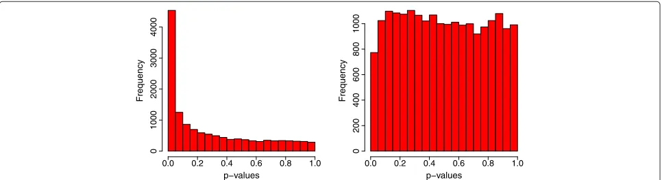
In comparison, an attempt was made to identify differ-entially expressed human genes using solely the human data, i.e., traditionaltstatistics were used to test whether or not β1hi = 0 and the approach of Benjamini and Hochberg [19] was used to adjust for multiple compar-isons. With the nominal FDR controlled at 0.01, 0.1, 0.5, and 0.9, this single-species method failed to identify any differentially expressed human genes at any levels of FDR. With the p values histograms in Figure 2 showing an obvious difference between the observed significance of differential expression for mice and humans, specifically, thepvalues were nearly uniformly distributed for humans, the result was not surprising.
Concluding remarks
This research was motivated by a fundamental yet still not well-understood problem in the drug development process. The results obtained in preclinical animal trials do not seem to translate well enough to make inferences for human clinical trials, resulting in an undesirably high attrition rate in human experiments. A bivariate mixture model which utilizes information across two species was proposed to identify genes that exhibit similar patterns of expression across species, with the hope that studying
Table 5 Parameter estimates of the bivariate mixture model
Parameter estimates
Category πk μak μhk σak2 ρkσakσhk σhk2
0 0.889(0.013) NE NE 0.117(0.002) NE 0.052(0.001)
1 0.002(0.001) 1.440(0.190) 0.139(0.203) 0.112(0.064) −0.070(0.040) 0.154(0.061)
2 0.001(0.001) −1.174(0.228) −0.853(0.128) 0.156(0.132) 0.033(0.053) 0.048(0.039)
3 0.000(0.001) 2.104(0.319) −1.231(0.361) 0.006(0.124) −0.005(0.078) 0.003(0.111)
4 0.002(0.001) −1.047(0.081) 0.660(0.128) 0.027(0.018) −0.005(0.023) 0.087(0.047)
5 0.021(0.001) NE 0.669(0.003) 0.144(0.000) NE 0.050(0.006)
6 0.049(0.002) NE −0.787(0.001) 0.149(0.000) NE 0.055(0.004)
7 0.003(0.008) 1.528(0.310) NE 0.543(0.201) NE 0.084(0.022)
8 0.034(0.009) −1.038(0.146) NE 0.225(0.051) NE 0.055(0.006)
Figure 1Scatter plots of the estimated treatment effects(βˆ1ai,βˆ1hi)Tbefore and after gene membership identification.From left to right:
all orthologs, orthologs differentially expressed in either species (categories(1, 2, 3, 4, 5, 6, 7, 8)), and orthologs differentially expressed in both species (categories(1, 2, 3, 4)).
genes could help understand biological differences across species at the molecular level and ultimately help reduce attrition in drug development. It is also of great interest to identify genes active in animal, but not in human since studying this group of genes might lead to answers that explain why some drug trials fail in translation to humans. The comprehensive simulation study suggested that the proposed model, though highly structured, can accommo-date various configurations of differential gene expression, especially when the magnitude of differential expression due to different treatment intervention was weak.
In the application of the bivariate mixture model on the GSK type II diabetes experiment, the mixture model was able to separate differentially expressed genes from non-differentially expressed genes. A potential multi-gene predictor may be developed according to the genes iden-tified by the bivariate mixture model to benefit patients in therapeutic decision making.
The mixture model is highly structured, with strong but somewhat simplifying assumptions. The grouping of all genes for which the expression difference is positive in both species into a single category parameterized by
a single bivariate mean may be somewhat of a simplistic approach. In practice, the data may not be normally dis-tributed or be comprised by exactly nine groups and lead to bias and inefficiency. Forcing the normality assump-tion and the grouping may be inefficient. However, by modeling the least squares estimates of the expression differences as bivariate realizations from a distribution with a single mean vector, some flexibility in the model is retained. It is perhaps less important to precisely quantify the magnitude of the expression difference than to deter-mine whether it is positive or negative and whether or not the direction is preserved across species.
Using the proposed mixture model for gene identifi-cation is completely data-driven. The simulation study in Section ‘Simulation’ indicated that the mixture model at times report a poor observed false discovery rate due to large variability in measurement of expression. Cur-rently, gene membership classification is determined by maximizing the posterior probability that observationyi
belongs to thekth cluster. It is possible to choose costs to attach weight to different types of misclassification and then choose a classification rule to minimize expected
0.0 0.2 0.4 0.6 0.8 1.0
0
1000
2000
3000
4000
p−values
Frequency
0.0 0.2 0.4 0.6 0.8 1.0
0
200
400
600
800
1000
p−values
Frequency
cost. This rule may lead to a more desirable list that can better accommodate goals for future research.
The mixture model currently only handles data with two treatments/cancer types/drugs, i.e., data containing only two-level variables. In practice, it is often the case that an experiment is run under multiple conditions. An exten-sion of the model to handle experiments with factors with three-or-more levels is an important future work.
This approach focuses on identifying orthologs that show same/opposite mechanism between two species. However, genes identified by the bivariate mixture model (genes in categories (1, 2, 3, 4)) may not lead to the most powerful model for prediction of cancer types/response status for either one of the species. The most power-ful model may be based on those human genes that lie in categories 5 and 6. For those genes, the cor-responding animal genes show no signs of differential expression. Hence, incorporating prediction ability into the model or developing a prediction model that can help utilize the genes selected by the mixture model is of great interest and is an obvious candidate for future research.
Appendix
Mixture models and the EM algorithm
Estimating the parameters in (4) is nontrivial. Redner and Walker [22] offer an excellent review of estimating the parameters which determine a mixture density. In partic-ular, the paper is devoted to a particular iterative proce-dure for numerically approximating maximum likelihood estimates (MLE) of the parameters in mixture densities. This method was formalized by Dempster et al. [23] and termed the EM (Expectation-Maximization) algorithm, and is used for numerically approximating the maximum likelihood estimates for (4).
The EM algorithm with no constraints
For a finite mixture model withCcomponents, given data
y with independent multivariate observationsy1,. . .,yg, eachyiis taken to be a realization of the mixture probabil-ity densprobabil-ity function,
f(yi|)= C
k=1
πkfk(yi|θk),
where = (θ1,. . .,θC,π1,. . .,πC)T, a vector of
un-known parameters.fk andθk are the density and
param-eters of the kth component in the mixture, respectively. πk is the probability that an observation arises from the
kth component. Note that πk ≥ 0 and
C
k=1πk =
1. For classification purpose and to achieve minimum misclassification rates, yi is assigned to the population (category) for which the posterior probability that yi
belongs to the kth cluster (the kth component of the
mixture) is maximized. The posterior probability is given by
τk(yi;)=
πkfk(yi|θk)
C
h=1πhfh(yi|θh)
.
In summary, the EM algorithm may be implemented to maximize the likelihood of a multivariate normal mixture model by following these two steps:
E-step: The E-step on the ( j+1) iteration takes the con-ditional expectation of the complete-data log likelihood, given the observed data(Q(|(j))).
At the(j+1)iteration, the E-step results in
Q(|(j))=
g
i=1
C
k=1
τk(yi;(j))(logπk+logfk(yi|θk)),
(7)
where fk(yi|θk) = (2π)−
p
2|k|−12e−12(yi−μk)T−k1(yi−μk)
andτk(yi;(j))=
π(j)
k fk(yi|θ( j)
k )
C
h=1π(
j)
h fh(yi|θ( j)
h )
.
M-step: The M-step on the ( j+1) iteration requires the
global maximization of Q(|(j))with respect to over the parameter space to give the updated estimate(j+1).
ˆ π(j+1)
k =
g
i=1τk(yi;(j))
g ; (8)
ˆ μ(j+1)
k =
g
i=1τk(yi;(j))yi
g
i=1τk(yi;(j))
; (9)
(kj+1)=
g
i=1τk(yi;(j))(yi−μk)T(yi−μk)
g
i=1τk(yi;(j))
. (10)
The iterations of the EM algorithm continue until some stopping criterion is met, such as the difference of the con-ditional expectation of the complete-data log likelihood at the(j+1)step and the conditional expectation of the complete-data log likelihood at the jstep is sufficiently small, i.e.,
Q( (j+1)| (j))−Q( (j)| (j))≤ .
Throughout this research, =0.0001.
The EM Algorithm with constraints
that (4) is a bivariate normal mixture with nine compo-nents and the density for each component can be written as
fk
yi|θk
=e −1
2σ2 1
akσhk2(1−ρ2k)
σ2
hk yai−μak
2
−2ρkσakσhk yai−μak yhi−μhk+σ2
ak yhi−μhk
2
2πσ2 akσ
2 hk
1−ρ2 k
,
whereyi =(yai,yhi)
T =(βˆ
1ai,βˆ1hi)
T andθ
k =(μak,μhk, σ2
ak,σ 2
hk,ρk)
T.
The solution for the E-step remains the same. The membership probability τk(yi;(j)) can be obtained by
taking the conditional expectation of the complete-data log likelihood, given the observed data.
As for the M-step, the MLE forπk remains the same,
ˆ π(j+1)
k =
g
i=1τk(yi;(j))
g . However, the MLEs forμk and k need to be modified according to the constrained
parameter space for each mixture component.
Essentially, the MLEs on the (j + 1) iteration for (μak,μhk)T,k=1,. . ., 4, are
ˆ μ(j+1)
a1 =
⎧ ⎨ ⎩
g
i=1τ1(yi;(j))yai g
i=1τ1(yi;(j))
ifgi=1τ1(yi;(j))yai≥0;
0 otherwise.
ˆ μ(j+1)
h1 =
⎧ ⎨ ⎩
g
i=1τ1(yi;(j))yhi g
i=1τ1(yi;(j))
ifgi=1τ1(yi;(j))yhi≥0;
0 otherwise.
ˆ μ(aj2+1) =
⎧ ⎨ ⎩
g
i=1τ2(yi;(j))yai g
i=1τ2(yi;(j)) if
g
i=1τ2(yi;(j))yai≤0;
0 otherwise.
ˆ μ(j+1)
h2 =
⎧ ⎨ ⎩
g
i=1τ2(yi;(j))yhi g
i=1τ2(yi;(j))
ifgi=1τ2(yi;(j))yhi≤0;
0 otherwise.
ˆ μ(j+1)
a3 =
⎧ ⎨ ⎩
g
i=1τ3(yi;(j))yai g
i=1τ3(yi;(j))
ifgi=1τ3(yi;(j))yai≥0;
0 otherwise.
ˆ μ(hj3+1) =
⎧ ⎨ ⎩
g
i=1τ3(yi;(j))yhi g
i=1τ3(yi;(j))
ifgi=1τ3(yi;(j))yhi≤0;
0 otherwise.
ˆ μ(j+1)
a4 =
⎧ ⎨ ⎩
g
i=1τ4(yi;(j))yai g
i=1τ4(yi;(j))
ifgi=1τ4(yi;(j))yai≤0;
0 otherwise.
ˆ μ(j+1)
h4 =
⎧ ⎨ ⎩
g
i=1τ4(yi;(j))yhi g
i=1τ4(yi;(j))
ifgi=1τ4(yi;(j))yhi≥0;
0 otherwise.
The MLEs ofk, k = 1,. . ., 4, at the(j+1) M-step
remain unchanged as in (10).
The MLEs on the(j+1)iteration for(μak,μhk)T,k=
5,. . ., 8, are
ˆ μ(j+1)
h5 =
⎧ ⎨ ⎩
g
i=1τ5(yi;(j))yhi g
i=1τ5(yi;(j))
ifgi=1τ5(yi;(j))yhi≥0;
0 otherwise.
ˆ μ(hj6+1) =
⎧ ⎪ ⎪ ⎨ ⎪ ⎪ ⎩ g
i=1τ6(yi;(j))yhi g
i=1τ6(yi;(j))
ifgi=1τ6(yi;(j))yhi≤0;
0 otherwise.
ˆ μ(j+1)
a7 =
⎧ ⎨ ⎩
g
i=1τ7(yi;(j))yai g
i=1τ7(yi;(j))
ifgi=1τ7(yi;(j))yai≥0;
0 otherwise.
ˆ μ(j+1)
a8 =
⎧ ⎨ ⎩
g
i=1τ8(yi;(j))yai g
i=1τ8(yi;(j))
ifgi=1τ8(yi;(j))yai≤0;
0 otherwise.
The MLE fork,k=0, 5, 6, 7, 8, on the(j+1)iteration is
k= ⎛ ⎜ ⎝ g
i=1τk(yi;(j))y2ai g
i=1τk(yi;(j))
0
0
g
i=1τk(yi;(j))y2hi g
i=1τk(yi;(j)) ⎞ ⎟ ⎠.
Regularized covariance matrices in the EM algorithm
this research. In Sato and Ishii [32], the regularized covari-ance matrix for thekth mixture component in the(j+1) M-step is
(j+1)
Rk =
(j+1)
k +α
tr((kj+1))
p Ip, (11)
where 0 ≤ α ≤ 1 is a small constant and Ip is a
p-dimensional identity matrix. If (kj+1) equals 0, then tr((kj+1))is set to be a small threshold value (0.0001 in this research).
Competing interests
The authors declare that they have no competing interests.
Authors’ contributions
YS, LZ, AM and JO have participated in the development of the proposed model. YS has drafted the manuscript. All authors read and approved the final manuscript.
Acknowledgements
The authors thank GlaxoSmithKline for sponsoring the systems biology study and collaborating in the data analyses.
Author details
1Dr. Su’s Statistics & Department of Human Nutrition, Food, and Animal Sciences, University of Hawaii at Manoa, Honolulu, HI 96822, USA.2Biomarker and Predictive Analytics, GlaxoSmithKline, 5 Moore Drive, Research Triangle Park, NC 27709, USA.3Department of Statistics, North Carolina State University, Raleigh, NC 27695, USA.
Received: 8 December 2011 Accepted: 23 June 2014 Published: 1 August 2014
References
1. FDA:Innovation and stagnation: challenge and opportunity on the critical path to new medical products.FDA White Paper2004. 2. Bolten B, DeGregorio T:Trends in development cycles.Nat Rev Drug
Discov2002,1:335–336.
3. Kola I:Landis J: Can the pharmaceutical industry reduce attrition rates?Nat Rev Drug Discov2004,3:711–715.
4. Braxton S, Bedilion T:The integration of microarray information in the drug development process.Curr Opin Biotechnol1998,9:643–649. 5. Debouck C, Goodfellow P:DNA microarrays in drug discovery and
development.Nat Genet1999,21:48–50.
6. Koonin E:An apology for orthologs - or brave new memes.Genome Biol2001,2(4):1005.1–1005.2.
7. Sonnhammer E, Koonin E:Orthology, paralogy and proposed classification for paralog subtypes.Trends Genet2002,18:619–620. 8. Theiben G:Secret life of genes.Nature2002,415:741.
9. Holbrook J, Sanseau P:Drug discovery and computational evolutionary analysis.Drug Discov Today2007,12:826–832. 10. Grigoryev D, Ma S, Irizarry R, Ye S, Quackenbush J, Garcia J:Orthologous
gene-expression profiling in multi-species models: search for candidate genes.Genome Biol2004,5:R34.1–R34.13.
11. Batzoglou S, Pachter L, Mesirov J, Berger B, Lander E:Human and mouse gene structure: comparative analysis and application to exon prediction.Genome Res2008,10:950–958.
12. Taher L, Rinner O, Garg S, Sczyrba A, Morgenstern B:AGenDA: gene prediction by cross-species sequence comparison.Nucleic Acids Res 2004,1:W305–W308.
13. Ogorek B:Orthology-based multilevel modeling of differentially expressed mouse and human gene pairs.PhD thesis2008.
14. Lelandais G, Vincens P, Badel-Chagnon A, Vialette S, Jacq C, Hazout S: Comparing gene expression networks in a multi-dimensional space to extract similarities and differences between organisms. Bioinformatics2006,22:1359–1366.
15. Park D, Park J, Park S, Park T, Choi S:Analysis of human disease genes in the context of gene essentiality.Genomics2008,92:414–418. 16. McLachlan G, Basford K:Mixture Models: Inference and Applications to
Clustering. New York: Marcel Dekker, Inc.; 1988.
17. McLachlan G, Peel D:Finite Mixture Models. New York: Wiley; 2000. 18. Blake J, Richardson J, Bult C, Kadin J:Eppig J, the Mouse Genome
Database Group: The Mouse Genome Database (MGD): the model organism database for the laboratory mouse.Nucleic Acids Res2002, 30:113–115.
19. Benjamini Y, Hochberg Y:Controlling the false discovery rate: a practical and powerful approach to multiple testing.J Roy Stat Soc B 1995,57:289–300.
20. Li C, Wong W:Model-based analysis of oligonucleotide arrays: expression index computation and outlier detection.Proc Natl Acad Sci USA2001,98:31–36.
21. Li C, Zhu D, Cook M:A statistical framework for consolidating sibling probe sets for Affymetrix GeneChip data.BMC Genomics2008,9:188. 22. Redner R, Walker H:Mixture densities, maximum likelihood and the
EM algorithm.J Soc Ind Appl Math1984,26(2):195–239.
23. Dempster A, Laird N, Rubin D:Maximum likelihood from incomplete data via the EM algorithm.J Roy Stat Soc B1977,39:1–38.
24. Fraley C, Raftery A:How many clusters? Which cluster method? Answer via model-based cluster analysis.Comput J1998, 41(8):578–588.
25. Fraley C, Raftery A:Model-based clustering, discriminant analysis, and density estimation.J Am Stat Assoc2002,97(458):611–631.
26. Robotka Z, Zempleni A, Hajas C, Seres C, Balazs S:Genetic algorithms and grid technologies in clustering, an example: clustering of images.Qual Reliab Eng Int2008,24:693–703.
27. Vlassis N, Likas A:A greedy EM algorithm for Gaussian mixture.Neural Process Lett2002,15:77–87.
28. Hsieh P, Landgrebe D:Statistics enhancement in hyperspectral data analysis using spectral-spatial labeling, the EM algorithm, and the leave-one-out covariance estimator.InSPIE International Symposium on Optical Science, Engineering, and Instrumentation. Denver, Colorado; 1999:19–24.
29. Snoussi H, Mohammad-Djafari A:Penalized maximum likelihood for multivariate Gaussian mixture.InAIP Conference Proceedings; 2002:36–46.
30. Mao J, Jain A:A self-organizing network for hyperellipsoidal clustering (HEC).IEEE Trans Neural Netw1996,7:16–29.
31. Archambeau C, Verleysen M:Fully nonparametric probability density function estimation with finite gaussian mixture models.InFifth International Conference on Advances in Pattern Recognition. 10-13 Dec 2003. Calcultta, India; 2003:81–84.
32. Sato M, Ishii S:On-line EM algorithm for the normalized Gaussian network.Neural Comput2000,12:407–432.
33. Lee K:A new, EM algorithm for resource allocation network.In Pattern Recognition and Data Mining. Berlin: Springer; 2005.
doi:10.1186/1479-7364-8-12
Cite this article as:Suet al.:Mixture models for gene expression