Functional Circular Relationship Models
ALi Hassan Abuzaid
Department of Mathematics, Faculty of Science Al-Azhar University-Gaza, Gaza, Palestine [email protected]
Abstract
If the interest is to calibrate two instruments then the functional relationship models are more appropriate than regression models. Fitting a straight line when both variables are circular and subject to errors has not received much attention.
In this paper, we consider the problem of detecting influential points in two functional relationship models for circular variables. The first is developed based on the simple circular regression model, demoted by (SC), while the second is derived from the complex linear regression model and denoted by (CL). The covariance matrices are derived and then the COVRATIO statistics are formulated for both models. The cut-off points are obtained and the power of performance is examined via simulation studies.
The performance of COVRATIO statistics depends on the concentration of error, sample size and level of contamination. In the case of the linear relationship between two circular variables, COVRATIO statistics of the (SC) model performs better than the (CL).
Furthermore, a novel diagram, the so-called spoke plot, is utilized to detect possible influential points. For illustration purposes, the proposed procedures are applied on real data of wind directions measured by two different instruments. COVRATIO statistic and the spoke plot were able to identify two observations as influential points.
Keywords: Correlation, Radar, Errors, Estimation, Wind.
1. Introduction
In practice, calibrating two or more instruments producing angular measurements can be statistically handled via circular functional relationship models (see Caires and Wyatt, 2003, Hassan, et al, 2010). Taking into the account that the compared variables are subjected to errors. Thus, the existence of one or more influential points in a data set is more likely to affect the efficiency of a suggested model.
Up to date, there are only two published papers consider the problem of influential points in the circular functional relationship models. The first studies the linear functional relationship model for circular variables (SC) which proposed by Caires and Wyatt (2003), and the COVRATIO statistic is derived to detect possible influential points by Hussin, et al. (2010). The second paper treats the circular variables as complex numbers and then the complex linear functional relationship model (CL) was developed and the
Thus, introducing the slope parameter into the model will make the covariance matrix more informative.
On the other hand, the investigation of COVRATIO statistic performance for the (CL) model is questionable, where the real and imaginary components were contaminated separately, and as given by Hussin and Abuzaid (2012) the power of COVRATIO statistic was more than 0.15 for free contamination case.
In this paper, we will compare the performances of the COVRATIO statistics in detecting the influential points in the (SC) and the (CL) models by considering two issues: the first is to introduce the slope parameter for the (SC) model, and the second is to contaminate both model consistently.
The rest of the paper is organized as follows: the following section presents the considered two functional relationship models of circular data. Section 3 discusses the derivation of the COVRATIO statistics, calculation of the cut-off points and the power of performance. A real data set is presented and analyzed in Section 4.
2. Functional Relationship Models of Circular Variables
Fitting a straight line when both variables are circular and subject to errors has not received much attention. In the following two subsections we consider two functional relationship models for circular variables and derive their corresponding COVRATIO
statistics.
2.1 Linear Functional Relationship Model for Circular Variables (SC)
For any two circular random variables X and Y measured with errors, Caires and Wyatt (2003) proposed the following model:
, ..., 1, = for ), 2 ( =
where , =
and
= X y Y Y X mod i n
xi i i i i i i i (1)
where i andi are independently distributed with von Mises distributions, that is
) (0,
i ~VM and i ~VM(0,). Under the same assumptions, Hussin (2008) extended model (1) to the (SC) model and it is given by:
, ..., 1, = for ), 2 ( =
where , =
and
= X y Y Y X mod i n
xi i i i i i i i (2)
where is the slope parameter. There are (n+4) parameters to be estimated, i.e.,
, , , and the incidental parameters X1,...,Xn. The MLE of the intercept parameter
is given by:
, 0 , 0 2
) / ( tan
, 0 )
/ ( tan
, 0 , 0 )
/ ( tan =
ˆ
1 1
1
C S C
S
C C
S
C S C S
where S
sin(yi ˆxi) and C
cos(yi ˆxi). The slope and Xi estimates aregiven by ,
) ˆ ˆ ˆ ( cos ˆ ) ˆ ˆ ˆ ( sin ˆ ˆ ˆ 0 0 0
1
i i i i i i X y X X y X and , ) ˆ ˆ ˆ ( cos ˆ ) ˆ ( cos ) ˆ ˆ ˆ ( sin ˆ ) ˆ ( sin ˆ ˆ 0 2 0 0 0 0 1 i i i i i i i i i i X y X x X y X x X X
where ˆ1 and Xˆi1 are improvements
of ˆ0 and Xˆi0, respectively, and .
Then we can find an estimate of for any value of from the equation
cos( ˆ ) cos( ˆ ˆˆ )
, 1= ) ( )
( xi Xi yi Xi
n A
A
For the case =1, the estimate of concentration parameter, ˆ may be obtained by using the approximation given in Fisher (1993):
, . 0.85 ) 3 4 ( 0.85 < 0.53 1 0.43 1.39 0.4 , 0.53 < 833 . 0 2 = 1 2 3 1 5 3 1 w w w w w w w w w w w w AHence, ˆ = A1(w) where { cos( ˆ ) cos( ˆ ˆˆ )}. 2
1
= xi Xi yi Xi
n
w
The second partial derivatives of the loglikelihood function with respect to the parameters are obtained and then the Fisher's information matrix is formulated to find the covariance matrix via finding its inverse. Then the following results can be obtained: (For detailed derivation see Hussin, 2008).
0 ) ˆ , ˆ cov( ) ˆ , ˆ
cov( ,
] ) ( )[ ˆ ( ˆ ) ˆ 1 ( ) ˆ
var( 2 2
2 2 i i i X X n A X , ] ) ( )[ ˆ ( ˆ ) ˆ 1 ( ) ˆ
var( 2 2
2 i i X X n A n , )] ˆ ( ) ˆ ( ˆ ˆ [ ˆ ) ˆ var( 2 A A
n
, and
] ) ( )[ ˆ ( ˆ ) ˆ 1 ( ) ˆ , ˆ
cov( 2 2
2 i i i X X n A X .
2.2 Complex Linear Functional Relationship Model for Circular variables (CL):
For any two circular random variables X and Y Hussin and Abuzaid (2012) proposed the complex linear functional relationship model, and it is given by:
j j j
j
j i x X i X
x sin )(cos sin )
(cos , and
j j j
j
j i y Y i Y
y sin )(cos sin )
(cos ,
where (cosY isinY )(cosX isin X ), for j=1,...,n,
where j and j are independently distributed errors from the bivariate complex
Gaussian distributions. The MLE of model parameters are given by:
, ) ˆ cos ˆ (cos 1
ˆ yj Xj
n , ) ˆ cos ˆ ˆ sin sin ˆ cos (cos 1 ˆ j j j j
j X y X X
y n and ˆ ˆ cos ˆ cos sin ˆ sin tan ˆ 1 j j j j j y x y x
X where 22 12 and
). ˆ sin sin ˆ cos (cos ˆ 2 )) cos ˆ cos ˆ ( ˆ 2 ˆ ˆ 1 ( 1 ) ˆ sin sin 2 ˆ cos cos 2 2 (
1 2 2
2 1 j j j j j j j j j j X y X y n y X n X x X x n
Due to the absence of the closed-form for ˆ,ˆ,Xˆjand ˆ12 the estimates may be obtained
iteratively. The asymptotic properties of ˆ andˆ are obtained from Fisher’s information matrix and given by:
, ) ( ) )( ( ) ˆ var( 2 2 2 3 1 1 1 3 1 b a b a b a b a , ) ( ) )( ( ) ˆ var( 2 2 2 3 1 1 1 1 1 b a b a b a b a , ) ( ) )( ( ) ˆ , ˆ cov( 2 2 2 3 1 1 1 2 2 b a b a b a a b
and cov(ˆ,ˆ12)cov(ˆ,ˆ12)0,
where ,
ˆ ˆ cos 2 , ˆ 2 2 1 2 2 1
1
Xj
a n a jj jj j jj j jj j jj jj j R R W b R W R W b R R W b 2 2 3 1 2 2 2 1
1 , , ,
and also, (cos sin ˆ sin cos ˆ ˆsin ˆ )
ˆ 2 , ˆ ˆ sin ˆ 2 2 1 2 2 1
1 j j j j j j
j
j W y X y X X
X W ) ˆ cos ˆ ˆ sin cos ˆ sin (sin ˆ ˆ 2 ) ˆ sin sin ˆ cos (cos ˆ 2 2 1 2 1 j j j j j j j j j
jj x X x X y X y X X
R .
For large values of n, these estimates are normally distributed and can be used to estimate the standard error of ˆ,ˆ and ˆ12 (see Hussin and Abuzaid, 2012).
3. Covratio Statistic 3.1 COVRATIO Statistic
Many procedures are derived based on deletion one- row approach to identify influential points in linear regression models (see Belsley, et al. 1980). COVRATIO statistic is defined as the determination ratio of covariance matrixes for full and reduced data. The
matrix for full data set and COV(i)is the covariance matrix by excluding the ith row. If the ratio is close to unity then there is no significant difference between the covariance matrices, i.e. the ith observation is not influential.
Recently, COVRATIO statistic has been manipulated for circular regression models by Abuzaid, et al. (2011). The determinant of coefficients covariance matrix for the (SC) model can be written in the following form:
] ) ( )[
ˆ ( ˆ
) ˆ 1 (
2 2
2 2
2 2
i
i X
X n A COV
(4)
and the determinant of coefficients covariance matrix for the (LC) model is given by:
1 2 2 2 3 1 1
1 )( ) ( ) ]
[(
a b a b a b
COV (5)
where a1,a2,b1,b2and b3 are as given in Subsection 2.2. The COVRATIO(i)1statistic
is a logical formula to detect a suspected influential point when its value is exceeding the cut-off point.
3.2 Cut-off points of COVRATIO statistic
Monte Carlo simulation study is carried out to obtain the cut-off points of COVRATIO
statistics for the (SC) and the (CL) models. Seven different sample sizes of
n=10,30,50,70,100, 150 and 200 are used.
Making use of the fact that the von Mises distribution with large concentration parameter,
tends to the normal distribution with variance 2 1 (Fisher, 1993, Jammalamadaka and SenGupta, 2001). We generate X variable of size n from von Mises distribution,
/4,3
VM . Without loss of generality, the parameters of the (SC) and the (CL) models are fixed at
=0 and =1. Then the observed values of variable Y are calculated based on models (2) and (3) separately.Assuming that the ratio of concentration parameters 1, a random error from von Mises distribution with mean 0 and concentration parameter =5,10,15,20 and 30 are added to the observed variables as given in model (2). Thus, the variance of the random error of the (CL) model are 0.2, 0.1, 0.067, 0.05 and 0.03, respectively. The values of error concentration parameters are determined to minimize their variation compared to the modeled variables.
The generated circular data are fitted by models (2) and (3) independently. The COV for
the (SC) and the (CL) models by using expressions (4) and (5) are calculated. Next the
ith row from the generated data (i1,...,n) are excluded subsequently to compute the
The process is repeated 2000 times for each combination of sample size n and concentration parameter (and variance values). Then the 10%, 5% and 1% upper percentiles of the maximum values of COVRATIO(i)1 are calculated. The results
show that the percentiles are independent of the variation parameters, where the values of standard deviations for the obtained cut-off points based on the considered variation are ranged between 0.001 and 0.019. Table 1 presents the cut-off points which are the mean of the percentiles associated with the standard deviation in the parentheses for each sample size n.
Table 1: Cut-off points for the null distribution of COVRATIO(i)1 statistic.
n Model
200 150
100 70
50 30
10
0.011 (0.001) 0.057
(0.004) 0.178
(0.011) 0.209
(0.004) 0.314
(0.008) 0.41
(0.007) 1.117
(0.003)
90%
SC 0.020
(0.001) 0.061
(0.006) 0.191
(0.001) 0.257
(0.003) 0.336
(0.002) 0.462
(0.001) 1.337
(0.019)
95%
0.042 (0.007) 0.084
(0.013) 0.220
(0.005) 0.301
(0.010) 0.374
(0.008) 0.619
(0.007) 1.857
(0.012)
99%
0.177 (0.001) 0.212
(0.003) 0.386
(0.018) 0.494
(0.013) 0.628
(0.003) 0.841
(0.012) 5.577
(0.016)
90%
CL
0.219 (0.001) 0.306
(0.009) 0.419
(0.013) 0.503
(0.008) 0.680
(0.005) 0.870
(0.008) 6.695
(0.001)
95%
0.291 (0.003) 0.428
(0.006) 0.474
(0.028) 0.536
(0.003) 0.741
(0.011) 0.960
(0.004) 7.201
(0.007)
99%
For all sample sizes, the cut-off points of COVRATIO statistics of the (SC) model are less than its corresponding of the (CL) model. For small sample size (n=10), the values of the cut-off points exceed the value of one, reflecting the inappropriateness of COVRATIO
statistics for both models to detect influential points in small samples. Furthermore, at certain level of significance, the cut-off points is a decreasing function of the sample size, which may refer to the relative effect of one point to the total weight of sample size.
3.3 Power of Performance
The performance of the two statistics are examined numerically via a series of simulation studies by considering five sample sizes, n=10,30,50,70 and 100 and two values of concentration parameter =10 and 20.
Making use of the fact that bivariate von Mises distribution with a large concentration parameter, tends to a bivariate normal distribution with variance 2 /(22), where is the circular correlation between two circular random variables (Singh, et al, 2002). A similar procedure to that described in Subsection 3.2 is used to generate the data, and for the purpose of comparison between COVRATIO statistics for the (SC) and the (CL) models, the generated data are contaminated at observation d as follows:
), 2 (mod
*
d
d y
y
where y*d is the value of yd after contamination and is the level of contamination (0 1).
In order to generate two observed circular dependent random variables X and Y, for each sample size n, a set of bivariate von Mises distribution MVM(0,κ,)is generated based on the rejection sampling algorithm, which proposed by Best and Fisher (1979), where
) 3 , 3 (
κ and =1. Thus, the variance of the each variable becomes 0.375.
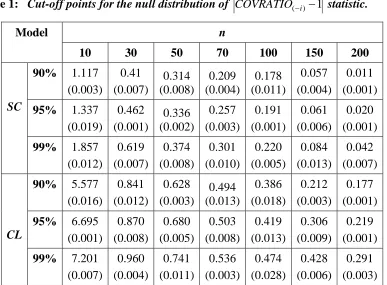
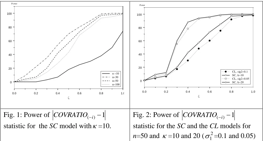
The process is repeated 2000 times and the power of performance is calculated as the percentage of the correct detection of the contaminated observation at position d. The results of simulation study show that: in all cases, the power of performance is an increasing function of the contamination level , Figure 1 shows the power of performance is a decreasing function of the sample size n. On the other hand, Figure 2 shows that the COVRATIO statistic for the (SC) model performs more efficient than the (CL) model when the association between the circular random variables is linear.
Fig. 1: Power of COVRATIO(i)1
statistic for the SC model with=10.
Fig. 2: Power of COVRATIO(i)1
statistic for the SC and the CL models for
n=50 and =10 and 20 (12=0.1 and 0.05)
Unlike the procedure used by Hussin and Abuzaid (2012) for contaminating the real and imaginary parts in (CL) model separately, we contaminate the generated data before the
0.0 0.2 0.4 0.6 0.8 1.0
0 20 40 60 80 100
n =10 n=30 n=50 n=100
P ower
0.0 0.2 0.4 0.6 0.8 1.0
0 20 40 60 80 100
CL, sig2=0.1 SC, k=10 CL, sig2=0.05 SC, k=20
reasonable and consistent where the power starts at almost zero when =0 and approaches to 100% when goes to 1.
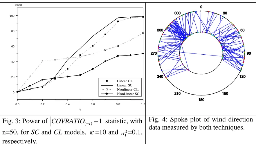
Contrasting with the case when the circular variables are linearly correlated, Figure 3 shows that the COVRATIO statistic for the (SC) model performs less efficient than the (CL) model when the association is nonlinear.
Fig. 3: Power of COVRATIO(i) 1 statistic, with
n=50, for SC and CL models, =10 and 2 1
=0.1, respectively.
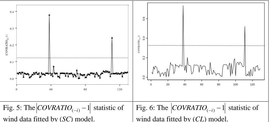
Fig. 4: Spoke plot of wind direction data measured by both techniques.
4. Numerical Example
A real data set consisting of 129 pairs of observations of wind direction are recorded by two different instruments: an HF radar system and an anchored wave buoy. Figure 4 shows the spoke plot of wind direction data (Zubairi, et al., 2008). The inner ring represents the HF radar while the outer ring represents the anchored wave buoy. Since almost all the lines do not cross the inner circle, it means that the data are highly correlated with estimated correlation parameter rˆc 0.952. Furthermore, there are only two lines crossing the inner ring, which are associated with observations number 38 and 111. This indicates that the pairs corresponding to the two observations may be influential. The data are fitted by the (SC) model giving Y =0.1250.989X (mod2),
with ˆ11.48, and the (CL) model is given by
cosYisinY
7.5271040.977
cosXisinX
with ˆ2 0.148.The values of COVRATIO i 1 for the (SC) and the (CL) models are obtained and
given in Figure 5 and Figure 6, respectively. The statistics are able to define two observations as influential points which are 38 and 111. To investigate the effect of these two points they are deleted and the data are refitted using the (SC) and the (CL) models. The values of parameter estimates and their standard errors are given in Table 2. It is noticeable that for both models the estimates of intercept and slope become closer to zero
0.0 0.2 0.4 0.6 0.8 1.0
0 20 40 60 80 100
Linear LC, n=50 Linear SC, n=50 Nonlinear LC, n=50
Text NonLinear SC, n=50 Power
and one, respectively. The standard error of the slope parameter in the (SC) model for the reduced data is less than the full data. On the other hand, for the (CL) model the standard error is almost the same. This indicates the efficiency of the COVRATIO statistic for the (SC) model more than the (CL) model in the considered data.
Fig. 5: TheCOVRATIO(i)1 statistic of
wind data fitted by (SC) model.
Fig. 6: The COVRATIO(i) 1 statistic of
wind data fitted by (CL) model.
Table 2: Parameters estimates of the (SC) and the (CL) models associated with the standard error
Model SC CL
Parameter Full data Reduced data Full data Reduced data
ˆ 0.125 (0.072) 0.104 (0.059) 7.52 5
10
(2.5105) -0.90105(2.0105) ˆ 0.989 (0.017) 0.999 (0.014) 0.977(1.88 2
10
) 1.00 (1.88102)
ˆ 11.468 (0.004) 16.739 (0.001) - -
2
ˆ
- - 0.148 (8.38 3
10
) 0.118 (8.17103)
Conclusion
COVRATIO statistic as an identifier of the influential points in functional relationship models of circular variables is derived and tested for two types of models. If two circular variables are correlated linearly, then the COVRATIO statistic of the (SC) model performs better than the (CL) model, vice versa for other types of association.
The contamination procedure of the (CL) model has shown a reasonable performance compare to the procedure used previously by Hussin and Abuzaid (2012). The application of the proposed statistics for both models on wind data has shown a consistent conclusion of detecting two points as influential points.
0 40 80 120 0.0
0.1 0.2 0.3 0.4
|C
O
V
R
A
T
IO
(i
)
-1
|
0 20 40 60 80 100 120
0
.0
0
.2
0
.4
0
.6
|C
O
V
R
A
T
IO
(-i)
References
1. Caires, S. and Wyatt, L.R. (2003). A linear functional relationship model for circular data with an application to the assessment of ocean wave measurements.
J. Agric. Biol. Environ. Stat., 8 (2), pp. 153-169.
2. Hassan, S.F., Zubairi, Y.Z. and Hussin, A.G. (2010). Analysis of missing values in simultaneous linear functional relationship model for circular variables.
Scientific Research and Essays, 5(12), pp. 1483-1491.
3. Hussin, A.G., Abuzaid, A., Zulkifili, F. and Mohamed, I. (2010). Asymptotic covariance ad detection of influential observations in a linear functional relationship model for circular data with application to the measurements of wind directions. Science Asia, 36, pp. 249-253.
4. Hussin, A. G. and Abuzaid, A. (2012). Detection of outliers in functional relationship model for circular variables via complex form. Pakistan Journal of Statistics, 28(2), pp. 205-216.
5. Hussin, A.G. (2008). Asymptotic properties of parameters for linear circular functional relationship model. Asian Journal of Mathematics and Statistics, 1 (2), pp. 118-125.
6. Fisher, N.I. (1993). Statistical Analysis of Circular Data. Cambridge University Press.
7. Belsley, D.A., Kuh, E. and Welsch, R.E. (1980). Regression Diagnostics: Identifying influential data and sources of collinearity, New York: John Wiley & Sons.
8. Abuzaid, A., Mohamed, I., Hussin, A.G. and Rambli, A. (2011). COVRATIO statistic for simple circular regression model. Chiang Mai J. Sci.38 (3), pp. 321-330.
9. Jammalamadaka, S.R. and SenGupta, A. (2001). Topics in Circular Statistics,
Singapore: World Scientific Press.
10. Singh, H., Hnizdo, V. and Demchuk, E. (2002). Probabilistic model for two dependent circular variables. Biometrika, 89, pp. 719–723.
11. Best, D. J. and Fisher, N. I. (1979). Efficient simulation of the von Mises distribution. Journal of the Royal Statistical Society. Series C, 28(2), pp. 152-157. 12. Zubairi, Y.Z., Hussain, F. and Hussin, A.G. (2008). An Alternative Analysis of