Automatic Weight Selection Algorithm for
Designing H Infinity controller for Active
Magnetic Bearing
Sarath S Nair
Department of Electrical Engineering, Amrita Vishwa Vidyapeetham University, Coimbatore, Tamil Nadu, 641105, India
Abstract:- In recent times active magnetic bearing has got wide acceptance in industries and other special systems. Current researches focus on improving the disturbance rejection properties of magnetic bearings to work well in industrial environment. So far many controllers have been developed to control the system, of
which the H∞ controller is found to guarantee robustness and performance. In this paper an automatic weight
selection algorithm is proposed to design robust H Infinity controller automatically for active magnetic bearing system and detailed disturbance analysis is done. This paper focuses on the controller implementation point of view and analyses the variation in control current, peak responses and steady state error of the developed controller. Comparison with a well tuned PID controller shows the efficacy of H infinity controller designed using the proposed algorithm.
Keywords: Active magnetic bearing, H∞ control, Weight functions.
I. Introduction
Active magnetic bearing (AMB) is an advanced mechatronic device having wide spread applications in turbo machineries. It is a collection of electromagnets producing a magnetic field to support a rotating iron shaft without any physical contact. AMBs are widely used in industries because of its advantages such as no mechanical contact and lubrication. Active magnetic bearings are open loop unstable systems and so the stabilization of the system can only be done by feedback control. Many control strategies [6] have been developed which enable the bearing to be used for a variety of applications including high speed machining [6],[13],[15] and fly wheel energy storage.
The magnetic bearing under any advanced control strategy need to work in highly adverse operating conditions.
Many types of disturbances act on AMB when working in industrial environments. Robust H∞ control can
provide a perfect control to linear systems and high robustness to stabilize in adverse operating conditions like parameter change, high disturbance environment actuator saturation and model uncertainty. H Infinity control provides very high disturbance rejection, guaranteeing high stability for any operating conditions. Mixed weight H Infinity controllers can provide a closed loop response of the system as per design specifications. The design specification includes model uncertainty, disturbance attenuation at higher frequencies, required bandwidth of the closed loop plant etc. But in implementation point of view, H Infinity controllers are of very high order and also the control effort requirement may be large. Most of the time the design may be system specific and so requires specific analysis based on the system. H infinity controller can be synthesized using different techniques, but now a day’s, H infinity loop shaping is gaining very high acceptance since the performance requirements can be incorporated in the design stage as performance weights. In the H infinity loop shaping technique a linear plant model is augmented with certain weight functions like sensitivity weight function, complementary weight function and control sensitivity weight function so that the closed loop transfer function of the plant will have the desired performances. From the literature it can be understood that there exists no specific criterions for the selection of these weights and most of the time they are system specific. It requires high analytical skills for a control engineer to design these weights which makes H infinity control to be inferior to other control strategies.
little about the analysis of responses. Also the efficacy of H Infinity controller to replace an industry standard PID controller can be explained only after doing analysis on the responses of the system. The effect of H Infinity controller on various system responses like peak overshoot, steady state error needs to be investigated in detail.
In this paper an automatic weight selection algorithm is proposed for designing H Infinity controller for an AMB model and its performance responses are compared with a well tuned PID controller. Detailed mathematic model of the magnetic bearing is developed and the variation of peak overshoot, dynamic compliance and the steady state error for various load conditions are analyzed. The H infinity controller synthesized using the proposed algorithm is tested for its efficacy using an illustrative example. The analysis on robustness and performance of the system is done by taking the singular value responses and robustness indicator plots.
The paper is organized as mentioned below. The technology of active magnetic bearing is described in section
II. The section III describes the general robust H∞ control theory followed by its design using proposed
automatic weight selection algorithm in sections IV. Design examples are shown in section V followed by its analysis in section VI. The implementation details of the proposed methodology is discussed in section VII followed by the conclusion in section VIII.
II. Active Magnetic Bearing System
In active magnetic bearing shown in fig (1) the mechanical iron shaft is supported by a set of attractive forces provided by the electromagnets. When a current is passed through the electromagnet it produces a magnetic field and attracts an iron shaft in its vicinity. The attracting force produced by the electromagnet is a function of the current passing through it and the perpendicular distance between the pole faces and the iron shaft. The net force produced by a differential actuator in a plane is equal to the difference of the forces produced by the electromagnets. Thus the shaft of the AMB is stabilized at a particular point by the combined effect of the forces produced by the actuators in all the planes. A perturbation current is added or subtracted from the bias current to produce a net force to bring the shaft to its reference frame.
Fig (1) Active Magnetic Bearing [16]
II. (A) Mathematical Modeling
Normally a magnetic bearing consists of four electromagnets providing movements of the shaft in 2 degrees of
freedom (D.O.F). Each DOF consists of a differential actuator providing forces f1 and f2 in opposite directions.
The total force ‘f ’ acting on the shaft will be the algebraic sum of the two forces given by the equation (1).
(1)
When there is a disturbance the shaft displaces by some position and the current in the magnetic bearing coils
need to be adjusted for compensating the effect of disturbance. Let ‘io’ be the bias current and ‘ix’ be the control
current during the presence of a displacement ‘x’ of the shaft from equilibrium position. The total force ‘f’ exerted by the magnetic bearing on the shaft can be written in terms of values of current and displacement as
(2)
Where ‘K’ is
2 0
4
N A
K
Linearizing the equation (2) in the equilibrium point (i0 ,x0),
(3)
With,
(4)
The shaft suspended by the magnetic bearing can be considered as a spring mass, damper system. Let ‘m’ be the mass of the shaft and ‘x’ be the displacement of the shaft from the equilibrium point in the presence of an
external disturbance of magnitude ‘fext’. Then the mass balance equation of the system can be written as
(5)
Equation (5) shows the differential equation of the magnetic bearing in a single degree of freedom. To find out the open loop transfer function of the plant model,
The equation (5) is re arranged in transfer function domain as
(6)
For a magnetic bearing the position or displacement x is fed back and the controller Gc(S) which provides the
control current I. The relationship between the feedback signal and control current is given as
(7)
Re arranging equation (6) we get
2 2
1 2
0
(
)
A
f
f
f
B
B
2 0 2 0 2 0 2 0 2 1)
(
)
(
)
(
)
(
x
x
i
i
x
x
i
i
K
f
f
f
x x0 0 0 0
( , )
i(
)
x(
)
f
f i x
k i i
k x
x
2 2 2
0 0
2 3
2
2
,
i x
N Ai
N Ai
K
K
x
x
0
)
,
(
)
(
)
(
)
(
)
(
)
,
(
)
(
0 0 0 0 2 2 0 0 0 0 2 2 2 1 2 2
x
i
f
because
f
x
x
k
i
i
k
dt
x
d
m
x
x
k
i
i
k
x
i
f
f
dt
x
d
m
f
f
f
dt
x
d
m
ext x i x i ext ext ext xi
I
s
k
X
s
F
k
s
X
ms
2(
)
(
)
(
)
)
(
)
(
)
(
s
G
s
X
s
(8)
The above closed loop transfer function of the plant is compared with the general closed loop system to find the open loop transfer function of magnetic bearing system.
Standard closed loop transfer function is given as
G(s) = (9)
By connecting the two equations (8) and (9) the open loop transfer function of a linearized model of active magnetic bearing is
(10)
In the transfer function
K
istands for the damping coefficient,K
x is the stiffness coefficient and ‘m’ is themass of the shaft suspended by the bearing, ‘N’ is the number of turns of copper windings in each electro magnet, ‘A’ is the area of cross section of the pole face.. The transfer function is obtained by linearizing the force balance equation of the magnetic bearing under dynamic conditions.
III. HInfinity control
All devices are common to have some uncertainties which are difficult to measure and thus to appropriately model, such as the digital implementation and amplifiers delay, or sensor offsets [10]. To deal with these
characteristics and get a robust control H∞based is proposed. Robust control theory was first developed by
Zames and it addresses both the performance and stability criterion of a control system. The robust control provides better closed loop control than a PID control.
Let
G
(
s
)
is the open loop transfer function of the plant andK
(
s
)
is the controller transfer function such thatthe closed loop system perform robustness and good performance. The controller
K
(
s
)
will be derived keepingthree criterions. They are
III.1. Stability criterion:- It states that the roots of the characteristic equation
1
G
(
s
)
K
(
s
)
0
should lie in the left half side of s plane.III.2. Performance Criterion:- It states that the sensitivity
)
(
)
(
1
1
)
(
s
K
s
G
s
S
to be small for allfrequencies where disturbances and set point changes is large. Sensitivity is the transfer function between the output and disturbances of a system.
III.3. Robustness criterion:- It demands for stability and performance to be maintained not only for the nominal model but also for a set of neighboring plant models that result from unavoidable presence of modeling
errors. Robust H∞ controllers are developed to provide a highly robust control environment to linear systems.
The detailed design procedure for H∞control of linear system is described in works done by Guangzhong Cao,
Suxiang Fan, Gang Xu [1], Arredondo and J. Jugo [2], Zdzislaw Gosiewski, Arkadiusz Mystokowski [3].
In general the H∞norm of a transfer function, F, is its maximum value over the entire frequency range, and is
denoted as
Where,
is the largest singular value of a transfer function. The objective of the synthesis is to design acontroller such that the H∞norm of the plant transfer function is bound within limits. Different methods are
available for the synthesis of the H∞controllers viz two transfer function method and three transfer function
)) ( (
sup
F j
method. Two transfer function method have less computational complexities and so is considered for H∞
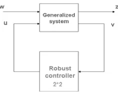
controller synthesis in this paper.The robust control problem can be formulated as drawn as in fig (2).
Fig (2) Robust Control Problem
In the traditional H∞controller synthesis two transfer functions are used which split a complex control problem
into two separate sections, one dealing with stability, the other dealing with performance. The sensitivity function, S, and the complementary sensitivity function, T, are used in the controller synthesis and are given by equations (11) and (12).
Sensitivity function is the ratio of output to the disturbance of a system and complementary sensitivity function is the ratio of output to input of the system.
(11)
(12)
Where ‘w’ is the vector of all disturbance signals, ‘z’ is the cost signal consisting of all errors. ‘v’ is the vector consisting of measurement variables and ‘u’ is the vector of all control variables.
The controller design problem is then to find a controller K, which, based on the information in v, generates a
control signal u, which counteracts the influence of w on z, thereby minimizing the closed loop norm w to z. It
is done by bounding the values of
(
S
)
for performance(
T
)
for robustness. By minimizing the norm) ( minN K
K (13)
Where,
T W
S W N
t
s (14)
Where
W
s andW
t are the weight functions assigned to the problem by the designer. The ultimate aim of therobust control is to reduce the effect of disturbance on output. So sensitivity S and the complementary function
T are to be reduced. For obtaining that it is enough to reduce the magnitude of
S
andT
. This can be done bymaking
) ( 1 ) (
jw W jw S
s
and
) (
1 jw W T
t
Where Ws and Wt are the weight function assigned by the designer.
s
W
is the performance weighting function to limit the magnitude of the sensitivity function andW
t is therobustness weighting function to limit the magnitude of the complementary sensitivity function This technique called as loop shaping technique is widely used for selecting the weight functions for the synthesis of the controller and is shown in Fig (3) and Fig (4).
GK GK T
1
GK S
Fig (3) Required nature of frequency plots
Fig (4) Required nature of frequency plots
As mentioned earlier the robust controller is synthesized in order to make the H∞norm of the plant to be as low
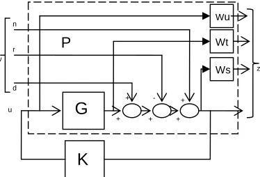
as possible. In order to obtain this condition three weight functions are added to the plant for loop shaping. The weight functions are in fact lead-lag compensators which can shape the frequency response of the system in the desired way. Loop shaping is done to make the frequency response of the plant with the weight functions to come in the desired manner. Loop shaping can be done in many ways. In loop shaping the parameters of the weight functions are changed to make the frequency response of the whole system to remain within limits. The control synthesis requires the plant transfer function, controller transfer function and the various weight functions to augment together. Thus an augmented plant model is made as shown in Fig (5).
Fig (5) Augmented Plant model for the synthesis of H∞controller.
The normalized frame of the plant is
u w
G I
G w
w G w w
e y w
u w
e w
t u s s
t u s
0
0 (15)
Where, U=K*e
After determining the weights
W
t andW
s, the plant can be determined asd r n
G
K
Ws Wt
+
+ - +
+ +
P
w
z
u
22 21 2 12 11 1 2 1 0 0 D D C D D C B B A G I G w w G w w P t u s s (16)
The equation (17) is written as a mixed sensitivity problem in terms of (15) & (16) as
T W R W S W P t u s (17)
Mixed sensitivity problem is to find a rational function controller K(s) and make the closed loop system stable and satisfy T W R W S W P t u s min
min (18)
Where P is the transfer function from w to Z i.e
zw
T (19)
Where, Tzw P is the cost function. According to the
minimum gain theorem, make the H∞norm of
T
zw less than unity.i.e, 1 min min T W R W S W T t u s zw (20)
Thus a stabilizing controller K(s) is achieved by solving the algebraic riccatti equations minimizing the cost
function γ.
As mentioned in the robust control theory the synthesis of the controller requires the selection of two weight functions. The work done by Jiankun Hu, Christian Bohn, H.R. Wu [5] suggests some methods for the selection of these weight functions for different plant transfer functions. The works shown in reference [8] also describes some ways for designing robust controller for uncertain plants. In all these design procedure the weighting
functions are selected using trial and error method and later the H∞ controller is synthesized by loop shaping
technique. The main draw back in this type of synthesis is that the train and error procedure may not end up in a stabilizing controller.
The open loop transfer function of the active magnetic bearing shows that it consists of two poles out of that one pole lies in the right hand side of the S plane making it unstable. The weight functions for such types of systems are very difficult to determine. No previous work describes the method to select weight functions for transfer functions of the type of magnetic bearings. More over the work in [4] describes some of the difficulties involved in selecting the weight functions for robust control design. From all these previous works it can be concluded that no straight rules are available for such types of plants till now for the selecting the weight functions. Trial and error method is adopted for loop shaping to find out the controller, making the whole problem solving method a tedious and laborious job. Due to these problems in the weight selection and loop
shaping technique, finding an algorithm is difficult in the design of H∞controller.
IV. Automatic Weight Selection Algorithm
The synthesis procedure of H∞controller can be done only by selecting proper weight functions. The selection
purely depends on the plant model. There are no hard and fast rules for selecting the performance weight function and the robustness weighting functions. An iteration work with assumed initial values is conducted to find out the weight functions. It is very difficult to achieve simultaneously meet all the requirements for the
synthesis of robust controller. After many trial and error methods, a systematic procedure for the synthesis of H∞
Even though there are no methods available for selecting the transfer functions for weight functions, certain generalization can be done by understanding the loop shaping procedure. Such an empirical formula to
determine the performance and robustness weights for a general H∞ control problem is suggested by skojested
and the work in [1], and is given in equations 13 and 14. The main draw back in this is that there are so many parameters to be fixed for determining the weight functions.
(21)
(22)
Where Ws is the performance weighting function, ‘
w
b’ is the cut off frequency, ‘M’ is the gain for highfrequency disturbances and ‘A’ is the gain for low frequency control signal and L is a constant.
w
b is thefrequency which differentiates the high frequency disturbance signal and the low frequency control signal. The plots, Fig (2) and Fig (3) show the nature of
) ( 1
jw Ws
, S and ) (
1
jw Wt
, T to be satisfied for the synthesis of H∞
controller. This can be made by closely shaping the ) ( 1
jw Ws
and ) (
1
jw Wt
plot. This loop shaping technique
consists of adjusting the various parameters of the weight functions. A generalization is made on how these
parameters are to be varied to closely shape the curves to make a robust H∞ controller synthesis algorithm. The
flow chart of the automatic weight selection algorithm is shown in fig (6).
The automatic weight selection algorithm takes the transfer function of active magnetic bearing and plots the bode plot of open loop transfer function. The cross over frequency ‘wb’ required by the closed loop transfer function is inputted and it computes the initial form of sensitivity weight function and complementary weight function. The initial form of sensitivity weight function is designed by putting the values of ‘A’ and ‘M’ as 0.1 and 1 respectively in the equation given in (21). The initial form of complementary weight function is designed by putting the value of ‘L’ as 0.01. After calculating the initial forms of the weight functions, the H infinity controller is designed by solving the Algebraic Riccatti equations using ‘hinfsyn’ command in MATLAB. The objective of the algorithm is to modify the weights until the various performance criterions specified in robust control theory is met. As per the robust control criterion, the algorithm searches for a minimum value of cost
function γ along with shaping the closed loop responses of sensitivity function, and complementary sensitivity
function. Once the first iteration is over the algorithm checks whether the frequency response of sensitivity function ‘S’ falls less than inverse of frequency response curve of sensitivity weight function ‘Ws’. If not, the algorithm makes modification in the values of A and M as shown in the flow chart. Once the loop shaping of sensitivity weight function ‘S’ is done, the algorithm tries to shape the response of complementary weight function ‘T’ fall less than the frequency response of complementary sensitivity function ‘Wt’ by adjusting the value of ‘L’ as shown in flowchart.
A w s
w M s Ws
b b
/
) 1 5 . 0 ( 2
1
Fig (6) Automatic weight selection algorithm
When the performance criterion and robustness criterion are met, the algorithm tries to reduce the value of cost
function γ to be less than unity. This is done by adjusting the values of A, M and L as shown in flow chart.
V. Design Example
In order to validate the selection procedure of weighting functions, active magnetic bearing of different
specifications are taken and Robust H∞ controllers were designed. The selection procedure and the algorithm
are coded in MATLAB and executed. The algorithm was found to converge for different specifications of
magnetic bearings and the synthesized H∞ controller met the robustness and performance criterion. The
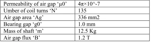
specification for a prototype used for validation of the above strategy is shown in the table I. The specifications given in table 1 is the experimental model developed in the laboratory for testing as a part of this project.
Table (I) Specification of Magnetic Bearing example I
Permeability of air gap ‘µ0’ 4π×10^-7
Umber of coil turns ‘N’ 135
Air gap area ‘Ag’ 336 mm2
Bearing gap ‘g0’ 1.0 mm
Mass of shaft ‘m’ 12.5 Kg
Air gap flux ‘B’ 1.2 T
The algorithm written in MATLAB returned the following H∞ controllers meeting the criterions. The transfer
Damping Constant, Ki = 27 N/A
Stiffness constant, Kx = 1.9261e+005 N/m
27
Plant Transfer function: = ---
(12.5S2-1.9261e+005)
1.308e013 s^3 + 4.705e015 s^2 + 4.753e017 s + 1.153e019
K(s)= ---
s^4 + 1.063e005 s^3 + 3.119e009 s^2 + 9.236e012 s + 4.61e013 (23)
The controller transfer function in discrete form is
-4.887e006 z^3 + 5.185e006 z^2 + 4.299e006 z - 4.598e006 K(z) = --- z^4 - 1.722 z^3 + 0.7256 z^2 - 0.00362 z + 2.429e-005
(24) Sampling time: 0.0001
The weighting functions designed by the algorithm are
0.33333 (s+300)
W(s) = --- (25)
(s+5)
(s+100)
W(t) = --- (26)
(s+200)
With GAMMA= 0.7772
VI. Analysis of the H∞ control
To provide global acceptance to the H∞ control for active magnetic bearing it should stabilize the highly
complex plant under all operating conditions. Active magnetic bearings are non linear systems, so the H infinity controller developed using a linear model should stabilize the actual plant under all operating conditions. For that a non linear model is developed in MATLAB/SIMULINK as shown in fig (7) and various tests and analysis
are conducted to understand the performance of magnetic bearing under the H∞ control developed by the
Fig (7) Active Magnetic Bearing Model
A. Stability Analysis
Stability analysis is done to ensure the stability of operation of active magnetic bearing under various conditions. The bode plot of the closed loop sensitivity function of robust controlled active magnetic bearing given in example 1 is shown in fig (8). The plot shows that the system is stable for a wide range of frequencies for both the bearing specifications.
-40 -30 -20 -10 0
T
o
: O
u
t(
1
)
-180 0 180
T
o
: O
u
t(
1
)
-100 -50 0
T
o
: O
u
t(
2
)
100
101
102
103
104
105
106
-360 0 360
To
: O
u
t(
2
)
Bode Diagram
Frequency (rad/sec)
M
agni
tu
de (
d
B
)
; P
has
e
(de
g)
Sensitivity Function
Complementary sensitivity function
Fig (8) Bode plot of H∞ controlled AMB(example 1)
B. Performance Analysis
0 0.05 0.1 0.15 0.2 0.25 0.3 0.35 0.4 0.45 0.5 -2
0 2 4 6 8 10 12 14x 10
-5
time(sec)
di
s
pl
ac
em
ent
(
m
m
)
Set Point Tracking
PID Control Generalized H Infinity Control Set Point Tracking
Fig (9) Step response
0 0.02 0.04 0.06 0.08 0.1 0.12 0.14 0.16 0.18 0.2 -0.8
-0.6 -0.4 -0.2 0 0.2 0.4 0.6 0.8
time (sec)
d
isp
la
ce
m
e
n
t (
m
m
)
Set Point Tracking-Control Current
PID Control Generalized H Infinity Control Control Current variation of AMB for a set point change
Fig (10) Control current for unit set point change
0 0.1 0.2 0.3 0.4 0.5 0.6 0.7 0.8 0.9 1
0 1 2 3 4 5 6 7 8x 10
-6
time(sec)
D
isp
la
ce
m
e
n
t (
m
m)
Disturbance rejection of H infinity control
50 % load as disturbance 30 % load as disturbance 10 % load as disturbance Disturbance Rejection of H Infinity Control
Fig (11) Disturbance response with H Infinity Control
0.08 0.1 0.12 0.14 0.16 0.18 0.2
-4 -3.5 -3 -2.5 -2 -1.5 -1 -0.5 0 0.5 1
Control Current for disturbance rejection
10 % load 30 % load 50 % load H Infinity control Currents for under variou step disturbances
0 0.05 0.1 0.15 0.2 0.25 0.3 0.35 0.4 -1
0 1 2 3 4 5 6x 10
-4
time (sec)
d
is
p
la
c
e
me
n
t (
mm)
Disturbance Rejection of PID control
10 % load as disturbance 30 % load as disturbance 50 % load as disturbance Disturbance Rejection of PID Control
Fig (13) Disturbance response with PID control
0 0.05 0.1 0.15 0.2 0.25 0.3 0.35 0.4 0.45 0.5
-7 -6 -5 -4 -3 -2 -1 0 1
time (sec)
c
o
n
tro
l c
u
rr
e
n
t (
A
)
Control current for disturbance rejection
10 % load 30 % load 50 % load PID control current for disturbance rejection
Fig (14) PID Disturbance rejection control current
C. Robustness Analysis
Robust H∞ controller developed not only operates on the known AMB plant in a stable environment, but also
provides good control for a set of nearbyuncertain plants [8]. The system must be robust enough to provide
good performance and stability over the uncertainty. Singular values are a good measure of the system robustness. The Fig (15) plots the singular value plot of the system with H infinity control and PID control.
10-1
100
101
102
103
104
105
106
-100 -80 -60 -40 -20 0 20
Singular Values of AMB example 1
Frequency (rad/sec)
S
ing
ul
a
r V
al
u
es
(
dB
)
S_Hinfinity T_Hinfi S_pid T_pid
Fig (15) Singular Value Plot
The figure shows the singular values of sensitivity function, complementary sensitivity function with H infinity control and PID control. The singular values of sensitivity function and complementary sensitivity function of AMB plant controlled under H infinity control lies below the zero gain for range of operating frequencies. A comparison between the plots of closed loop sensitivity function with PID control ‘S_PID’ and closed loop sensitivity function with H infinity control ‘S_H Infinity’ shows that for the range of operating frequencies from
100 to 104 rad/sec , singular values S_H infinity is less than singular values of S_PID. From this it can be
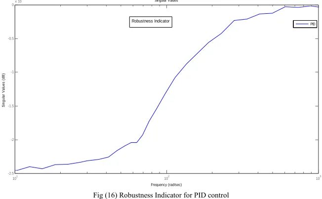
In most of the cases the disturbance to the plant acts as an uncertainty. For SISO systems it is known that singular values of sum of sensitivity function and complementary function can be taken as a good measure of robustness indicator. The minimum the value of maximum singular value better the control.
i.e.
(19)
The robustness indicator plot drawn for the AMB given in example 1 for PID and H infinity controller developed by the procedure is given below. It shows that the magnitude of the singular values is very less for all values of frequencies for H infinity control when compared with PID control. This again confirms the disturbance rejection property of the H infinity controller developed by the method. The robustness indicator plots are given in fig (16) & fig (17).
101 102 103
-2.5 -2 -1.5 -1 -0.5 0
x 10-13 Singular Values
Frequency (rad/sec)
S
ingul
ar
V
al
ues
(
dB
)
PID Robustness Indicator
Fig (16) Robustness Indicator for PID control
A closer look at the plots shows that the magnitude of the robustness indicator for PID controller is higher than the magnitude for H infinity controlled system synthesized using the proposed algorithm.
100 101 102 103 104 105
-20 -15 -10 -5 0 5x 10
-9 Singular Values
Frequency (rad/sec)
S
ing
ul
a
r Val
u
es
(
d
B)
H infinity control
Robustness Indicator
Fig (17) Robustness Indicator for H∞ control
D. Dynamic Compliance
The variation of the control current with various values of load on the bearing in example 1 is shown in fig (18) & fig (19). From the plot it can be seen that the control effort at steady state is same for both H infinity and PID control.
) ) ( ) ( (
max
S j T j
Fig (18) Variation of PID control current with load
Fig (19) Variation of H infinity control current with load
The fig (20) is the variation of the steady state error of the shaft after it is settled under H infinity and PID control. The plot shows that the steady state error is higher for all values of load under H infinity control than PID control where as the plot in fig (21) is the variation of peak overshoot when there is a set point change or disturbance to the plant. As per this plot, the peak overshoot is less for H infinity control.
Fig (20) Variation of steady state error with load
Fig (21) Variation of peak overshoot with load
VII. Hardware Implementation
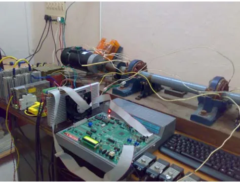
freedom in x axis and in y axis. Four position sensors are placed to get the position signals in each degree of freedom. The signals are converted to digital signals inside the DSP processor. The transfer function of the robust H infinity control using automatic weight selection algorithm is implemented as difference equation in digital signal processor. A graphical user interface (GUI) shown in fig (23) developed in MATLAB software takes the details of the bearing and synthesize H infinity controller using the algorithm. Using the GUI minimum effort is required by the designer to synthesize the controller. The DSP processes the position signals of each DOF using the respective difference equation of that axis and provides the manipulated variable as variations in duty ratio of PWM signals. The PWM signals switch the respective power electronic trans-conductance amplifier to power up the coil of the electromagnets in each DOF. The voltage variations indicated by the 8 PWM signals are converted to current pulses to energize the bearing coils.
Fig (22) Hardware setup of Active magnetic bearing with H Infinity control
Fig (23) GUI for designing H infinity controller using Automatic Weight Selection Algorithm
VIII. Conclusion
In this work an automatic weight selection algorithm is proposed for synthesizing Robust H∞ controller for
active magnetic bearing systems. In H infinity control synthesis using loop shaping technique two weight functions are to be designed for shaping the closed loop characteristics of the system. The selection of these two weight functions are normally a trial and error procedure or requires detailed analysis of the system requirements. In this paper a novel automatic weight selection algorithm is proposed, by which the H infinity controller can be synthesized automatically. The algorithm automatically synthesizes the weight functions meeting all the requirements of robust control for active magnetic bearing. A detailed analysis of the developed
H∞ controller for stability, performance and robustness has been made for both magnetic bearing. The results
overshoot is less for H∞ control than PID control. Robustness indicator plots shows that the proposed algorithm could synthesis H infinity controller that can provide high disturbance rejection property to magnetic bearings than a well tuned PID control. The detailed analysis in steady state and transient conditions like load variations provide a good sign that the proposed algorithm could control magnetic bearing with high robustness and performance with minimum time and complexity in controller design.
References
[1] Guangzhong Cao, Suxiang Fan, Gang Xu “The Characteristics Analysis of Magnetic Bearing Basedon H-infinity Controller”, Proceedings of the 51th World Congress on Intelligent Control and Automation, June 15-19, 2004, Hangzhou, P.R. China
[2] Arredondo and J. Jugo, “Active Magnetic Bearings Robust Control Design based on Symmetry Properties”, Proceedings of the 2007 American Control Conference,
[3] USA, July 11-13, 2007
[4] Zdzislaw Gosiewski, Arkadiusz Mystokowski, “Robust control of active magnetic bearing suspension: Analytical and experimental study”, Mechanical systems and Signal Processing (2007)
[5] R.W. Beaven, M.T. Wright and D.R. Seaward, “Weighting function selection in the H∞ design Process”,Control Eng. Practice, Vol. 4, No. 5, pp. 625-633, 1996
[6] Jiankun Hu, Christian Bohn, H.R. Wu, “Systematic H∞ weighting function selection and its application to the real-time control of a vertical take-off aircraft”, Control Engineering Practice 8 (2000) 241-252
[7] Carl R. Knospe, “Active magnetic bearings for machining applications, Control Engineering Practice 15 (2007) 307–313
[8] Mark Siebert, Ben Ebihara,Ralph Jansen, Robert L. Fusaro and Wilfredo Morales, Albert Kascak, Andrew Kenny, “A Passive Magnetic Bearing Flywheel”, NASA/TM—2002-211159,36th Intersociety Energy Conversion Engineering Conference cosponsored by the ASME, IEEE, AIChE, ANS, SAE, and AIAA Savannah, Georgia, July 29–August 2, 2001,
[9] C Verde & J Flores, “Nominal model selection for robust control design”, proceedings of the American control conference, seatle, Washington, 1996.
[10] W. Beaven, M.T. Wright and D.R. Seaward, “Weighting Function selection in the H∞ design process”, control eng. practice, vol. 4,
no. 5, pp. 625-633, 1996
[11] S. Engell, “Design of robust control systems with time-domain specifications”, control eng. practice, vol. 3, no. 3, pp. 365-372, 1995
[12] Ulrich schonhoff and Rainer Nordmann, “An H ∞ -weighting scheme for PID like motion control”, proceedings of the 2002 IEEE international conference on control applications, September 18-20, 2002, Glascow, Scotland, U.K
[13] Didierh Enrion', Michael Sebek and Sophie Tarbouriech', “Algebraic approach to robust controller design: A geometric interpretation”, Proceedings of the american control conference philadelphia, pennsylvania june 1998
[14] Carl r. knospe roger l. fittro, “Control of a high speed machining spindle via µ-synthesis”, Proceedings of the 1997 IEEE International conference on control applications hartford, ct - october 5-7, 1997
[15] Z F Jiang, H C Wu, H Lu, C R Li, “Study on the Controllability for Active Magnetic Bearings”, Journal of Physics: Conference Series 13 (2005) 406–409
[16] M.H.Kimman,H.H.LangenJ.vanEijkR.MunnigSchmidt, “Design and Realization of a Miniature Spindle Test Setup with Active Magnetic Bearings”,1-4244-1264-1/07/ ©2007 IEEE
![Fig (1) Active Magnetic Bearing [16]](https://thumb-us.123doks.com/thumbv2/123dok_us/9629818.1490995/2.612.213.418.388.561/fig-active-magnetic-bearing.webp)