Probabilistic Analysis of an Automatic Power Factor Controller with variation in Power Factor

(1)

Probabilistic Analysis of an Automatic

Power Factor Controller with variation in

Power Factor

P.K. BHATIA1

Department of Applied Mathematics, D.C.R.U.S.T, Murthal, Haryana, India

[email protected]

ROOSEL JAIN2

Department of Applied Mathematics, D.C.R.U.S.T, Murthal, Sonepat, Haryana, India

[email protected]

GULSHAN TANEJA3

Department of Mathematics, M.D. University, Rohtak, Haryana, India

[email protected]

Abstract:

In the present study, the probabilistic analysis of an automatic power factor controller (APFC) system working in industry/factory is investigated. The power factor correction of electrical loads and energy losses due to poor power factor are the problems common to all industrial companies. Therefore, the study of APFC unit is of great importance. Initially, the system is operative with controlled power factor. Then it may transit to state with power factor not controlled. On the failure of the system, an inspection is carried out to detect the type of failure. The system may fail due to Fuse blown off, Transformer burnt, Programming problem, Output relay faulty. In case of the first two types of failure the components are replaced and corrected; while in last two types of failures the problem is repaired and corrected. The system remains in up state with power factor controlled and power factor not controlled. The system is analyzed by making use of regenerative point technique. The various measures of system effectiveness are obtained including the profit incurred to the system. Graphs have been plotted to depict the behavior of the profit with respect to revenue/loss per unit up time when power factor controlled and when power factor not controlled, cost per unit replacement.

Key Words: Automatic Power Factor Controller (APFC) system, controlled/uncontrolled power factor,

measures of system effectiveness, regenerative point technique.

1. Introduction

Reliability is one of the very vital aspects for the qualitative performance measurement of a component or unit of any technological system. The main objective of reliability modeling is optimization of available resources under all possible random system performances including the economic forecasting of profit obtained.

One-unit and two-unit standby systems under different failure and repair possibilities have been extensively studied in the field of reliability by a large number of authors including ([2]-[9]). In the present study, when the system fails, it is inspected to detect the type of failure mentioned above.

Here the technological system under consideration is Automatic Power Factor Controller (APFC) panel. The power factor correction of electrical loads is a problem common to all industrial companies. Most loads on an electrical distribution system are inductive in nature. Some typical examples of such modern systems include transformers, fluorescent lighting, AC induction motors, Arc/induction furnaces etc. which draw not only active power (KW) from the supply but also inductive reactive power (KVAr). Also, apparent power (KVA) is combination of active and reactive power. Power factor is defined as the ratio of active power to apparent power [10]. The low power factor is highly undesirable as it causes an increase in current, resulting in additional losses of active power in all the elements of power system. The power factor should be as close to unity as possible which may otherwise lead to energy losses and big penalty.

(2)

failures like Fuse blown off, Transformer burnt, Programming problem, Output relay faulty. From the data/information collected it is assumed that failure times follow exponential distribution [1].

The system is analyzed by making use of regenerative point technique. The various measures of system effectiveness are obtained such as mean time to system failure (MTSF), availability when power factor is controlled, availability when power factor is not controlled, busy period of type I repair, busy period of type II repair, busy period of type III repair, busy period of type IV repair, expected number of visits of the repairman, expected number of fuse replacement, expected number of transformer replacement. The profit incurred to the system is also evaluated and graphical study is also done. From the data/information collected, estimates of rates, costs and probabilities are obtained as:

 Estimated value of failure rate (λ) = 0.001 per hour

 Estimated value of rate with which power factor changes from controlled mode to uncontrolled mode (β1) = 0.02 per hour

 Estimated value of rate with which power factor changes from uncontrolled mode to controlled mode (β2) = 0.2 per hour

 Probability of failure of type I (p1) = 0.3

 Probability of failure of type II (p2) = 0.2

 Probability of failure of type III (p3) = 0.4

 Probability of failure of type IV (p4) = 0.1

 Expected cost of fuse replacement (C1) = 50 INR

 Expected cost of transformer replacement (C2) = 150 INR

 Expected cost of visit of repairman (C3) = 1000 INR

2. Nomenclature

λ constant rate of failure

β1 rate with which power factor changes from controlled mode to uncontrolled mode

β2 rate with which power factor changes from uncontrolled mode to controlled mode i(t),I(t) p.d.f. and c.d.f. of inspection time

p1 probability of failure of type I (Fuse blown off) p2 probability of failure of type II (Transform burnt) p3 probability of failure of type III (Programming Problem) p4 probability of failure of type IV (output relay faulty)

g1(t),G1(t) p.d.f. and c.d.f. of failure of type I with controlled power factor g2(t), G2(t) p.d.f. and c.d.f. of failure of type II controlled power factor g3(t), G3(t) p.d.f. and c.d.f. of failure of type III controlled power factor g4(t), G4(t) p.d.f. and c.d.f. of failure of type IV controlled power factor

h1(t),H1(t) p.d.f. and c.d.f. of the time which includes repair of type I failure as well as conversion of power factor from uncontrolled to controlled mode.

H2(t),H2(t) p.d.f. and c.d.f. of the time which includes repair of type II failure as well as conversion of power factor from uncontrolled to controlled mode.

H3(t),H3(t) p.d.f. and c.d.f. of the time which includes replacement of type III failure as well as conversion of power factor from uncontrolled to controlled mode.

h4(t),H4(t) p.d.f. and c.d.f. of the time which includes replacement of type IV failure as well as conversion of power factor from uncontrolled to controlled mode.

Op the unit is operative

C power factor controlled

C power factor not controlled Fi unit is under inspection on failure

r1

F

the main unit is under repair in case of failure of type I (fuse blown off)

r2

F

the main unit is under repair in case of failure of type II (transformer burnt)

r3

F

the main unit is under repair in case of failure of type III (programming problem)

r4

F

the main unit is under repair in case of failure of type IV (output relay faulty) C0 revenue per unit up time

(3)

C23 cost per unit up time for which the repairman is busy for repairing the unit having failure of type III

C24 cost per unit up time for which the repairman is busy for repairing the unit having failure of type IV

C1 cost per fuse replacement

C2 cost per transformer replacement C3 cost per visit of the repairman

C

L loss per unit time when power factor is not controlled

AC0 steady state availability- this is the probability that the system is in up state when power factor is controlled

0

C

A steady state availability- this is the probability that the system is in up state when power factor is not controlled

BF0 busy period of the repairman for the repair of type I failure; the total fraction of time for which the system is under repair by the repairman

BT0 busy period of the repairman for the repair of type II failure; the total fraction of time for which the system is under repair by the repairman

BP0 busy period of the repairman for the repair oftype III failure ; the total fraction of time for which the system is under repair by the repairman

BO0 busy period of the repairman for the repair of type IV failure; the total fraction of time for which the system is under repair by the repairman

V0 expected number of visits of the repairman; it represents the number of times the repairman has visited the system in steady- state

FR0 expected number of fuse replacements; it represents the average number of replacements in steady-state

TR0 expected number of transformer replacements; it represents the average number of replacements

in steady-state

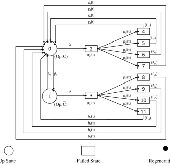
3. State Transition Diagram

1

0 2

3

4

5

6

7

8

9

10

11 h4(t)

h3(t)

h2(t)

h1(t) g4(t)

g3(t)

g2(t)

g1(t)

λ

λ β1

β2

) C , Op (

) C , Op

( (Fi,C)

) C , F (i

(Fr1)

(Fr2)

(Fr3)

(Fr4)

(Fr1)

(Fr2)

(Fr3)

(Fr4) p1i(t)

p2i(t)

p3i(t)

p4i(t)

p1i(t)

p2i(t)

p3i(t)

p4i(t)

Up State Failed State Regenerative Point

(4)

4. Model Description and Assumptions

1) Initially the system is operative with controlled power factor.

2) Then it may transit to state where power factor is not controlled.

3) There are four types of failure: Fuse blown off, Transformer burnt, Programming problem, Output relay faulty.

4) Inspection is carried out to detect the type of failure. The system undergoes inspection irrespective of the power factor is controlled or not.

5) Failure times are assumed to follow an exponential distribution, whereas the other times follow arbitrary distributions.

6) After repair, the system becomes operative with controlled power factor.

5. Transition Probabilities and Mean Sojourn Times

The transition diagram showing various states of transition of system are shown in Fig. 1. The epochs of entry into the states 0,1,2,3,4,5,6,7,8,9,10 and 11 are regenerative points and therefore these states are regenerative states. The transition probabilities from regenerative state to regenerative state are given below:

dQ01(t) =



₁

_e

(1)t_{dt dQ40(t) =}

_g

₍

_t

₎

1 dt

dQ02(t) =



e

(1)t_{dt dQ50(t) =}

g

(

t

)

2 dt

dQ10(t) =



₂

_e

(2)t_{dt dQ60(t) =}

_g

₍

_t

₎

3 dt

dQ13(t) =



e

(2)t_{dt dQ70(t) =}

g

0 slim ij

q(s) such that

01

p + p₀₂ = 1 p10 + p13 = 1

24

p +

p

25 +

p

26 +

p

27 = 1 p38 +p39 +p3,10+ p3,11= 1

40

p = p50=p60=p70=1 p80 =p90=p10,0=p11,0= 1

The mean sojourn times (i) in the regenerative state i is defined as the time of stay in that state before transition to any other state. If T denotes the sojourn time in the regenerative state i, then;

i = E (T) = Pr(T>y)

0 =

1

 

 , 1 = ₂

1

 



0

4(t)dt

tg

m24 + m25 +m26 + m27 = 2 m80 = 8 m38 + m39 +m3,10 + m3,11 = 3 m90 = 9 m40 = 4 m10,0 = 10 m50 = 5 m11,0 = 11

6. Calculations of Measures of System Effectiveness

Considering the failed states as absorbing states and using the probabilistic arguments used for regenerative processes, we obtained the recursive relations for mean time to system failure (MTSF), availability when power factor is controlled, availability when power factor is not controlled, busy periods for repair of type I, type II, type III and type IV failure, expected number of visits of the repairman, expected number of fuse replacements, expected number of transformer replacement. Then employing Laplace/ Laplace Stieltj’s Transforms of these recursive relations, the steady-state solutions for the above mentioned measures of system effectiveness are obtained as under:

Mean Time to System Failure (MTSF) = N/D Availability when power factor controlled (AC0) = N1/D1 Availability when power factor not controlled (AC₀) = N2/D1 Busy Period of Type I Repair (BF0) = N3/D1 Busy Period of Type II Repair (BT0) = N4/D1 Busy Period of Type III Repair (BP0) = N5/D1 Busy Period of Type IV Repair (BO0) = N6/D1 Expected Number of Visits of the Repairman (V0) = N7/D1 Expected Number of Fuse Replacements (FR0) = N8/D1 Expected Number of Transformer Replacements (TR0) = N9/D1 where

N = ₀+ p₀₁₁ D = 1- p₀₁ p₁₀

D1=₀+p₀₁1+p02 2+p01p133+p02p24 4 +p02p25 5+p02p26 6+p02p27 7+p01p13p388

+p01p13p399 + p01p13p3,1010 + p01p13p3,1111 N1 = ₀

N2 = ₁p₀₁

N3 = (p02p24p01p13p38) 4

N4 = (p₀₂p₂₅p₀₁p₁₃p₃₉) ₅ N5 = (p₀₂p₂₆p₀₁p₁₃p₃_,₁₀)₆ N6 = (p₀₂p₂₇p₀₁p₁₃p₃_,₁₁) ₇ N7 = p₀₂ p₀₁p₁₃

N8 = p₀₂p₂₄+p₀₁p₁₃p₃₈ N9 = p₀₂p₂₅+p₀₁p₁₃p₃₉

7. Profit Analysis

In steady state, the expected profit per unit time incurred to the system is given by:

) t (

i = et, g₁(t)= ₁_e1t_,_g ₍_t₎

2 = 2e2t , g3(t)= 3e3t , g4(t)= 4e4t

1

h (t)= 1t

1e

 , h (t)₂ = 2t

2e

 , h (t)₃ = 3t

3e

 , h (t)₄ = 4t

4e



(6)

C1=50, C2= 250, C3=1000, C21=100, C22= 150, C23= 50, C24= 75,

L

C

= 500) the following values of various measures of system effectiveness are obtained:

1) Mean Time To System Failure (MTSF) = 999.999 Hours

2) Availability when Power Factor is Maintained as per Requirement (AC0 ) = 0.909104

3) Availability when Power Factor is not Maintained as per Requirement (

A

C

₀ ) = 0.090458 4) Busy period of Type I repair (BF0) = 0.000075

5) Busy period of Type II repair (BT0) = 0.0001 6) Busy period of Type III repair (BP0) = 0.000067 7) Busy period of Type IV repair (BO0)= 0.00001

8) Expected number of Visits of the repairman (V₀)= 0.001 9) Expected number of Fuse Replacement (FR₀) = 0.0003 10) Expected number of Transformer Replacement (TR₀) = 0.0002

11) Profit incurred to the system (P) = 953.24225

9. Graphical Interpretation

From the data/information gathered for various estimates of rates, costs and probabilities are obtained and hence the various measures of system effectiveness like mean time to system failure, availability when power factor controlled, availability when power factor not controlled, and profit are calculated for different values of failure rate. It was observed that mean time to system failure decrease with increase in the values of failure rate. Similarly, availability (when power factor controlled), availability (when power factor not controlled) and profit decrease with the increase in failure rate.

Various graphs have been plotted; some of them have been shown in Figs. 2 to 4. To avoid repetition of similar interpretation, other graphs have not been shown. However, the readers of the paper and users of such systems may plot many other graphs as per their requirement and on the basis of the data available to them in taking very important decisions regarding profitability of the system. However, the graphs shown and their interpretations are given as under:

-100 -50 0 50 100 150

350 370 390 410 430 450 470 490 510 530

PR

O

FI

T

(

P)

β1=0.7 β1=0.74 β1=0.78

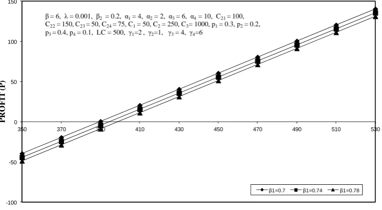
β = 6, λ = 0.001, β2= 0.2, α1 = 4, α2= 2, α3= 6, α4= 10, C21 = 100, C22= 150, C23 = 50, C24 = 75, C1= 50, C2= 250, C3= 1000, p1= 0.3, p2= 0.2, p3 = 0.4, p4= 0.1, LC = 500, γ1=2 , γ2=1, γ3= 4, γ4=6

REVENUE PER UNIT UP TIME (C0)

Fig. 2. Profit (P) versus revenue per unit up time with (C₀) for different values of the rate with which power factor changes from

controlled mode to uncontrolled mode (β1)

(7)

-850 -750 -650 -550 -450 -350 -250 -150 -50 50 150 250 350 450 550

1200 1400 1600 1800 2000 2200 2400

PR

O

FI

T

(

P)

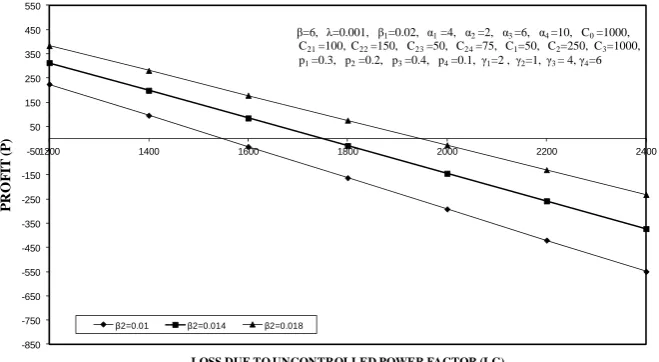
LOSS DUE TO UNCONTROLLED POWER FACTOR (LC) β2=0.01 β2=0.014 β2=0.018

β=6, λ=0.001, β1=0.02, α1=4, α2 =2, α3 =6, α4 =10, C0=1000,

C21=100, C22=150, C23=50, C24=75, C1=50, C2=250, C3=1000,

p1=0.3, p2=0.2, p3=0.4, p4=0.1, γ1=2 , γ2=1, γ3 = 4, γ4=6

Fig. 3. Profit (P) versus loss due to uncontrolled power factor (LC) for different values of the rate with which power factor changes from

uncontrolled mode to controlled mode (β2)

Fig. 3 reveals the behavior of profit (P) with respect to loss ( CL ) due to uncontrolled power factor for different values of the rate with which power factor changes from uncontrolled mode to controlled mode (β2). It can be concluded that the profit decreases with the increase in the value of CL and has higher values for higher rates of β2. It can also be noticed that if β2 = 0.01 then P < or = or > 0 accordingly as CL > or = or < 1550. So, for the model to be beneficial for β2 = 0.01, CL should be < 1550. Similarly, for β2 = 0.014 and β2 = 0.018, the values of CL should be less than 1750 and 1950 respectively.

-0.8 -0.6 -0.4 -0.2 0 0.2 0.4 0.6 0.8

550 1050 1550 2050 2550 3050 3550 4050

PR

O

F

IT

(

P)

COST PER FUSE REPLACEMENT (C1)

C3=1000 C3=1040 C3=1080

β = 6, β1= 0.02, β2 = 0.2, α1 = 4, α2= 2, α3= 6, α4= 10, C0= 200,

C21= 100, C22= 150, C23= 50, C24= 75, C2= 250, p1= 0.3, p2= 0.2,

p3= 0.4, p4= 0.1, λ = 0.001, LC = 500, γ1=2 , γ2=1, γ3= 4, γ4=6

Fig. 4. Profit (P) versus cost per fuse replacement (C1) for different values of cost per visit of repairman (C3)

Fig. 4 depicts the behavior of profit (P) with respect to cost per fuse replacement (C1) for different values of cost per visit of repairman (C3). It is obvious from the graph that the profit decreases with the increase in the value of cost per fuse replacement (C1). It can also be noticed that if C3 =1000 then P < or = or > 0 accordingly as C1 > or = or < 2500. So, for the model to be beneficial for C3 = 1000, the C1 should be < 2500. Similarly, for C3 = 1040 and C3 = 1080, the value of cost per fuse replacement (C1) should be less than 2200 and 2175 respectively.

Similarly, the behavior of profit (P) with respect to cost per transformer replacement (C2) for different values of cost per visit of repairman (C3) may be plotted and interpreted accordingly.

(8)

References

[1] Charles E. Ebeling, “Reliability and Maintainability Engineering” Tata McGraw-Hill, 2000, pp. 398-400.

[2] Goel, L. R., Sharma, G. C. and Gupta, Parveen “Stochastic behavior and profit analysis of a redundant system with slow switching

device”, Microelectron. Relab, 26, 215-219, 1986.

[3] Gopalan, M. N. and Bhanu, K.S. “Cost analysis of a two unit repairable system subject to on line preventive maintenance and/or

repair.”, Microelectron. Relab, 35(2), 251-258. 1995.

[4] Khurana, Vipin, Rizwan, S.M. and Taneja, G. “Modeling and optimization of single unit PLCs' system” International Journal of

Modeling and Simulation, 27(4), 361-368, 2007.

[5] Mathew A.G., Rizwan SM, Majumdar MC, Ramachandran KP & Taneja G, Profit evaluation of a single unit CC plant with scheduled

maintenance , Caledonian Journal of Engineering, 2009; 5:1-5.

[6] Mokaddis, G.S., Tawfek, M.L. And Elhssia, S.A.M., “Cost analysis of two dissimilar unit cold standby redundant system subject to

inspection and two types of repair”, Microelectron. Relab, 37(2), 329-334, 1997.

[7] Murari K & Maruthachalan C, The reliability of a two-unit system with two different interlinkings in two different periods, J opl Res

Soc , 1984; 35: 835-845.

[8] Parashar, Bhupender and Taneja, G. , “Reliability and profit evaluation of a PLC hot standby system based on master slave concept

and two types of repair facilities. “ IEEE Transactions on Reliability, 56(3), 534-539, 2007.

[9] Singh, D.V., Minocha, Amit and Taneja, G.” Profit analysis of 2-out-of-3 unit system for an ash handling plant wherein situation of

system failure did not arise.” Journal of Information and Optimization Sciences, 28(2), 195-204, 2007.