ARTIFICIAL NEURAL NETWORK TO
PREDICT RESONANT FREQUENCY OF
DIPOLE FREQUENCY SELECTIVE
SURFACE
POULAMI SAMADDAR*, NURNIHAR BEGAM, DEBASREE CHANDA SARKAR AND PARTHA PRATIM SARKAR
Department of Engineering and Technological Studies, University of Kalyani, Kalyani, West Bengal, 741235, India
[email protected], [email protected], [email protected], [email protected]
Abstract: This paper deals with a frequency selective structure comprising of two dimensional arrays of dipole patches. The characteristics of Frequency Selective Surface can be calculated by Finite Element Method, Method of Moment etc. But these methods are very complicated and time consuming. Efforts have been given to develop a method which may relate the resonant frequency with the periodicities and dielectric constant of an FSS having dipole patches. Firstly resonant frequencies for each of the combinations have been calculated using Method of Moment after selecting proper basis function. Some of the resonant frequencies obtained have also been compared with the measured results for validation. These results have been used to train an artificial neural network. From the trained network resonant frequencies for given periodicities and dielectric constant may be readily available. It is observed that the results obtained by the trained artificial neural network are very fast and accurate.
Keywords: Frequency selective structure (FSS); artificial neural network (ANN); resonant frequency; Dipole;
Patch.
1. Introduction
Frequency selective surface (FSS) is a two dimensional array of patch type or aperture type element. Depending on the element type, this device shows band pass or band stop property [1]. This filtering property is very interesting feature of these structures. Recently FSS is used in different fields like radar systems, telecommunication, military and wireless security etc [1, 2]. The array of elements is mainly supported by a dielectric substrate. The center frequency (resonant frequency) of these structures depends on many factors like the dielectric constant of the substrate, the structure of the patch or the aperture type element, the periodicity of the array elements etc [1-5]. To know the frequency response of FSS some mathematical tools like Finite Element Method (FEM), Method of Moment (MoM), Finite Difference Time Domain (FDTD) etc. can be used. The characteristics curve can be calculated by some commercially available software like ansoft designer nexxim, CST, FEKO, IE3D etc. which use these mathematical tools. But this process is very time consuming and requires very high computational power and the software products are very costly. In many cases the time taken to simulate a simple design (like dipole, square, circle etc.) is more than one hour depending on the computer configuration.
2. Frequency Selective Surface
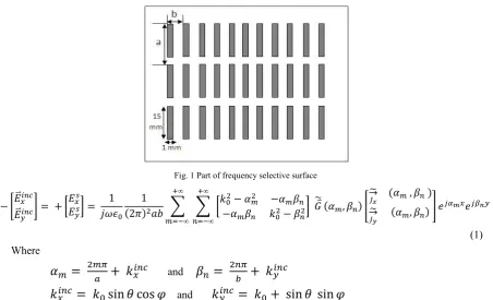
Typically a frequency selective surface consists of one or more metallic patch supported by one layer or multiple layers of dielectrics. According to transmission property there are mainly two types of FSS, one is stop band (patch type) and another is pass band (aperture type) [1-5]. This paper deals with dipole patch type FSS which acts like a band stop filter. Dipole type patches with length and width 15 mm and 1mm respectively are designed here. The training set is generated by changing the periodicity (in x or y direction) and dielectric constant (ε) of the dipole patch. The other parameters (like patch dimension etc.) are kept same. The periodicity in x and y direction is ‘a’ (varied from 5 mm to 14 mm) and ‘b’ (varied from 19 mm to 30 mm) as shown in Figure 1.
The transmission coefficient can be calculated by MoM (Method of Moment), which has been described below in brief. From incident electric field current density may be calculated by the following equation which is derived from reference [15].
Fig. 1 Part of frequency selective surface
1 1
2
∞
∞
,
→ ,
→ ,
∞
∞
(1) Where
and
sin cos
andsin sin
Where θ is the angle of incident wave with the z-axis on xz plane and φ is the angle of the projection of the incident wave on the xy plane with the x-axis, ‘a’ and ‘b’ is periodicity in x and y direction respectively. Skew angel is taken as zero.
For solution, the matrix equation is represented by
L(u) = g where g is known matrix
→
→
And u in the matrix to be determined
→
α , β
→
α , β
and L is the total operators involved in previous matrix equation 1.
For dipole aperture or patch type frequency selective surface the basic function may be considered as [4]
sin
0,
(2)Where p = 0, 1, 2… and L = Length of the dipole
After taking Fourier transform of equation 2 we can get the values of matrix
→ ,
→ , .
Now using these values of → and → into equation (1) we can calculate scattered electric fields .
From these scattered electric field ; the transmission coefficients of the structure of mode mn due to mode kl incident is given by [5]
Where
Or =
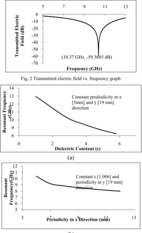
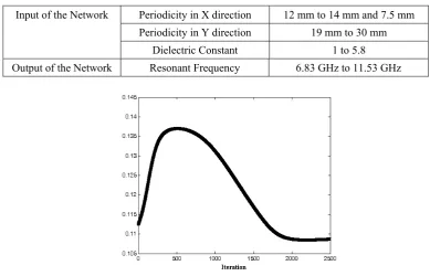
Ansoft designer software uses this method to calculate transmission electric field vs. frequency graph for a particular frequency selective structure. From that graph we can get the resonant frequency (fr) as shown in figure 2. To generate the training and validation set for ANN, different resonant frequencies for different FSS designs have been simulated and noted. For this paper 560 simulations have been done. The resonant frequency calculated for 6 GHz to 12 GHz. Figure 3 shows the relation between resonant frequencies with different changing parameters. To validate the simulated result some fabrication is done. Practically measured data showed good parity with simulated one.
Fig. 2 Transmitted electric field vs. frequency graph
(a) (b) -70 -60 -50 -40 -30 -20 -10 0
5 7 9 11 13
Transm
itted Electric
Field (dB)
Frequency (GHz)
(10.37 GHz, -59.3685 dB)
8 9 10 11 12 13 14
0 2 4 6
Resonant Frequency
(GHz)
Dielectric Constant (ε)
Constant prediodicity in x [5mm] and y [19 mm] direction 5 6 7 8 9 10 11 12
5 7 9 11 13
Resonant
Frequency(GHz
)
Periodicity in x Direction (mm)
Fig. 3 Change of resonant frequency with (a) dielectric constant (ε), (b) periodicity in x direction and (c) periodicity in y direction
3. Artificial Neural Network
Artificial neural networks are successfully applied to solve many real world problems, which are very hard to track by expert systems. These networks can predict the relationship between the input and output set without any knowledge of the model. For this property it can solve the problems related with complex engineering systems, difficult electromagnetic computation etc. Multilayered neural network can be trained with different algorithms. These networks have mainly three layers i.e. input, hidden and output layer. These are connected by weighted synapse. At first an output is calculated by the network for a known input output set. The output generates an error with respect to the original output. The error is then propagates backward and changes the weight values. This process is called training and weight values after the training is called trained weight. This training process continues until the error decreases to a certain range which is set by the programmer [5-14]. In this paper a multilayered feed forward back propagation network is used to predict the resonating frequency. This network uses gradient descent algorithm to minimize the error. Gradient decent method is a very stable method and is tested satisfactorily for several years [5, 6]. Levenberg-Marquardt method is also used to train the network. This network has three input neuron (change of periodicity in x and y direction and dielectric constant) in input layer, one output neuron (resonant frequency) in output layer. Detailed profile for 450 input data is shown in table 1. The three input variables are independent variable. The input-output data set is normalized before it is applied to train the network. Normalization is done after dividing each of them by maximum value of the data set.
Fig. 4 Neural Network Structure Table 1. Tanning data used to train Neural Network
Input of the Network Periodicity in X direction 5 mm to 12 mm Periodicity in Y direction 19 mm to 30 mm Dielectric Constant 1 to 5.8
Output of the Network Resonant Frequency 6.2 GHz to 12 GHz
Different network topologies are used to achieve the optimized one. First one hidden layer with seven nodes and two layers with five-three neuron is used. But best result obtained by three hidden layers which have seven-fifteen-seven neuron formation. Learning factor (η) is kept 0.5. Fig. 4 shows the network. Total 450 data (80%
9 9.5 10 10.5 11
15 20 25 30 35
Resonant
Frequency(GHz
)
Periodicity in y Direction (mm)
4. Result and Discussion
Some of the simulated results by Ansoft software have been verified with the practically fabricated structures for validation of the simulation process. Table 2 shows that comparison of simulated and practically measured data. It can be observed that the results are in good parity. Measurement is done by standard microwave test bench.
Table 2 Comparison between Measured and ANN results
Input (periodicity in x and y direction [mm] and dielectric constant )
Measured Resonant
Frequency [GHz] Simulated Resonant frequency [GHz] Absolute % Error
12, 25, 2.8 7.9 8.11 0.21 2.66%
12, 26, 2.8 8.1 8.11 0.01 0.1%
12, 30, 2.8 8.2 8.05 0.0502 1.8%
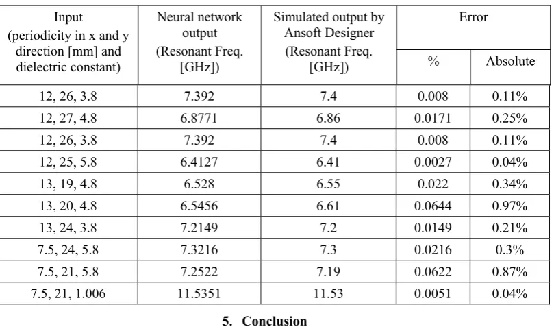
Neural networks which have different numbers of hidden layers are trained with the same 450 training data. One hidden layer network and two hidden layer network show less error minimization than three layers. The error minimization with iteration plot for two hidden layer ANN using gradient decent is shown in figure 5. The lowest error is achieved by three hidden layer network. Figure 6 and figure 7 shows error minimization plot for three hidden layer LM method and gradient decent method respectively. It can be observed that although LM method converge very fast but for this data set the gradient descent method provide very small error at the time of training than Levenberg-Marquardt. After training, the r.m.s. error became 0.000001 using three hidden layer with gradient decent method. Some random values (about 115) are tested with this trained network. Train to test data split ratio is kept 80%. Table 3 shows the range of test input-output data. Some of them with simulated resonant frequency, ANN output, and absolute, percentage error are shown in table 4. It is observed that the test results are satisfactory for all the cases.
Table 3. Test data used to validate trained Neural Network
Input of the Network Periodicity in X direction 12 mm to 14 mm and 7.5 mm Periodicity in Y direction 19 mm to 30 mm
Dielectric Constant 1 to 5.8 Output of the Network Resonant Frequency 6.83 GHz to 11.53 GHz
Fig. 6 Error minimization with iteration for three hidden layer ANN using Lavenberg-Marquardt method
Fig. 7 Error minimization with iteration for three hidden layer ANN using gradient decent method Table 4. Comparison between ANN and Simulated results
Input
(periodicity in x and y direction [mm] and dielectric constant)
Neural network output (Resonant Freq.
[GHz])
Simulated output by Ansoft Designer (Resonant Freq.
[GHz])
Error
% Absolute
12, 26, 3.8 7.392 7.4 0.008 0.11%
12, 27, 4.8 6.8771 6.86 0.0171 0.25%
12, 26, 3.8 7.392 7.4 0.008 0.11%
12, 25, 5.8 6.4127 6.41 0.0027 0.04%
13, 19, 4.8 6.528 6.55 0.022 0.34%
13, 20, 4.8 6.5456 6.61 0.0644 0.97%
13, 24, 3.8 7.2149 7.2 0.0149 0.21%
7.5, 24, 5.8 7.3216 7.3 0.0216 0.3%
7.5, 21, 5.8 7.2522 7.19 0.0622 0.87%
7.5, 21, 1.006 11.5351 11.53 0.0051 0.04%
5. Conclusion
References
[1] Munk, B.A. (2000). Frequency selective surfaces: theory and design. New York: Wiley-Interscience Publication.
[2] Zhou, H. Qu, S.-B. Wang, J.-F. Lin, B.-Q. Ma, H. Z. Xu, Bai and Peng, P. W.-D. (2012). Ultra-wideband frequency selective surface. Electronics Letters. 48(1), pp. 11-13.
[3] Sarkar, D. Sarkar, P.P. and Chowdhury, S. K. (2004). Experimental Investigation of A Tri-Band Frequency-Selective Surface. Microwave and Optical Technology Letters. 41(6), pp. 511-512.
[4] Barchloui, N.K. and Solaimani, M. (2004). Simulation of Frequency Selective Surface Using 3D Transmission Line Matrix Method. Iranian Journal of Science & Technology, Transaction B., 28 (B3), pp. 359-364.
[5] Samaddar, P. Nandi, S. Nandy, S. Sarkar, D.C. and Sarkar, P. P. (2014). Prediction of resonant frequency of a circular patch frequency selective structure using artificial neural network. Indian Journal of Physics, 88 (4), pp. 397-403.
[6] da Silva, M. R. Nobrega, C. de L. Silva, P. H. da F. and D’Assuncao, A. G. (2014). Optimization of FSS with Sierpinski Island Fractal Elements Using Population-Based Search Algorithms And MLP Neural Network. Microwave and Optical Technology Letters. 56 (4), pp. 827-831.
[7] Panda, M. Nandi S. and Sarkar, P. P. (2015). A comparative study of performance of different back-propagation neural network methods for prediction of resonant frequency of a slot-loaded double-layer frequency-selective surface. Indian Journal of Physics. 89 (12), pp. 1283–1286.
[8] Ferreira, D. Caldeirinha, R. F. S. Cuiñas, I. and Fernandes. T. R. (2015). Square Loop and Slot Frequency Selective Surfaces Study for Equivalent Circuit Model Optimization. IEEE Transactions on Antennas and Propagation. 63 (9), pp. 3947-3955.
[9] Attar, A.R. Sheikhi, A. Abiri, H. and Mallahzadeh. A. (2006). A New Method for Communication System Recognition. Iranian Journal of Science & Technology, Transaction B, Engineering. 30 (B6), pp. 775-788.
[10] Ezema, L. S. and Ani, C. I. (2017). Artificial Neural Network Approach to Mobile Location Estimation in GSM Network. Intl Journal of Electronics and Telecommunications. 63(1), pp. 39-44, 2017.
[11] Gangwar, S. P. Gangwar, R.P.S. Kanaujia, B. K. and Paras. (2008). Resonant frequency of circular microstrip antenna using artificial neural networks. Indian Journal of Radio & Space Physics. 37 (3), pp. 204-208.
[12] Singh, J. Singh, A. P. Kamal, T. S. (2012). Estimation of Resonant Frequency of a Circular microstrip Antenna Using Artificial Neural Network.. J. Inst. Eng. India Ser. B. 93(1), pp. 7-13.
[13] Ayestarán, R. G. Las-Heras, F. and Martínez, J. A. (2007). Non Uniform-Antenna Array Synthesis Using Neural Networks. J. of Electromagn. Waves and Appl. 21(2), pp. 1001-1011.
[14] Habibzadeh-Sharif, A. Yamini, A. H. and Soleimani, M. 2007. Accurate Analysis and Design of Circularly Polarized Dual-Feed Microstrip Array Antenna Using Multiport Network Model. Iranian Journal of Science & Technology, Transaction B, Engineering. 31 (B3), pp. 377-384.