---ABSTRACT---
The associative memory feature of the Hopfield type recurrent neural network is used for the pattern storage and pattern authentication. This paper outlines an optimization relaxation approach for signature verification based on the Hopfield neural network (HNN) which is a recurrent network. The standard sample signature of the customer is cross matched with the one supplied on the Cheque. The difference percentage is obtained by calculating the different pixels in both the images. The network topology is built so that each pixel in the difference image is a neuron in the network. Each neuron is categorized by its states, which in turn signifies that if the particular pixel is changed. The network converges to unwavering condition based on the energy function which is derived in experiments. The Hopfield’s model allows each node to take on two binary state values (changed/unchanged) for each pixel. The performance of the proposed technique is evaluated by applying it in various binary and gray scale images. This paper contributes in finding an automated scheme for verification of authentic signature on bank Cheques. The derived energy function allows a trade-off between the influence of its neighborhood and its own criterion. This device is able to recall as well as complete partially specified inputs. The network is trained via a storage prescription that forces stable states to correspond to (local) minima of a network “energy” function.
Keywords: Hopfield Neural Network, Pattern Matching, Signature Verification.
--- Paper submitted: 02.04.2009 Accepted: 10.06.2009
---
1.INTRODUCTION
wo decades ago, most banks reviewed nearly 100% of the signatures of cheque makers when they paid and manually filed cheques in file drawers in the branch. As banks grew in size and as the number of accounts, customers, and cheques processed dramatically increased, the need grew for more controlled, reliable, and efficient methods for processing and paying cheques. Accordingly, cheque storage was centralized and automated in large processing centers where the signatures of some, but not all, items were compared with the signatures on a signature card, a microfilm copy of the signature card, or a stored digital
image of the signature card. With the move of the cheque pay-and-file process from the branches into large processing centers and the increase in cheque volume, signature verification changed from review of all signatures to a review of a portion of the signatures – usually large amount transactions, accounts with special arrangement to cheque multiple signatures, and a random sampling of all cheques, regardless of amount.
Handwritten signature verification has been extensively studied in this decade. Its many applications include cheques, credit card validation, security systems, certificates, contracts, etc. Comparing signature verification with fingerprint, face, voice and other recognition technologies
Enhancing the Authentication of Bank Cheque
Signatures by Implementing Automated System
Using Recurrent Neural Network
Mukta Rao
Kanya Gurukul Mahavidyalaya, Gurukul Kangri Vishwavidyalaya, Dehradun Email: [email protected]
Nipur
Kanya Gurukul Mahavidyalaya, Gurukul Kangri Vishwavidyalaya, Dehradun Email: [email protected]
Vijaypal Singh Dhaka
Department of Computer Science, MSIT, New Delhi Email: [email protected]
such as retina and iris scanning, signature verification has several advantages as an identity verification mechanism:
• The capture of signature has the untouchable merits and very easy to be social accepted.
• Signature analysis can only be applied when the person is/was conscious and -disposed to write in the usual manner, although they may be under extortion to provide the handwriting [1].
• Forging a signature seems to be more difficult than a fingerprint given the availability of sophisticated analyses
However, for several reasons the task of verifying human signatures cannot be considered a trivial pattern recognition problem. It is a more difficult problem because signature samples from the same person are similar but not identical. In addition, a person's signature often changes radically during their lifetime. In fact great variability can be observed in signatures according to country, age, time, habits, psychological or mental state, physical and practical conditions [2].
There are two major methods of signature verification. One is an on-line method to measure the sequential data such as handwriting and pen pressure with a special device. The other is an off-line method that uses an optical scanner to obtain handwriting data written on paper. Handwriting recognition in off-line systems is more difficult than in on-line systems as a lot of dynamic information is lost. Hence, on -line signature verification is generally more successful. Nevertheless, off-line systems have a significant advantage in that they do not require access to special processing devices when the signatures are produced.
In fact, if the accuracy of verification could be promoted greatly, the off-line method has much more practical application areas than that of the on-line one. The process of off-line signature verification often consists of a learning stage and a testing stage. The purpose of the former is to create a reference file, and that of the latter is to compute the similarities between the testing and its corresponding reference signature to check whether the tested signature is genuine.
When we verify a signature is genuine or not, there are two types of errors: False Rejection, which is also called Type I errors; and False Acceptance, which is also called Type 2 errors. Also, there are two types of rates: False Rejection Rate (FRR) which is the percentage of genuine signatures rejected as false; and False Acceptance Rate (FAR) which is the percentage of false signatures accepted as genuine. When discussing the experiments, the results are reported in terms of FRR and FAR. But if we try to lower the FAR too much then FRR will increase. We do then have a trade off between these two types of errors and depending on the application and other aspects of where and how the system is used. We will need to optimize it in different ways.
Signature is a ballistic movement, has some characteristics such as, it is user-friendly, non invasive, as a pattern it is stored in number of applications, it is ubiquitous, it can be changed on a compromise, it is not dependent on age [3] and it is well exposed to forensic environments .The design of an accurate algorithm for verification is still an open problem [4]. Some of the different types of signatures are simple, cursive, graphical [5] and not a connected curve pattern
(Chinese signatures [6]). In off-line method, the signatures are treated as grey level images. The image can be scanned from a copy of document [7] or can be a saved file acquired by a tablet in a keyboard-less user interface.
Various methodologies have been used by researchers over the time to verify the signatures. Warping based matching methods produce the order of the coordinates and are able to match the coordinates that are placed in the same position in the two exterior curves that are formed by top and bottom parts of the template signature as test signature [8, 9].
The other effective graph matching approach is proposed by using deformable templates based on multi-resolution shape features [10]. Hidden Markov Models has ability to absorb both variability and the similarity between patterns in the problems that have an inherent temporality [11]. Forward algorithm of HMM is also used to determine the verification probability [12, 13, and 14]. Using modified direction and transition distance feature (MDF) structural features can be extracted from the signature’s contour [15]. The other approaches are human centric method [16], wavelet based methods, Pseudo bacterial genetic algorithm methods(PBGA) [5] , statistical methods [17 , 18, 19] , Neural network based methods [20, 21, 22] and hybrid method [23]. Shape analysis techniques based on spatial transforms include Principal component analysis (PCA), Fisher discriminate analysis and Fast Fourier transform which extract the numerical values of features for classification.
The pseudo-dynamic features are used to detect skilled forgeries, because it is possible to recover pressure information from the image of the signature using the pseudo-dynamic features [24].
Signatures are symbols, which are usually cursively written and graphical in appearance. It is often difficult, even for humans at instances, to segment the signature images into letters or basic lexical constructs, and to recover the underlying handwriting sequence. The common approaches to off-line signature verification have been to exploit the static features of the handwriting, treating the complete signature as a single entity.
As we have discussed so far that signature verification techniques have used quite many types of Artificial Neural networks such as Multi-Layer Perceptron, Radial Basis Function Networks, Hidden Markov Models, Support Vector Machines etc. But we also have another type of very efficient and fast ANN i.e. Hopfield neural network. This network although works in unsupervised way and best suited for pattern recalling applications, but we can use its excellent feature of energy minimization for Signature verification as well.
In this paper we are proposing as network architecture for automated verification of signatures based on Hopfield neural network. The proposed network work on the idea of image change detection percentage. We enforce the network to learn the signature patterns and then recall them to compare with test sample signatures. In the following material we are presenting the quick introduction and advancements in the usage of Hopfield Neural Network.
definition of “energy” in the net and a proof that the net operated by minimizing this energy when settling into suitable patterns of operation [26], this helped to reignite the dormant world of Neural Networks once again. This network has attracted considerable interest both as a content address memory (CAM) and, more interestingly, as a method of solving difficult optimization problems [27-29]. The focus for solving optimization problems for researchers have been Hopfield network because of the advantages such as massive parallelism, convenient hardware implementation of the neural network architecture, fully interconnected and a common approach for solving various optimization problems [30].
Hopfield proposed two types of neural networks; Discrete Hopfield Network (DHN) and Continuous Hopfield Network(CHN). Those have been used for solving the famous travelling salesman problem in a sense of optimization [39]. DHN, a stochastic model is simple to implement and fast in computing, but it uses binary value for states of neurons resulting in an approximate solution. On the other hand, CHN gives a near-optimal solution. However, it takes too much time to simulate a differential equation which provides a main characteristic of CHN. A matching problem using a graph matching technique can be cast into an optimization problem [28].
It has been proven by Hopfield that the network converges when the weights are symmetric with zero diagonal elements (i.e. wij = wji & wii = 0) for the hard limiting nonlinear neuron [25]. This stands true when monotonic “sigmoid” neurons with the zero diagonal elements are included in the energy function [26]. Some researchers have studied the possessions of the Hopfield neural networks with zero diagonal elements in the area of combinatorial optimization problems [31]. The experiments conducted were based on a binary Hopfield neural network with a negative self-feedback on same problem domain. An oscillatory neuron unit was also proposed by adding a simple self-feedback, which could also be negative or positive along with an energy value extraction circuit [32-33]. However, each of them attempts to make some local minima unstable by introducing a negative self-feedback or using an oscillatory neuron.
Some researchers apply the Continuous Hopfield Network to three-dimensional object matching problem [34]. However, Continuous Hopfield Network takes much computational time in simulating a differential equation even though it provides good solutions. The Discrete type Hopfield Network has been used for two-dimensional objects matching problems [35]. However, DHN is an approximation method and gives only rough solutions, but it reduces computational time. Unlike the travelling salesman problem implemented by the Hopfield neural network [40, 41], the matching problem is handled by normalizing features made by a fuzzy function which gives distinguishable values to a connectivity matrix.
The proposed network architecture in this paper is DHN (Discrete Hopfield Network). The DHN learn the sample signature from the cheque leaves in unsupervised way, but the recalling of the same for test samples has been carried by applying constraint of threshold. The difference image is used to judge the authentication.
The rest of the paper is organized as follows. Section 2 provides a brief description of the Hopfield model as well as some terminologies to be used throughout the paper. Section 3 explains the implementation procedure. Section 4 details the pre-processing, training & test signature samples. Section 5 describes the experimental results. Finally, Section 6 concludes the paper followed by references.
2.TECHNICAL ASPECTS OF HOPFIELD NEURAL NETWORK
Recurrent networks are networks those have closed loops in the network topology. In this paper, a form of recurrent neural network suitable for auto associative (content) addressable memory and its characteristics, optimization and constraint satisfaction application is considered. This network is often referred to as Hopfield network in the honor of John Hopfield. The topology is very simple: it has ‘n’ neurons, which are all networked with each other or fully interconnected. The net has symmetric weights with no self connections i.e. all the diagonal elements of the weight matrix of Hopfield net are zero.
The two main differences between Hopfield and iterative auto associative net (recurrent associative net) are that, in the Hopfield net.
• Only one unit updates its activation at a time, and, • Each unit continues to receive an external signal in
addition to the signal from the other units in the net. The following sections will detail all steps in the formulation and design of this proposed recurrent network and its functional details.
2.1 Architecture and Mathematical Foundation of Hopfield Network
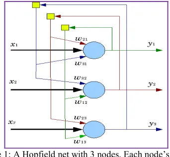
The proposed system’s architecture is shown in figure 1. This Hopfield network consists of a set of neurons and a corresponding set of unit delays, forming a multiple loop feedback system. A feed-back system is the one, whose output is the number of feed-back loops is equal to the number of neurons.
Figure 1: A Hopfield net with 3 nodes. Each node’s output is fed-back to all other nodes.
The learning of signature samples is based on the energy convergence principal of Hopfield Neural Networks. The computation of HNN’s energy and its dependence is discussed in this section and a pathway to energy minima is also suggested.
Hopfield network considered here is made up of neurons which possess additive model (current summing model). We know from the rule of energy convergence and voltage stability that each network follows the rules given by Kirchoff. From Kirchoff’scurrent low, on the input node of the HNN, which has N number of neurons and at a particular time t, we get the equation for the HNN state as:-
c
j dt t dvj()= - j j
R
t
v
(
)
+
∑
= N i i jix
t
w
1
)
(
+ Ij, For all j = 1, 2, ….., N (2.1)
Where j
R
= leakage resistance
)
(
t
x
i= stimuli acting on synaptic weights. ji
w
= synaptic weight.
)
(
t
v
j= induced local field at the input
c
j = leakage capacitance Ij= current source/ externally applied biasRecognizing that
x
i(
t
)
= ф()
(
t
v
j)
c
j = -dt
d
vj(t) =
j j
R
t
v
(
)
+
∑
= N i i i jiv
t
w
1))
(
(
ϕ
+ Ij ,
j = 1, 2, ….., N (2.2) Where ф (vj(t)) is the non-linear activation function.
This dynamic has got following assumptions:-
1. The matrix of synaptic weights is symmetric: wji = wij for all i and j
2. Each neuron has a non linear activation of its own – hence ф (vj(t)) used in equation.
3. The inverse of the nonlinear activation function exists, so we may write:-
)
(
1
x
v
=
ϕ
i− (2.3)Let the sigmoid function ф (vj(t)) be defined by the
hyperbolic tangent function
) exp( 1 ) exp( 1 2 tanh ) ( v a v a v a v x i i i
i + −
− − = = =
ϕ
(2.4) Which has the slope of ai/2 at the origin as shown by -0
2
=
v=i i
dv
d
a
ϕ
(2.5) Henceforth we refer toa
i as the gain of neuron i.The inverse output-input relation of eq (2.4) may thus be rewritten in the form
+ − − = = − x x a x v i i 1 1 log 1 ) ( 1 ϕ (2.6) The standard form of the inverse output-input relation for a neuron of unity gain is defined by:-
+ − − = − x x x i 1 1 log ) ( 1 ϕ (2.7) We may rewrite eq (2.6) in terms of this standard relation
as:- ) ( 1 ) ( 1 1 x a x i i − − = ϕ ϕ (2.8) The energy (Lyapunov) function E of the Hopfield net work is defined by
∑
∫
∑
∑∑
= − = = = − + − = N j j j j x j N j N j N j j iji x I x
R x x w E j 1 1 0 1 1 1 ) ( 1 2 1 ϕ (2.9) This energy function may have a complicated landscape with many minima. The dynamics of the network are described by a mechanism that seeks out those minima.
Hence differentiating E with respect to time, we get
dt dx I R v x w dt
dE N j
j j j j N i i ji
∑ ∑
= = + − − = 1 1 (2.10) By replacing values on right hand side from eq (2.2) we get dt dx dt dv C dtdE N j j
j j − =
∑
=1 (2.11) We recognize the inverse relation that defined vi in terms of xj. The use of eq (2.6) in eq (2.11) yieldsdt
dx
x
dt
d
C
dt
dE
N jj j j j
∑
= −
−
=
1 1)
(
ϕ
=∑
= − − N j j j j j x dt d dt dx C 1 1 2 ) (ϕ
(2.12) If we graphically represent this function then we may find that inverse output-input relationϕ
j(xj)is a monotonically increasing function of the outputxj. It follows therefore that0 ) ( 1 ≥ − j j j x dx d ϕ
for all xj (2.13)
0 ) ( 2 ≥ j x dt d
for all xj (2.14)
Hence, all the factors that make up the sum on the right hand side of eq 31 are non negative. In other words, for the energy function E defined in Eq (2.12) we have
0
≤
E
dt
d
(2.15) From the definition of eq (2.15), we note that the function E is bounded. Accordingly, we may make the following two statements:-1)The energy function E is a Lyapunov function of the Continuous Hopfield model.
2)The model is stable in accordance with Lyapunov’s Theorem [38].
The Hopfield network may be operated in continuous mode or discrete mode, depending on the model adopted for describing the neurons. The continuous mode of operation is based on an additive model, as already discussed. On the other hand, the discrete mode of operation is based on the McCulloch-Pitts model. We may readily establish the relationship between the stable states of the Continuous Hopfield model and those of the corresponding discrete Hopfield model by redefining the input-output relation for a neuron such that we may satisfy two simplifying characteristics:
1. The output of a neuron has the asymptotic values:-
Xi = (2.16)
2. The midpoint of the activation function of a neuron lies at the origin, as shown by:
(2.17) Correspondingly, we may set the bias Ij = 0 for all j. In formulating the energy function E for a continuous Hopfield model, the neurons are permitted to have self loop. A discrete Hopfield model, on the other hand, need not have self loop. We may therefore simplify our discussion by setting wjj = 0 for all j in both models.
In light of these observations, we may redefine the energy function of a continuous Hopfield model given in equation (2.9) as follows:-
) ( 1 1 1 2 1 1 0 1 x R N j N j j i ji E j x j N j j i j
x
x
w
− = ≠∫
∑
∑ ∑
+ = = − = ϕ (2.18) The inverse function ( )1
x
j −
ϕ
is defined by equation (2.8). We may thus rewrite the energy function as:
) ( 1 1 1 2 1 1 0 1 x R a N j N
j ji i j
E j x j j N j j i j
x
x
w
− = ≠∫
∑
∑ ∑
+ = = − = ϕ (2.19)The value of integral:
) ( 1 0 x j xj −
∫
ϕ= 0 (2.20) for xj =0, and positive otherwise. It assumes a very large
value as xj approaches ±1. If, however, the gain aj of neuron
j becomes infinitely large (i.e., the sigmoid non-linearity
approaches the idealized hard-limiting form), the second term of equation no (2.19) become negligibly small. In the limiting case when aj = ∞ for all j, the maxima and minima
of the continuous Hopfield model become identical with those of corresponding discrete Hopfield model. In the case of discrete Hopfield model the energy function is defined simply by:
∑ ∑
= = − = ≠ N j Nj ji i j
E
w
x
x
j i
1 1
2
1 (2.21)
Where the the jth neuron state xj = ±1. The equation xxx is
the one that we have used in our experiments to minimize the energy for proposed system.
2.2 The Model as Content-Addressable Memory
John Hopfield originally designed the network as a device that would retrieve or complete certain patterns if only part of the pattern, or even a slightly distorted part of the pattern, was given to it as the starting state or input pattern. This is described as an associative memory: the network will associate or map the incomplete input with the full pattern it has ‘learned” or stored, and it will retrieve this. This mapping of Hopfield network is different from Feed Forward Neural Network in the sense that it maps states into states instead of input to output. The network input is the initial state, and the mapping is through one or more states to form the network. The Hopfield networks have memory and therefore can store a set of unit outputs or system information state for use as a content-addressable memory (CAM). This network provides nearest-neighbour association of the input (initial state) with the set of stored patterns.
The content-addressable memory is such a device that returns a pattern when given a noisy or incomplete version of it. In this sense a content-addressable memory is error-correcting as it can override provided inconsistent information. The discrete Hopfield network as a memory device operates in two phases: storage phase and retrieval phase. During the storage phase the network learns the weights after presenting the training examples. The training examples for this case of automated learning are binary vectors, called also fundamental memories. The weights matrix is learned using the Hebbian Learning rule. The summation block of the i-th neuron is computed as
Si(t+1) =
[
]
∑
= N j j jiS tw f
1 )
(
(2.22)
and next thing is to modify the weights depending on the result. There are two cases to consider:
if si >= 0 and xi = 0 the output should be made negative, so each weight has to be decreased by :
wji = wji - (0.1 + si ) / n (2.23) if si < 0 and xi = 1 the output should be made positive, so each weight has to be increased by:
wji = wij + ( 0.1 - si ) / n (2.24) Here learning rate coefficient is 0.1
modifications of the state are deterministic. After the state evolves to a stable configuration, that is the state is not more updated, the network produces a solution. This state solution can be envisioned as a fixed point of the dynamical network system. The solution is obtained after adaptive training.
2.3 Learning and Training Algorithm for the Proposed Hopfield Network
The learning in the HNN is an unsupervised process. The network learns the input sample by adjusting its weight matrix. This weight matrix change is dependent upon the output of the network which is fed back to every neuron to get the minimum state of energy. The change in weight is not an enforced constraint but it the property of HNN that lets it to achieve global energy minima. The algorithmic presentation of this learning process is explained in below mentioned algorithm 1.
Algorithm 1: Learning in Discrete HNN
Input : Learning Signature Sample vectors in image form
1: Present the given training (binary) vectors to the Hopfield net, and calculate the weights using the following method:
if si >= 0 and xi = 0 : wji = wji - ( 0.1 + si ) / n (2.25) if si < 0 and xi = 1 : wji = wji + ( 0.1 - si ) / n (2.26)
2. Let the testing vector become initial state x(0)
3. Repeat
-update asynchronously the components of the state x(t)
x'i(t) = 1 if Si(t) =
∑
=[
]
N
j j jix t
w
1
) (
>= 0
or x'i (t) = 0 if Si(t) < 0 (2.27)
-continue this updating until the state remains unchanged
4. Untilconvergence
Output: The stable state (fixed point).
The execution of this algorithm results in achieving a lowest energy well for the network and the state corresponding to each element of input vector.
2.4 Energy Minimization
The energy is a behavioural characteristic that can be used to examine the network performance. It is well known that independently from the initial conditions the network will stabilize; it cannot oscillate even at the same energy level. The energy of Hopfield nets is defined in equation (2.21).
The energy in the Hopfield model either decreases or remains the same, the energy never increases. If it decreases it can never return to a previous state. The only case when the energy remains the same is when a neuron output changes from 0 to 1. The convergence of the network can be considered as a process of reducing the network energy until the network does not reach to the minimum energy state.
3.IMPLEMENTATION PROCEDURE
As already briefed, the method of signature verification proposed in this paper, is based on pixel based difference and allowed percentage limit of change in signature. So each element or in other terms each pixel contributes in the determination of the authenticity of the cheque.
Under the analogy HNN paradigm, the problem of signature verification is to label each pixel of the incoming images as changed or unchanged and the degree of change. This change is computed by recalling the pattern stored by HNN and also by getting the difference image matrix. Both of the
truth matrixes are compared to decide the percentage of change in both the images of signature.
With such purpose, we consider the output image as a network of nodes where each node is associated to a pixel location in the difference image, i.e., the number of nodes is exactly the number of pixels of the incoming images. Also, each node is characterized by its state value vi, ranging in [-1, +1]. The network state is characterized by the states of the nodes. After the optimization process, when the network stability is reached, the nodes have achieved its final state value.
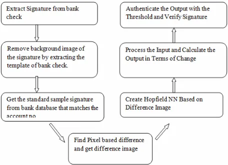
This final value will indicate unchanged (-1) or maximum change (+1); intermediate values give the strength of the change. The optimization process minimizes the energy in (2.21) starting from an initial network state. The interconnection weights in (2.25) are computed by applying data and contextual consistencies and the external inputs through the self-data information. The procedure can be depicted using following diagram in figure 2.
Training a Hopfield net involves lowering the energy of states that the net should "remember". This allows the net to serve as a content addressable memory system, that is to say, the network will converge to a "remembered" state if it is given only part of the state. The net can be used to recover from a distorted input the trained state that is most similar to that input. This is called associative memory because it recovers memories on the basis of similarity. Thus, the network is properly trained when the energy of states which the network should remember are local minima.
Figure 2: Overall processing of proposed Signature verification system based on HNN.
Each step outlined in the flow diagram (figure 2) is discussed in detail in sections 3.1 to section 3.4.
3.1 Pre-Processing and Network Initialization
The signature on the bank Cheque is always containing the back-ground, because of the reason that the Cheque leaves cannot be forged. Although this is a security feature for the bank but it leads to specific module in our system. We have to pre-process the Cheque’s image before it can be presented to the system.
The back-ground image of a signed bank Cheque’s leaf can be removed in two ways:
signature can be binarized in way that the intensity threshold removes the back-ground.
•In this method we can subtract the standard template back-ground image from the one that is signed signature, this subtraction should be done as a Homomorphic image subtraction (gray scale based using equation 2.28). For the proposed system the input image is changed based on above described method 2. The network initialization is carried out by exploiting the characteristics of the difference image. We use the initialization strategy, described in [36, 37], as follows. From the histogram of the difference image, we compute thresholds. Now, given a pixel location in the difference image, its associated node in the network is initialized based on this threshold. In the work of Wang [38], a list of major grouping principles is exhaustively studied.
In our signature verification approach, we apply the following two principles:
•Proximity
•Changed/unchanged pixels that lie close in space tend to group.
The State of each pixel is computed by HNN and its confirmation is done as based on following computations. First of all the difference image of both of the signatures (sample and test) is computed. The Difference Image is computed as:-
D(x,y) = I1(x,y) – I2(x,y) (2.28)
Here I1 and I2 are the binary Matrixes of the Learned and
test signatures. The two dimensional indices are used in terms of x and y.
Initial State of HNN is determined as = O(x,y) = 1, if D(x,y) > Threshold (changed)
= 0, Otherwise (no change) (2.29)
4.TRAINING &TEST SIGNATURE SAMPLES AND
EXPERIMENTS
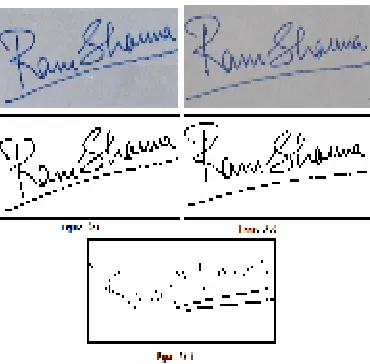
The success of any technique is closely dependent on the samples on which the experiments have been conducted. The samples of signatures were gathered from academic staff of University and Government school. The members gave signature samples on blank sheet which was cross marked but signed Cheque leaves were provided for verification purpose as well. 83 such samples were gathered and processed (see appendix 1 for samples). 40 samples were consumed during learning process of HNN where as rest of the 40 samples were used for testing of the system. Three samples were discarded because of being distorted. During the experiments one intermediate image was obtained using equation 2.28. That is a truth image; which is the simple difference image that state if the pixel is changed or not, this has been derived as a binary image. As shown in the following figures:
Figure 3(a): Sample signature of the customer stored in the Bank’s DataBase (original and binarized). Figure 3(b): Signature of the customer captured from the Cheque (original and binarized). Figure 3(c): Difference Image calculated from the difference of both binary images of the signature.
To deduce the network performance the percentage of correctly labelled pixels was computed. Correct labelling means to decide the current truth table to each of the pixel. Any pixel of the image can be labelled as one state value out of the following four:-
1. The pixel is not at all changed in both images but the HNN wrongly computes as changed.
2. The Pixel is changed and the HNN wrongly determines as unchanged.
3. The pixel is not changed in both images and HNN also states that it is not changed.
4. The pixel is changed and HNN correctly determines as changed.
So based on the knowledge of the state of each pixel we can compute the percentage of success of HNN in determination of the state, using following formula:- Perc = ((NT + PT)/(NT+PT+NF+PF))*100 (2.30) Where
NT = Negative True; i.e. number of no change pixels correctly detected by HNN
PT = Positive True; i.e. number of changed pixels correctly detected by HNN
NF = Negative False; i.e. number of no change pixels incorrectly detected by HNN
PF = Positive False; i.e. number of changed change pixels not detected by HNN
5.EXPERIMENTAL RESULTS AND DISCUSSION
The performance of the system is analysed in terms of the correct verifications, computation time and number of iteration cycles (network iterations). The table 1 shows the number of correctly verified signatures which were actually correct and incorrect and also the discarded or failed signatures which were actually correct and incorrect. This way we achieve 4 values in total. These values are presented as percentage in table 1.
Type Verified Discarded
Genuine Signatures
82% 18%
Forge Signatures 11% 89% Table 1: Signature Verification Data Result Statistics
In this table column 1 signifies the percentage of passed signatures. And Column 2 represents failed/discarded signatures. The two rows represent the type of signatures. Genuine signature means both learnt and test sample signatures are captured from the same person, so they all should be passed, but as we can see only 82 percent signatures could be verified correctly. 18 percent signatures were discarded even though they were not forged.
On the other hand we can see that in table 1 above the second row represent the signature samples which are forged at the time of testing, so the learnt signature sample and testing signature samples were gathered from different people. So ideally the system should have failed all the signatures, but only 89 percent accuracy could be obtained. The network’s learning and testing (as such recalling and threshold based verification) has been carried out in multiple sets and during each set of execution, we have taken Energy state and iterations into account. The following table (table no 2) represents the comparison between the learning and test cycle in terms of iteration cycles.
Iteration cycles
Training Data Set Energy (E x 106)
Testing Data Set Energy (E x 106)
1 -1.1167 -0.7167
2 -1.893 -1.193
3 -2.4 -1.26
4 -2.7 -2.1
5 -3.3 -2.43
6 -4.1 -2.91
7 -4.5 -3.25
8 -4.7 -3.3
9 -4.8 -3.6
10 -4.84 -3.65
Table 2: Hopfield Neural Network energy values for the training and test data sets.
The column 1 of table 2 represents the iteration number at which the energy values of both of the networks have been observed. Each of the readings mentioned in table 2 is a simple average of energy values computed for all training and test samples. Column 2 represents the energy values computed in the case of training data and column 3 represents energy values in the case of test pattern signatures.
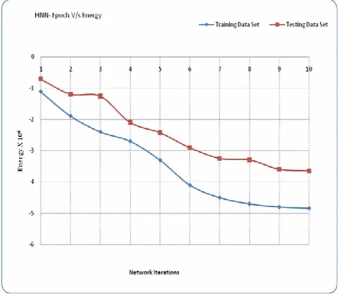
The graphical representation of data from above mentioned table 2 is shown below in Figure 4. This figure shows the average of energy values for verification of correct as well as incorrect training and testing data sets.
Figure 4: Comparison of average energy value convergence of the system with training and test samples of the signature.
Figure 4 depicts that the energy minimization in the case of training and test patterns are compared. The proposed system achieves less energy values in relatively less time and efforts in the case of training data, whereas; the test patterns consumed more time and efforts to converge. The gradual and almost constant rate of energy minimization of Hopfield neural network is observant from figure 4.
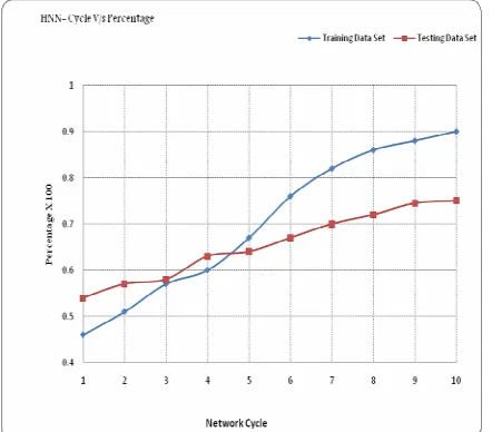
As we have discussed in section 3 that for the network’s best performance and for the judgement of test signature (in terms of forged/ passed), we compute the percentage of the correct labelling done by HNN. This percentage is also a key role player in network’s iterations. We have captured the percentage values for the network for both learning and testing samples. An average percentage is shown in table 3.
Iteration cycles
Training Data Set Percentage
Testing Data Set Percentage
1 0.46 0.54
2 0.51 0.57
3 0.57 0.58
4 0.6 0.63
5 0.67 0.64
6 0.76 0.67
7 0.82 0.7
8 0.86 0.72
9 0.88 0.745
10 0.9 0.75
Table 3: HNN correct state percentage values for the training and test data set.
test signatures. The graphical representation of data from Table 3 is shown in figure 5.
It is evident from table 3 that network takes more iterations to correctly label the test samples; one possible reason could be that we have mixed test data set with forged and genuine signatures. Due to presence of in-correct data in test data set the HNN is taking more time to correctly label all pixels / elements in test vector.
Figure 5: The Percentage values computed from equation (2.22) against the network iterations for training and test data sets.
6.CONCLUSION
In this paper, we have developed a new automatic strategy for verification of authentic signatures in bank Cheques using Hopfield Neural Networks. Some researchers have developed strategies on pattern recognition using HNN; we have extended their work for the specific area of signature verification. We have also used this kind of information for integrating the data and contextual information in form of an energy function that converges rapidly. The mapping of data information is improved in relation to classical implementations of this information. This improvement is achieved through the inter-data relations.
As it is visible from Figure 4, the convergence is fast and the results of the HNN are better in the sequence without significant illumination changes. The results in Table 2 display that the performance of network is remarkable. The best performance in terms of accuracy is obtained with iterative methods. Part of the improvement of HNN is due to the mapping of the self-information applied by HNN. This takes special relevance near the borders of changed areas. The initialization process can be important but it is not decisive. The noise removal process of the Cheque’s image is still a big challenge for this strategy.
The main drawback of Hopfield network is the high evaluation time, so for real life situations and faster responses, this strategy should be implemented on parallel architectures. As we can see from the first row of Table 1 that although, all signatures were genuine and drawn by the same person who gave learning sample; but still the system discarded 18 percent of signature samples. Similarly from the second row of table 1 we can see that the proposed
system is unable to discard 11 percent of the forged signatures. So this is the shortcoming of the proposed system and this can be further enhanced. More work needs to be carried out in this domain to get higher accuracy and great speed.
REFERENCES
[1 ].K. Franke, J.Ruiz-del-Solar, M. Koppen, " Soft- Biometics: Soft - Computing for Biometrio Applications,” ISBN - 978-3-540-43150-3, 2002. [2 ].R. Abbas, V. Ciesielski, “A Prototype System for
Off-line Signature Verification Using Multilayered Feed forward Neural Networks”, February 1995. Downloaded from:
http://citeseerx.ist.psu.edu/viewdoc/download?doi=10.1.1.47 .4751&rep=rep1&type=pdf
[3 ].R. Guest., “Age dependency in Handwritten Dynamic Signature Verification Systems”, Pattern Recognition Letters, Vol 27 , pp 1098 – 1104, 2006.
[4 ].S. Chen, Sargur Srihari, “A New Off-line Signature Verification Method based on Graph Matching”, in Proc. IEEE 18th International. Conf. on Pattern Recognition, Vol 2, pp. 869-872, 2006.
[5 ].M. Hanmandlu, M. Hafizuddin, M. Yusof, V. K. Madasu, “Off-line Signature Verification and Forgery Detection using Fuzzy Modeling”, Pattern Recognition , Vol 38, pp 341-356, 2004.
[6 ].W. Hou, X. Ye, Kejun Wang , “A Survey of Off-line Signature Verification” , in Proc. International Conference on Intelligent Mechatronics and Automation, pp 536-541, 2004.
[7 ].G. Agam, S. Suresh, “Warping-Based Offline Signature Recognition”, in Proc. IEEE Transactions on Information Forensics and Security, Vol 2, No 3, pp. 430–437 , September 2007.
[8 ].G. Agam and S. Suresh, “Particle Dynamics Warping Approach for Offline Signature Recognition”, in Proc. Conf on Computer Vision and Pattern Recognition Workshop , Vol 1, pp. 38- 45, 2006.
[9 ].A. P. Shanker, A. N. Rajagopalan, “Off-line Signature Verification using DTW”, Pattern Recognition Letters, Vol 28, pp 1407 - 1414, 2007.
[10 ]. S. Chen, S. Srihari, “A New Off-line Signature Verification Method based on Graph Matching”, in Proc. IEEE 18th International Conf on Pattern Recognition, Vol 2, pp. 869-872, 2006.
[11 ]. M. A. Ferrer , J. B. Alonso , C. M. Travieso, “Offline Geometric Parameters for Automatic Signature Verification using Fixed – point Arithmetic”, in Proc. IEEE Transaction on Pattern Analysis and Machine Intelligence, Vol 27 , No. 6, pp 993 – 997, 2005. [12 ]. E. J. R. Justino, F. Bortolozzi, R. Sabourin, “A
Comparison of SVM and HMM Classifiers in the Off-line Signature Verification” Pattern Recognition letters, Vol 26, pp. 1377-1385, 2004.
[14 ]. E. J. R. Justino, F. Bortolozzi, R. Sabourin, “Off-line Signature Verification Using HMM for Random, Simple and Skilled Forgeries”, in Proc. 6th International Conf on Document Analysis and Recognition, Vol 1, pp 1031 – 1034, Sept 2001.
[15 ]. V. Nguyen, M. Blumenstein, V. Muthukkumarasamy ,G. Leedham, “Off-line Signature Verification Using Enhanced Modified Direction Features in Conjunction with Neural Classifiers and Support Vector Machines”, in Proc. International Conf of Pattern Recognition , Vol 4 , pp. 509 – 512 , 2006.
[16 ]. H. Coetzer, R. Sabourin, “A Human – Centric Off-line Signature Verification System”, in Proc. 9th International Conference on Document Analysis and Recognition, Vol 1, pp.153 – 157, 2007.
[17 ]. C. Rabasse , R. M. Guest , M. C. Fairhurst, “A Method for the Synthesis of Dynamic Biometric Signature Data”, in Proc. 9th International Conference on Document Analysis and Recognition, Vol 1 , pp. 168-172, 2007.
[18 ]. B. Zhang, “Off-line Signature Recognition and Verification by Kernel Principal Component Self-regression “, in Proc. 5th International Conf on Machine Learning and Applications, Vol 1, pp. 28 – 33, 2006. [19 ]. J. R. Riba, A. Carnicer, S. Vallmitjana, I. Juvells,
“Methods for Invariant Signature Classification”, in Proc. 15th International Conf on Pattern Recognition , Vol 2, pp. 953-956 , 2000.
[20 ]. A. Pacut , Adam Czajka , “Recognition of Human Signatures”, in Proc. 01 International Joint Conf on Neural Networks , Vol 2 , pp. 1560-1564 , Sept 2001. [21 ]. T. Kaewkongka, K. Chamnogthai, B. Thipakorn,
“Off-Line Signature Recognition using Parameterized Hough Transform”, in Proc. 5th International Symposium on Signal Processing and its Applications”, Vol 1, pp. 451-454, 1999.
[22 ]. W. Lee, N. Mohankrishnan, M. J .Paulik , “Improved Segmentation through Dynamic Time Warping for Signature Verification using a Neural Network Classifier”, in Proc. International Conf on Image Processing , Vol 2 , pp 929-933, 1998.
[23 ]. J.-B.Fasquel, M.Bruynooghe, “A hybrid Opto-Electronic Method for Fast Off-line Handwritten Signature Verification”, IEEE Trans. International Journal on Document Analysis and Recognition, Vol 7, pp. 56-68, 2004.
[24 ]. L. Yang, “Application of HMMs for Signature Verification,” Pattern Recognition, Vol. 28, Issue 2, pp. 161-170, Feb. 1995.
[25 ]. J. J. Hopfield, “Neural network and Physical Systems with Emergent Collective Computational Abilities,” Proc. Nat. Acad. Sci. USA, Vol. 79, pp.2554–2558, 1982.
[26 ]. J. J. Hopfield and D. W. Tank, “Neural Computation of Decisions in Optimization Problems,” Biol. Cybern., Vol. 52, pp. 141–152, 1985.
[27 ]. J. J. Hopfield “Neurons with Graded Response have Collective Computational properties like those of Two-State Neurons,” Proc. Nat. Acad. Sci. USA, Vol. 81, pp. 3088–3092, 1984.
[28 ]. J. J. Hopfield and D. W. Tank, “Computing with Neural Circuits: A Model,” Science, Vol. 233, pp.625– 633, 1986.
[29 ]. D.W. Tank and J. J. Hopfield, “Simple Neural Optimization Network: An A/D Converter, Signal Decision Circuit, and Linear Programming Circuit,” IEEE Trans. Circuits Syst., Vol. CAS-33, pp. 533–541, May 1986.
[30 ]. X. C. Zeng and T. Martinez, “A New Relaxation Procedure in the Hopfield Neural Networks for Solving Optimization Problems,” Neuron Processing Letters, Vol. 10, pp. 211–222, 1999.
[31 ]. M. Ohta, A. Ogihara, and K. Fukunaga, “Binary Neural Networks with Negative Self-feedback and Its Application to N-Queens Problem,” IEICE Trans. Inform. Syst., Vol. E77-D, no. 4, pp. 459–465, 1994. [32 ]. K. Yoshino, Y. Watanabe, and T. Kakeshita,
“Hopfield Neural Network using Oscillatory units with Sigmoidal Input-Average Out Characteristics,” IEICE Trans., Vol. J77-DII, pp. 219–227, 1994.
[33 ]. Y. Watanabe, K. Yoshino, and T. Kakeshita, “Solving Combinatorial Optimization Problem using Oscillatory Neural Network,” IEICE Trans., Vol. E80-D, no. 1, pp. 72–77, 1997.
[34 ]. W. Lin, F. Liao. C. Taso, and T. Lingutle, "A Hierarchical Multiple-View Approach to Three-Dimensional Object Recognition," IEEE Tran. on Neural Net. Vol. 2 pp. 84-92, 1991
[35 ]. W. Li and M. Nasirabadi. "Object Recognition Based on Graph Matching Implemented by a Hopfield-Style Neural Network." International. J. Cor. Neural Networks 11, pp. 287-290, June 18-22, 1989.
[36 ]. L. Bruzzone and D. Fernández Prieto, “Automatic Analysis of the Difference Image for Unsupervised Change Detection,” IEEE Trans. Geosci. Remote Sens., Vol. 38, no. 3, pp. 1171–1182, Mar. 2000.
[37 ]. D.Wang, “The Time Dimension for Scene Analysis,” IEEE Trans. Neural Network., Vol. 16, no. 6, pp. 1401– 1426, Nov. 2005.
[38 ]. J. E. Slotine and W. Li, “Applied Nonlinear Control”, Prentice Hall, Upper Saddle River, NJ, 1991. [39 ]. S. R. Kosaraju, J. K. Park, C. Stein, "Long Tours and
Short Superstrings'", Proc. 35th Annual IEEE Symp. on Foundations of Computer Science, IEEE Computer Society, pp. 166-177, 1994.
[40 ]. Mérida-Casermeiro, E., Galán-Marín, G., and Muñoz-Pérez, J., “An Efficient Multivalued Hopfield Network for the Traveling Salesman Problem”, Neural Process. Letter 14, Vol. 3, pp 203-216, 2001.
[41 ]. R. D. Brandt, Y. Wang, A. J. Laub, and S. K. Mitra, “Alternative Networks for Solving the Traveling Salesman Problem and The List-Matching Problem,” in Proc. IEEE International. Conf. Neural Networks, Vol. II, San Diego, CA, 1988, pp. 333–340, 1988
Authors Biography
Gurgaon, Haryana, India as a senior software engineer. She has done her MCA from University of Rajasthan, India. She has been associated with Hughes Software Systems and Infosys. Her research areas include Handwriting recognition, Neuro-computing, Web-Acceleration and Network security.
Nipur received a PhD from Gurukul Kangri Vishwavidyalaya and an MCA from Banasthali Vidyapith. Presently she is Reader, Department of Computer Science, Kanya Gurukul Mahavidyalaya, Dehradun (second campus of Gurukul Kangri Vishwavidyalaya,Hardwar). She has 15 years PG teaching experience. Her recent research has been in the field of mobile computing & communication and interconnection networks. She handled many research projects during last ten years; Downlink Scrambling code grouping scheme for UTRA, modified generator for multiple scrambling codes, comparison of cell search methods for CDMA systems, etc She is the author of more than 35 research papers in international, national journals and conference proceedings. She is a life member of CSI & SSI and member of IEEE & IEEE Computer Society.