GSJ: VOLUME 6, ISSUE 7, JULY 2018 337
GSJ: Volume 6, Issue 7, July 2018, Online: ISSN
www.globalscientificjournal.com
On the Complete Stability Set of the First Kind for
Parametric Multi-objective Linear Programming Problems
(Parameters in the Objective Functions)
Mohamed S. A. Osman
*1, Alia Youssef Gebreel
*21 (Vice President of the Tenth of Ramadan University, Egypt), 2 (PhD in Department of Operations Research from Institute of Statistical Studies and Research (ISSR),
Cairo University, Egypt)
ABSTRACT
This paper uses parametric study for providing essential information about the problem's behavior to the decision maker. Two novel algorithms are presented in this work. The first algorithm is obtained to find the complete stability set of the first kind for parametric multi- objective linear programming problems. It is based on the weighting method for scalarizing the multi- objective linear programming problems and Kuhn- Tucker conditions for mathematical programming in general.
The second algorithm presents a technique to decompose of the parametric space in parametric linear programming problem according to the complete stability set of the first kind.
Two numerical examples are introduced to clarify the obtained results.
KeyWords
1.
INTRODUCTION
Multi-objective optimization is concerned with mathematical optimization problems involving two or more objective func-tions and constraints, which need to be optimized (minimized or maximized) simultaneously. A multi-objective problem is linear pro-gram, if all objective functions and constrains are linear *5, 9+.
These objectives are usually in incommensurate and conflicting with one another, there normally exist:
1- Infinite number of efficient (non- dominated, Pareto- optimal, or non-inferior) solutions in the MOOPs. The non-dominated set of the entire feasible decision space is called the Pareto-optimaland the boundary defined by the set of all solutions mapped from the Pareto optimal set is called the Pareto-optimal front.
2- Not all objectives can simultaneously arrive at their optimal levels. So, an assumed value function is used to choose appropriate solutions [6, 7, 8, 15].
In early work, the notions of the solvability set and the stability of the first kind are analyzed for parametric convex pro-gramming problems *12+.
The relation to the importance of the results in multi- objective convex programming problems can be seen by the funda-mental role which parametric techniques play in multi- objective programming.
In this paper, the basic concepts are defined and analyzed quantitatively for parametric multi- objective linear programming problems.
Also, the connectedness nature of the efficient extreme solutions of such problems is utilized together with the fruitful rela-tion that the Kuhn- Tucker condirela-tions play in solving such problems.
This paper is structured as follows: the parametric multi- objective linear programming problem is introduced in the second section. The third section covers the definitions with characterization of the basic notions of solvability, stability set of the first kind, and the complete stability set of the first kind for such problems. Also, an algorithm for determining the complete stability set of the first kind for a given parameter is presented. The fourth section is devoted to present an algorithm for decomposing parametric space according to the complete stability set of the first kind. Two examples are given which clarify the developed theory and algo-rithms. Finally, conclusion is reported in the fifth section.
2. Parametric multi- objective linear programming problem
Consider the following parametric multi-objective linear programming (MOLP) problem with parameters in the objective functions:
(MOLP):
Min F(λ , X) = ( ∑j=1n C1j (λ1) xj,∑j=1n C2j (λ2) xj,……,∑j=1n Ckj (λk) xj ),
Subject to
G = ,X ∈ Rn | ∑j=1n aij xj ≤ bi ,i=1, 2, …, m-
Where:
Cij (λi), i=1, 2, …,k, j=1, 2, …., n are continuous functions in λi,
,
It must be noted that the nonnegativity constraints xj ≥ 0, j=1, 2, …., n are included in the feasible region "G".
Using the weighting method to solve (MOLP) problem, we get the following single objective parametric linear programming problem "P(W)" as follows:
P(W): Min ∑i=1k ∑j=1n wi cij (λi) xj ,
Subject to
G = , X ∈ Rn | ∑j=1n aij xj ≤ bi ,xj ≥ 0, i=1, 2, …, m, j=1, 2, …., n -*13+,
∑i=1k wi = 1, wi ≥ 0, i = 1, 2, ….., k,
W= (w1, w2, ……, wk) ∈ Rk.
It is well known *4, 11+ that; if X̅ is an efficient solution of (MOLP) for λ= λ̅, then there exists W̅ ≥ 0, such that X̅ solves P(W) for λ = λ̅, and if X̅ solves P(W) uniquely for λ = λ̅, W̅ ≥ 0, or if X̅ solves P(W) for λ = λ̅, W̅ > 0 then X̅ is an efficient solution of (MOLP) for λ = λ̅. Moreover, if we take λ = λ̅, then all the efficient solutions of (MOLP) could be generated from P(W) by taking only positive values of W.
λ = (λ1, λ2, ……. ,λk) ∈ R R …, ll × l2 × × Rl.k
lk
λi ∈ R , i= 1, 2, …., k are real valued parameters,
GSJ: VOLUME 6, ISSUE 7, JULY 2018 339
3- The complete stability set of the first kind
For the parametric multi- objective linear programming problem, the following basic notions can be defined:
Definition (The solvability set)
The solvability set of problem (MOLP) which is denoted by B, is defined by:
B = , | there exists an efficient solution of problem (MOLP) for the given λ-. (2)
It is clear that if G is bounded then (3)
Definition (The stability set of the first kind)
Assume that for λ̅ ∈ B, X̅ is an efficient solution of problem (MOLP) corresponding to λ̅, then the stability set of the first kind of prob-lem (MOLP) corresponding to X̅ which is denoted by S( X̅ ) is defined by:
S(X̅) =, λ ∈ B | X̅ is an efficient solution of the problem (MOLP) corresponding to λ-. (4)
Definition (The complete stability set of the first kind)
Assume that for λ̅ ∈ B, all the corresponding efficient solutions of the problem (MOLP) are the points Xi, i ∈ L1 then the complete
sta-bility set of the first kind of problem (MOLP) denoted by SC ( λ̅ ) is defined by:
It must be noted that the efficient solutions of problem (MOLP) for any λ̅ ∈ B is connected *1, 9+, then SC ( λ̅ ) can be obtained by:
Where L is a finite set, Xi, i= 1, 2, ...., L are the efficient extreme solutions of (MOLP) corresponding to λ = λ̅.
Assume that X̅ is an efficient solution of problem (MOLP) for λ̅ ∈ B, and I = , i | ∑j=1n aij xj = bi,i=1, 2, …, m-. (7)
i.e., i denote the set of all indices corresponding to the active constraints of G at X̅ , with cardinality r. Then the corresponding Kuhn- Tucker (K.T.) conditions *3, 10+ of the P(W) for λ ϵ B takes the form:
∑i=1k wi cij (λi) + ∑ aij ui = 0, j=1, 2, ….. , n,
ui ≥ 0, i ∈ I,
where
ui , i ∈ I are the corresponding multipliers of the K.T. problem.
The equations in K.T. problemis a linear system of equations in the multipliers ui , i ∈ I which could be solved by any suitable
tech-nique from which either one of the following three cases can arise assuming the linear independence of the equations:
1) r = n
In this case ui , i ∈ I could be obtained from the equations in K.T. problem, substituting in ui ≥ 0, we get r conditions on wi , λi , i =1, 2,
…., k.
2) r < n
In this case, we use r of the n equations to get ui, i ∈ I and substituting in the rest of the equations and in the inequalities ui ≥ 0, we
get n conditions on wi , λi , i=1, 2, ….. , k.
3) r > n
In this case, n of multipliers ui, i ∈ I are obtained from the equations, and substituting in the inequalities ui ≥ 0, i ∈ I we get r
condi-tions on wi , λi , i= 1, 2, …., k.
Let A( X̅ ) = ,(W, λ) ∈ Rk× B | (W, λ) solves K.T. problem-, then the stability set of the first kind S( X̅ ) can be obtained by: S( X̅ ) = , λ ∈ B | (W, λ) ∈ A( X̅ )-. (9)
In the following, the algorithm ALg.(I) is presented to obtain the complete stability set of the first kind of problem (MOLP) for a given λ ∈ B.
ALg. (I)
1. Start with any λ̅ ∈ B.
ll × l2 × × lk
B = R R …, R.
ll × l2 × × lk
λ ∈ R R …, R
i ∈ I i ∈ L SC ( λ̅ ) = ∩ S( Xi ),
i ∈ L1 SC ( λ̅ ) = ∩ S( Xi ).
K.T. problem
(5)
(6)
2. Solve problem (MOLP) for λ = λ̅ using the multicriteria simplex method *16+ to get all the efficient extreme points of the problem "Xi", i ∈ L.
3. Put i = 1, get I1 such that
I1 = , i | ∑j=1n aij x1j = bi, i=1, 2, …., m-. (10)
4. Solve K.T. problem to get A(X1) from which we obtain S(X1).
5. Go to step (3) and put i= 2, repeat step (4) to get the set S(X2).
6. The process is repeated till all the efficient extreme points Xi, i ∈ L are exhausted.
7. The complete stability set of the first kind is obtained from the relation:
(11)
Example 1:
Let us consider the following bicriterion parametric linear programming problem with two parameters λ1, λ2 in the first objective
function f1 and one parameter λ3 in the second objective function f2. λ1, λ2, λ3 ∈ R.
MinF =( f1 = λ1 x1+ λ2 x2, f2 = - 3 x1 + λ3 x2 ),
Subject to
G = , X ∈ R2 | x1+ x2 ≤ 4,
x1+ 2 x2 ≤ 6,
x1 ≥ 0,
x2 ≥ 0-.
Since G is bounded then B = R3. If we take λ = ( λ1, λ2, λ3) = (1, 1, 1), the problem will have two efficient extreme solutions X1 = (0, 0),
X2 = (4, 0), (see Figure (1)).
(1) For X1 = (0, 0)
It is clear that I( X1) = ,3, 4-.
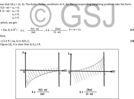
The Kuhn- Tucker conditions at X1 for the corresponding weighting problem take the form:
w λ1 – 3(1– w) – u3 = 0,
w λ2 + (1– w) λ3 – u4 = 0,
u3 ≥ 0,
u4 ≥ 0.
From which, we get:
Figure (1): G and F(G) When ( λ1, λ2, λ3) = (1, 1, 1).
GSJ: VOLUME 6, ISSUE 7, JULY 2018 341
A(X1) =,(w, λ) ∈ R4 | w(λ1 + 3) ≥ 3, w(λ3 - λ2) ≤ λ3, 0 < w < 1-. (12)
Therefore,
S( X1) =, λ ∈ R3 | (w, λ) ∈ A(X1)-. (13)
(2) For X2 = (4, 0)
It is clear that I(X2) = ,1, 4-.
The Kuhn- Tucker conditions at X2 for the corresponding weighting problem take the form:
w λ1 – 3(1– w) + u1 = 0,
w λ2 + (1– w) λ3 + u1 – u4 = 0,
u1 ≥ 0,
u4 ≥ 0.
From which, we get:
A(X2) =,(w, λ) ∈ R4 | w(λ1 + 3) ≤ 3, w(3 + λ1- λ2 + λ3 ) ≤ λ1 +3, 0 < w < 1-. (14)
Therefore,
S( X2) =, λ ∈ R3 | (w, λ) ∈ A(X2) -. (15)
The complete stability set of the first kind for the given problem for λ = (1, 1, 1) is given as
SC (1, 1, 1) = S(X1) ∩ S(X2).
4- Decomposition of the parametric space
It is clear that the parametric space is of dimension ∑i=1k λi, the solvability set B which is a subset of this space could be decomposed
according to the complete stability sets of first kind as well be clear from the following algorithm which is denoted to ALg. (II):
ALg. (II)
1. Start with any λ1 ∈ B.
2. Use ALg. (I) to get SC (λ1).
3. Choose λ2 ∈ B - SC (λ1), and use ALg. (1) to get SC (λ2).
4. The process is repeated by taking λi+1 ∈ B - SC (λi), i=1, 2, …., τ.
5. The algorithm is terminated when B - SC (λτ) = φ.
It must be noted that, the complexity of determining the complete stability set of the first kind depends mainly on the structure of Cij(λi), i=1, 2, …, k and j=1, 2, ….., n.
Remark 1:
If for any λ̅ ∈ B, X̅ is the unique efficient extreme point of problem (MOLP), then it must be noted that there is a difference between the sets S( X̅ ) and SC ( X̅ ) since S( X̅ ) gives the set of λ𝑠 that maintains X̅ as an efficient extreme point while SC ( λ̅) gives the set of
λ𝑠 that maintains X̅ as the unique efficient extreme point. In this case SC ( λ̅ ) = , λ̅ -.
Remark 2:
If at step1 of ALg. (II) for λ1 ∈ B, we get unique efficient extreme point, then choose λ2 ∈ B, λ2 ≠ λ1, and go to step1.
Example 2:
Let us consider the following bicriterion parametric linear programming problem with the same parameter λ ∈ R in the two objective functions f1, and f2.
MinF =( f1 = λ x1 + 3x2, f2 = 5 x1 - λ x2 ),
Subject to
G = , X ∈ R2 | x1+ x2 ≤ 4,
x1+ 2 x2 ≤ 6,
x1 ≥ 0,
x2 ≥ 0-.
Since G is bounded, then B ∈ R.
(1) If we take λ = 0, the problem will have one efficient extreme solution X1= (0, 0), (see Figure (2)).
It is clear that I(X1) = ,3, 4-. The Kuhn- Tucker conditions at X1 for the corresponding weighting problem take the form:
w λ + 5(1– w) – u3 = 0,
3w – λ (1– w) – u4 = 0,
u3 ≥ 0,
u4 ≥ 0.
From which, we get:
Therefore,
S( X1) =,λ ∈ R | (w, λ) ∈ A(X1) -. (18)
From Figure (3), it is clear that S( X1) ≡ R.
Then from remark 1, it follows that SC (0) = ,0-.
A(X1) = ,(w, λ) ∈ R2 | -5(1- w)
(w)
λ ≥ , ,λ (3w) (1- w) ≤ , 0 < w < 1-.
Figure (3): The Relation Between λ and W When X1= (0, 0).
-5(1- w) (w)
λ ≥ (3w)
(1- w) λ ≤
(17)
Figure (2): G and F(G) When λ = 0.
Objective space Decision space
(0, 0)
(0, 0)
(0, 20)
(0, 3)
(4, 0)
(2, 2)
GSJ: VOLUME 6, ISSUE 7, JULY 2018 343
(2) Take λ = 1, the problem will have two efficient extreme solutions X1 = (0, 0), X2 = (0, 3),
(see Figure (4)).
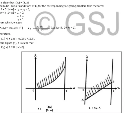
It is clear that I(X2) = ,2, 3-.
The Kuhn- Tucker conditions at X2 for the corresponding weighting problem take the form:
w λ + 5(1– w) + u2 – u3 = 0,
3w – λ (1– w) + u2 = 0,
u2 ≥ 0,
u3 ≥ 0.
From which, we get:
Therefore,
S( X2 ) =,λ ∈ R | (w, λ) ∈ A(X2) -. (20)
From Figure (5), it is clear that
S( X2 ) =,λ ∈ R | λ > 0-. (21)
(3w) (1- w) λ ≥
A(X2) = ,(w, λ) ∈ R2 | , λ ≥ 8w- 5, 0 < w < 1-.
(3w) (1- w)
Figure (4): G and F(G) When λ = 1.
λ ≥ λ ≥ 8w- 5
Figure (5): The Relation Between λ and W When X1= (0, 0), and X2 = (0, 3).
W
W
Then SC(1) = S(X1) ∩ S(X2) = ,λ ∈ R | λ > 0-. (22)
3) Take λ = - 1, the problem will have two efficient extreme points X1 = (0, 0), X3 = (4, 0), (see Figure (6)).
It is clear that I(X3) =,1, 4-. The Kuhn- Tucker conditions at X3 for the corresponding weighting problem take the form:
wλ +5(1– w) + u1 = 0,
3w – λ (1– w) + u1- u4 = 0,
u1 ≥ 0,
u4 ≥ 0.
From which, we get:
Therefore,
S( X3 ) =,λ ∈ R | (w, λ) ∈ A(X3) -. (24)
-5(1- w) (w) λ ≤
A(X3) = {(w, λ) ∈ R2 | , λ ≤ 8w- 5, 0 < w < 1}.
Figure (7): The Relation Between λ and W When X1= (0, 0), and X2 = (4, 0).
λ ≤ 8w- 5
-5(1- w) (w)
λ ≤
W
W
(23)
Figure (6): G and F(G) When λ = - 1.
Objective space Decision space
(0, 0) (0, 0)
(0, 3)
(2, 2)
(4, 0)
(- 4, 20)
(4, 12)
GSJ: VOLUME 6, ISSUE 7, JULY 2018 345
From Figure (7) , it is clear that
S( X3 ) =,λ ∈ R | λ < 0-. (25)
Then SC(-1) = S(X1) ∩ S(X3) = , λ ∈ R , λ < 0-. (26)
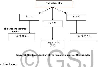
A summary of these results are shown in the following figure.
5- Conclusion
In this paper, the efficient set is studied for the parametric multi- objective linear programming problems. The aim was not only to measure and evaluate the solutions but also to determine the complete stability efficient sets of the first kind for such problems based on two new algorithms.
The problem was treated for general parameters and many special cases can be derived from this general structure. The complexity of determining the complete stability efficient set of the first kind of this problem is depended on the structure nature of the parameters.
This work could be generalized for parametric multi- objective linear programming problems with parameters in constraints, and quadratic programming problems.
Finally, this study is essentially a new trend towards a good decision for multi- objective linear programming problems.
Acknowledgment
Thanks be to ALLAH for this guidance and support in showing me the path.
References
[1] Abo-Sinna M., Amer A. H., and El Sayed H. H., "An interactive algorithm for decomposing: The parametric space in fuzzy multi-objective dynamic
programming problems", Springer Science + Business Media, LLC, 2008.
[2] Armand, P., "Finding all maximal efficient faces in multi- objective linear programming", Mathematical Programming, North- Holland, 1993, (61): 357-375.
[3] Bazzaraa, M. S., Sherali, H. D., and Shetty, C. M., "Nonlinear programming: Theory and algorithms", John Wiley & Sons, Inc., Third edition 1979, 1993, and 2006.
[4] Chankong, V. and Haimes, Y. Y., " Multiobjective Decision Making: Theory and Methodology ", Elsevier Science Publishing, 1983.
[5] De Oliveira L. Sartini, and Saramago, S. F. P.,"Multiobjective optimization techniques applied to engineering problem", J. of the Braz Soc. Of Mech.
Sci. & Eng., Vol. XXXll, No. 1/105, 2010.
The values of λ
λ = 0
λ > 0
λ < 0
,(0, 0), (0, 3)-
Unique point (0, 0) ,(0, 0), (4, 0)-
The efficient extreme points:
[6] Deb, K., Sundar J., Rao N. U. B. and Chaudhuri S., “Reference point based multi-objective optimization using evolutionary algorithms”, Intern a-tional Journal of Computaa-tional Intelligence Research, ISSN 0973-1873 Vol.2, No.3, PP. 273–286, 2006.
[7] Huang Hong Zhong, Tian Zhigang, and Zuo Ming J., “Intelligent interactive multiobjective optimization method and application to reliability
optimization”, IIE Tranction, 37, PP. 983- 993, 2005.
[8] Internet: Lecture 9: Multi-Objective Optimization (2001).
[9] Internet: McCarl Bruce A. and Spreen Thomas H., '' Chapter XI: Multi-objective programming", 1997.
[10] Mangasarian, O. L.,"Nonlinear Programming", McGraw- Hill, Inc., 1969, and the Society for Industrial and Applied Mathematices, 1994.
[11] Miettinen, K. M., "Nonlinear multiobjective optimization", Kluwer Academic Publishers, 1998, and Fourth printing 2004. [12] Osman, M. S. A., "Qualitative analysis of basic notions in parametric convex programming. II. Parameters in the objective function", Applications
of Mathematics, 1977, 5, (22): 333- 348.
[13] Osman, M. S. A., "Lecture Notes of Operations Research: Advance linear programming", Institute of Statistical Studies and Research, Cairo Univer-sity, 2013.
[14] Saad, O. M. A., "On stability of proper efficient solutions in multiobjective fractional programming problems under fuzziness", Mathematical and Computer Modelling, 2007, (45): 221– 231.
[15] Yang, Jian-Bio, and Sen P., "Preference modeling by estimating local utility functions for multiobjective optimization", European Journal of Opera-tional Research, 95 (1996) 115- 138.
[16] Yu, P. L., and ZELENY, M.," The set of all nondominated solutions in linear cases and a multicriteria simplex method", Journal of mathematical
analysis and applications, 1975, (49): 430- 468.