R E S E A R C H
Open Access
MinerLSD: efficient mining of local
patterns on attributed networks
Martin Atzmueller
1,2*, Henry Soldano
3,4, Guillaume Santini
3and Dominique Bouthinon
3*Correspondence: [email protected]
1Tilburg University, Department of Cognitive Science and Artificial Intelligence, Warandelaan 2, 5037 AB Tilburg, The Netherlands 2Université Sorbonne Paris Cité, Paris, France
Full list of author information is available at the end of the article
Abstract
Local pattern mining on attributed networks is an important and interesting research area combining ideas from network analysis and data mining. In particular, local patterns on attributed networks allow both the characterization in terms of their structural (topological) as well as compositional features. In this paper, we present MinerLSD, a method for efficient local pattern mining on attributed networks. In order to prevent the typical pattern explosion in pattern mining, we employ closed patterns for focusing pattern exploration. In addition, we exploit efficient techniques for pruning the pattern space: We adapt a local variant of the standard Modularity metric used in community detection that is extended using optimistic estimates, and furthermore include graph abstractions. Our experiments on several standard datasets demonstrate the efficacy of our proposed novel method MinerLSD as an efficient method for local pattern mining on attributed networks.
Keywords: Complex networks, Attributed networks, Closed pattern mining, Network analysis and mining, Graph mining, Community detection
Introduction
The analysis of complex networks, e.g., by investigating structural properties and iden-tifying interesting patterns, is an important task to make sense of such networks, in order to ultimately enable an understanding of their phenomena and structures, e.g., (Newman2003; Kumar et al.2006; Almendral et al.2007; Mitzlaff et al.2011; Silva et al. 2012; Mitzlaff et al.2013; Atzmueller2014; Pool et al.2014; Galbrun et al.2014; Mitzlaff et al.2014; Kibanov et al.2014; Soldano et al.2015; Atzmueller et al.2016; Bendimerad et al.2016; Kaytoue et al.2017; Atzmueller2017; 2019). In this context, data mining on such networks represented as attributed graphs has recently emerged as a prominent research topic, e.g., (Moser et al.2009; Silva et al.2012; Atzmueller2014; Galbrun et al.2014; Sol-dano et al. 2015; Atzmueller et al.2016; Bendimerad et al.2016; Kaytoue et al.2017). Methods for mining attributed graphs focus on the identification and extraction of pat-terns using topological information as well as compositional information on nodes and/or edges given by a set of attributes, e.g., (Atzmueller2018; Wasserman and Faust1994). In particular, local pattern mining focuses on the identification of dense substructures in a graph that are captured by specific patterns composed of the given attributes, e.g., for detecting communities (Moser et al.2009; Silva et al.2012; Pool et al.2014; Galbrun et al. 2014; Soldano et al.2015; Atzmueller et al.2016).
In this paper, an adapted and substantially extended revision of Atzmueller et al. (2018), we presentMinerLSDa method for the efficient mining of local patterns on attributed net-works. Compared to our work described in Atzmueller et al. (2018), we have added onto the discussion of theMinerLSDalgorithm, also considering further related approaches for putting the proposed method into context. Furthermore, we have considerably extended the evaluation and discussion of the proposed novel algorithm with new experiments, also using new (larger) datasets, and by illustrating the pattern mining approach using exemplary patterns.
MinerLSDfocuses both on local pattern mining (e.g., for local community detection) using the local modularity metric (Newman2004; Newman and Girvan2004; Atzmueller et al.2016), as well as graph abstraction that reduces graphs to k-core subgraphs (Soldano et al.2015). In order to prevent the typical pattern explosion in pattern mining, we employ closed patterns. In addition, we exploit optimistic estimates for the local modularity for focussing pattern exploration inspired by community detection methods and for pruning the pattern space. Essentially, the optimistic estimate technique provides two advantages: First, it neglects the importance of a minimal support threshold which is typically applied in pattern mining. Second, it enables a very efficient pattern exploration approach, given a suitable threshold for the local modularity, as we will show below. Then, this threshold can of course alternatively be entirely eliminated in a top-k approach. We demonstrate the efficacy of our presented novel method MinerLSD by performing experiments on several standard datasets, in relation to two baselines for local pattern mining.
Our contributions are summarized as follows:
1. For local pattern mining on attributed graphs, we analyze the impact of generating closed patterns compared to standard pattern mining in terms of the search effort. 2. Using two baseline algorithms, we further investigate the impact of pruning the
pattern exploration space using an optimistic estimate of the local modularity measure with different thresholds.
3. Finally, we propose the MinerLSD method for efficient local pattern mining on attributed graphs. MinerLSD relies on closed pattern mining, optimistic estimate pruning, and graph abstraction.
The rest of this paper is organized as follows: Section “Related Work” discusses related work, before section “Background” introduces basic notions and concepts. After that, “The MinerLSD Algorithm” section presents the novel MinerLSD method. Next, section “Datasets” introduces the applied datasets. Section “Experiments and Results” discusses our experimental results. Finally, section “Conclusions” concludes with a summary and interesting directions for future work.
Related Work
The detection of local patterns is a prominent approach in knowledge discovery and data mining, e.g., (Morik2002; Morik et al.2005; Knobbe et al.2008). Below, we discuss related work in the areas of local pattern mining, closed patterns, graph abstractions, and community detection on attributed graphs.
extends this using optimistic estimate pruning using an interestingness measure adapted from (local) community detection. In section “Experiments and Results”, we perform an extensive evaluation of the impact of closed patterns, optimistic estimates, and core structures on the pattern mining effort.
Pattern Mining
In general, local pattern mining, e.g., (Agrawal and Srikant1994; Han et al.2000; Morik 2002; Morik et al. 2005; Knobbe et al.2008; Lemmerich et al. 2012; Atzmueller2015; Lemmerich et al.2016) has many flavors, including association rule mining, subgroup discovery, and graph mining. At its core, it considers the support set of any pattern, i.e., the set of objects, often called transactions, in which the pattern occurs. The goal then is to enumerate the set of all patterns that satisfy some constraint. In the case of associa-tion rules (Agrawal and Srikant1994; Han et al.2000) typically the frequency of a pattern, or the frequency of a contained implication in the pattern, respectively, are considered. Whenever the constraint is anti-monotonic, as the frequency, a top-down search may be efficiently pruned. Still this results in investigating a lot of patterns. In the field of sub-group discovery, more complex constraints formalizx ed in quality (or interestingness) functions have been proposed; here, these do not necessarily fulfill anti-monotonicity. To handle that, optimistic estimates for those quality functions have been proposed (Wrobel 1997; Grosskreutz et al.2008; Atzmueller and Lemmerich2009; Lemmerich et al.2016) in order to efficiently prune the pattern search space. Closed pattern mining (see for instance (Pasquier et al.1999)) reduces the search by considering patterns as equivalent when hav-ing the same support set, and generathav-ing onlyclosed patterns, i.e., a most specific pattern among all equivalent patterns. Efficient enumeration algorithms have been provided, e.g., (Uno et al.2004; Boley et al.2010)). Various algorithms and methodologies using closure operators have also been proposed in the domain of formal concept analysis (Wille1982), which goes further than the enumeration alone, being interested in the lattice structure of the set of closed patterns (Ganter and Wille1999).
Local Pattern Mining on Attributed Networks
For investigating complex networks, a popular approach consists of extracting a core subgraphfrom the network, i.e., some essential part of the graph whose nodes satisfy a local property. Thek-core definition was first proposed in Seidman (1983). It requires all nodes in the core subgraph to have a degree of at least k. The idea was further extended to a wide class of so-called generalized cores (Batagelj and Zaversnik2011). The resulting subgraphs may be made of several connected components that are then considered as structural communities. However, as this may be too weak to obtain cohe-sive communities, some post-processing may then be necessary. A successful method, for example, identifies k-communities (Palla et al. 2005) that are extracted from the connected components of a graph derived from the original graph.
follows the MinerLC algorithm and adds requirements regarding the local modularity of the pattern core subgraphs. This is performed efficiently using the optimistic estimate pruning strategy of the COMODO algorithm for community detection, mentioned in section “Community Detection on Attributed Graphs”.
Community Detection on Attributed Graphs
Communities and cohesive subgroups have been extensively studied in network sci-ence, e.g., using social network analysis methods (Wasserman and Faust1994). Fortunato (2010) presents a thorough survey on the state of the art community detection algorithms in graphs, focussing on detecting disjoint communities, e.g., (Newman and Girvan2004; Fortunato and Castellano2007). In contrast to such partitioning approaches, overlapping communities allow an extended modeling of actor–actor relations in social networks: Nodes of a corresponding graph can then participate in multiple communities, e.g., (Palla et al.2007; Lancichinetti et al.2009; Xie and Szymanski2013). A comprehensive survey on algorithms for overlapping community detection is provided in Xie et al. (2013). In con-trast to the algorithms and approaches discussed above, the proposed approach utilizes further descriptive information of attributed graphs, e.g., (Bothorel et al.2015).
Attributed (or labeled) graphs as richer graph representations enable approaches that specifically exploit the descriptive information of the labels assigned to nodes and/or edges of the graph. Exemplary approaches include density-based methods, e.g., (Zhou et al.2009; Combe et al.2015), distance-based methods, e.g., (Steinhaeuser and Chawla 2008; Ge et al. 2008), entropy-based methods, e.g., (Zhu et al.2011; Smith et al.2014), model-based methods, e.g., (Balasubramanyan and Cohen2011; Xu et al. 2012), seed-centric methods, e.g., (Kanawati 2014a; Yakoubi and Kanawati 2014; Kanawati 2014b; Belfin et al.2018) and finally pattern mining approaches, which we will describe in the following in more detail.
detection and community description. A heuristic approach is applied for discovering the top-k communities, utilizing a special interestingness function which is based on count-ing outgocount-ing edges of a community similar; for that, they also demonstrate the trend of a correlation with the Modularity function.
The COMODO algorithm proposed by Atzmueller et al. (2016) applies an adapted subgroup discovery (Atzmueller and Puppe2006; Atzmueller2015) approach for commu-nity detection on attributed graphs. That is, COMODO applies subgroup discovery for detecting interesting patterns (constructed from the set of compositional attributes) for which their interestingness is evaluated on the graph topological structure. The algorithm works on an edge dataset that is attributed with common attributes of the respective nodes. Then, communities are detected in a top-k approach maximizing a given commu-nity interestingness measure. This includes, among others, the local modularity, which is derived from the (global) measure, i.e., the (Newman) Modularity (Newman 2004; Newman and Girvan2004). For an efficient community detection approach, COMODO utilizes optimistic estimate pruning.
In this paper, we adapt the COMODO approach integrating optimistic estimate pruning for the local modularity as proposed by COMODO with closed abstract pattern mining of the MinerLC algorithm. This results in the efficient and effective MinerLSD algo-rithm, making use of efficient techniques based on abstract closed pattern mining and branch-and-bound pruning according to the local modularity. At the same time, these techniques allow effective selection strategies utilizing graph abstractions together with local modularity, as we will show below.
Background
In the following, we outline the background on closed local pattern mining, introduce pruning based on optimistic estimates, and discuss pattern exploration, abstraction, and selection combining principles from pattern mining and graph mining, i.e., utilizing clo-sure on the attribute space and topological criteria based on local modularity (estimates) and k-cores.
Mining Closed Patterns to Enumerate Core Subgraphs
We consider the following general problem: LetGbe an attributed graph, i.e., a graph where each vertexvis described by an itemsetD(v)taken from a set of itemsI. We want to enumerate all (maximal) vertex subsetsW in Gsuch that there exists an itemsetq which is a subset of all itemsetsD(v),v∈ W.Wis furthermore required to satisfy some graph related constraints. In standard terminology,qis apatternthatoccursin all element ofW which is also called thesupport set or extensionext(q) of q. Efficient top-down enumeration algorithms exist as far as the constraints are anti-monotonic: whenever the constraint fails to be satisfied by some pattern, it also fails for all more specific patterns. This is obviously the case for theminimum supportconstraint that requires the size of ext(q)to be above some minimal support thresholds.
to consider graph related constraints, as for instance requiring that all vertices have a degree of at leastkin the subgroup graphGW. For that purpose, each candidate subgroup Xis reduced to its corep(X)=W using thecore operator p.
We start with the definition of closure: The operatorf that returns for any patternqthe closed patternf(q)is aclosure operator(see below) defined byf(q)=int◦p◦ext(q); the respective operators are defined as follows (note that◦denotes function composition):
• The intersection operator int(X)returns the most specific pattern occurring in the vertex subsetX.
• The core operatorp(X)returns the core, according to some core definition, of the subgraphGX ofG induced by the vertex subset X. p is an interior operator (see below).
Definition 1Let S be an ordered set and f :S→S a self map such that for any x,y∈S, f is monotone, i.e. x≤y implies f(x)≤f(y)and idempotent, i.e. f(f(x))=f(x):
- If f(x)≥x, f is called a closure operator. - If f(x)≤x, f is called an interior operator.
Essentially, core closed pattern mining relies on three main results:
1. It has been shown that wheneverp is an interior operator,f =int◦p◦ext is a closure operator (Pernelle et al.2002).
2. Furthermore, core definitions rely on a monotone property of a vertex within an induced subgraph (Batagelj and Zaversnik2002). For instance, thek -core of a subgraphGXis defined as the largest vertex subsetW⊆Xsuch that in the induced subgraphGWall verticesv have a degree of at least k. The property is monotone in the sense that when increasingGXtoGX the degree ofv cannot decrease.
3. Finally, it has been shown that the core operator which returns the core of some subgraphGX, according to a monotone property, is an interior operator (Soldano and Santini2014).
Overall, this means thatf(q)returns the largest pattern which occurs in the core of the vertex subset ext(q)in whichqoccurs. This is exploited in core closed pattern mining (Soldano et al.2017), performing a top-down search of the pattern space jumping from closed pattern to closed pattern: each closed patternqis augmented with some itemx, then the next closed patternf(q∪ {x})is computed.
Pruning Local Patterns in Graphs Using Optimistic Estimates
then pattern exploration does not need to continue for that pattern, and the search space can often be pruned significantly.
In the scope of local pattern mining on graphs, several standard community quality functions have been investigated, also specifying optimistic estimates for a number of such community evaluation functions. As shown in Atzmueller et al. (2016) these lead to a quite efficient approach for descriptive community detection using local pattern mining. In summary, using optimistic estimates we can enumerate pairs(c,W), of patterncand subgroupWinducing the subgraphGW. Then, we can select subgraphs according to an interestingness measureMof the subgraph using an anti-monotonic optimistic estimate ofMto prune the search. Additionally, a minimal support constraint can also be applied in order to improve the effectiveness of pruning.
Below, we summarize main results on using optimistic estimate pruning for community detection, specifically addressing the (local) modularity quality measure. Here, the con-cept of acommunityintuitively describes a groupW of individuals out of a population such that members ofWare strongly “connected” to each other but sparsely “connected” to those individuals that are not contained inW. This notion translates to communities as vertex setsW ⊆ Vof an undirected graphG=(V,E); in the following, we adopt the notation of Atzmueller et al. (2016) for introducing the main concepts:n:= |V|,m:= |E|, andmW := |{{u,v} ∈E:u,v∈W}|denotes the number ofintra-edgesofW.
There are different interestingness measures for estimating the quality of a commu-nity 2V →R, also according to different criteria and intuitions about what “makes up” a good community. One particular community quality function is the Modularity (Newman 2004; Newman and Girvan2004). In the context of local pattern mining, we aim to max-imizelocal quality functions for single communities. For that, we apply an adaptation of the Modularity interestingness measure, which essentially is a global measure estimating the quality of a community partitioning. Then, we focus on themodularity contribution of each individual community in order to obtain a local measure for each community, cf., (Atzmueller et al.2016), which we further calllocal modularity(MODL).
Overall, theModularityMOD (Newman2004; Newman and Girvan2004; Newman 2006) of a graph clustering withkcommunitiesC1,. . .,Ck ⊆Vfocuses on the number of edgeswithina community and compares that with theexpectedsuch number given a null-model (i.e., a corresponding random graph where the node degrees ofGare preserved). It is given by
MOD= 1 2m
u,v∈V
Au,v−
d(u)d(v) 2m
δ(C(u),C(v)), (1)
whereC(i) denotes fori ∈ V the community to which nodeibelongs.Au,vdenotes the respective entry of the adjacency matrixA.δ(C(u),C(v))is theKronecker deltasymbol that equals 1 ifC(u)=C(v), and 0 otherwise.
Themodularity contributionof a single community given by a vertex setW,W ⊆ V in alocal context(e.g., in a subgraph induced by the pattern), i.e., thelocal modularity (MODL), can then be computed (cf., (Newman2006; Nicosia et al.2009; Atzmueller et al. 2016)) as follows:
MODL(W)= mW
m −
u,v∈W
d(u)d(v)
For the above (MODL), an optimistic estimate has been introduced in Atzmueller et al. (2016). It can be derived based only on the number of edgesmWwithin the community:
oe(MODL)(W)=
0.25, ifmW ≥ m2, mW
m −
m2W
m2, otherwise.
(3)
For a detailed discussion, the derivation of the local measure, and the respective proofs, we refer to Atzmueller et al. (2016).
Local Pattern Exploration, Abstraction, and Selection
Pattern mining commonly aims at discovering a set ofnovel,potentially useful, and ulti-matelyinterestingpatterns from a given (large) data set (Fayyad et al.1996). For pattern exploration, we apply local pattern mining, in particular, (abstract) closed pattern mining (Pasquier et al.1999; Uno et al.2004; Boley et al.2010; Soldano and Santini2014; Soldano et al.2017) due to its efficient traversal of the search space for pattern enumeration and abstraction as discussed above.
Regarding pattern selection, we discuss the choices of core abstraction and modularity-based selection in the following: In contrast to many methods used in network analysis and graph mining, pattern mining on attributed graphs specifically aims at a description-oriented view, by including patterns on attributes, but also considering the topological structure. Many community mining algorithms, for example, only collect sets of nodes denoting the individual communities thus merely focusing on structural/topological aspects of the graph; typically, then there is no simple and easily interpretable description, such that a community would be represented mainly as a set of IDs, cf., (Atzmueller et al. 2016).
For local pattern mining, the goal is typically to detect a set of the most interesting pat-terns according to a given quality function, e.g., with a quality above a certain threshold, or the top-k patterns according to the ranking of the quality function denoting their inter-estingness. For subgroup discovery, as an exemplary instance, the goal is then to obtain the set of patterns covering subgroups that are “as large as possible and have the most unusual statistical characteristic with respect to the property of interest” (Wrobel1997). Thus, the interestingness of a pattern can then be flexibly defined, e.g., by a significant deviation from a model that is derived from the total population (Morik 2002; Morik et al.2005; Knobbe et al.2008). Therefore, typically the size of a pattern or the size of its extension, respectively, and the deviation compared to some null-model specifies the interestingness which is formalized in the quality function for ranking the patterns.
A thorough empirical analysis of the impact of different community mining algorithms and their corresponding objective function on the resulting community structures is pre-sented in Leskovec et al. (2010), based on the analysis of community structure in graphs (as presented in Leskovec et al. (2008)). Furthermore, Atzmueller et al. (Atzmueller and Mitzlaff2010; 2011; Atzmueller et al.2016) have empirically investigated different com-munity quality functions in the scope of local pattern mining. As shown there for the provided experiments, the local modularity quality function indicated the best results for pattern filtering and pruning in local pattern mining applications, since it provides large high quality communities, i.e., subgroups referring to the induced subgraphs, smaller patterns in terms of their description, as well as statistically significant patterns com-pared to the other mentioned quality functions which focus on smaller subgroups; those were typically also not statistically significant as specifically presented in Atzmueller et al. (2016).
Furthermore, the local modularity quality function (see Eq.2) intuitively provides the prominent property of assigning a higher ranking to larger (core) subgraphs under con-sideration, if these are considerably more densely connected than expected by chance. Therefore, these criteria conveniently capture the notion of larger subgraphs and hav-ing the most unusual statistical characteristics with respect to the null-model. In the following, we show how these criteria are directly implemented in the local modularity measure.
Consider the local modularity MODL(W) of a subgraphW:
MODL(W)= mW
m −
u,v∈W
d(u)d(v) 4m2 =
1 m
⎛
⎝mW− u,v∈W
d(u)d(v) 4m
⎞ ⎠.
Since the first factor m1 is a constant, we can consider the second factor of the former expression: It is easy to see that this factor itself is order equivalent to the local modularity function MODL, since it only depends on a fixed constant m1; by not including that it is thus not normalized relatively to the number of edges of the graph. Instead, it focuses on the number of edges of the (core) subgraph (the minuend of the term) and its deviation assessed by the null-model which is captured by the subtrahend of that term.
Thus, it is easy to see that the MODL function tends to focus on larger patterns (larger subgraphs) having the most unusual statistical characteristics with respect to the null-model. By utilizing appropriate constraints on the graph structure, e.g., using k-core abstractions we can further focus on the unusual distributional characteristics. By apply-ingk-core abstractions, for example, with increasingkwe tend to focus on increasingly denser pattern structures (subgraphs). We will also show this by our experiments in section “Experiments and Results” when we discuss our results.
which is typically applied in pattern mining, since it directly includes the size of the pat-tern as a criterion. This enables a very efficient patpat-tern mining approach, given either a suitable threshold for the local modularity, or by targeting the top-kpatterns.
The MinerLSD Algorithm
In the following, we describe our proposed novel methodMinerLSDin detail. MinerLSD integrates core subgraph closed pattern mining with pattern selection according to the local modularity MODL function, and optimistic estimate pruning according to a specific optimistic estimator, i.e., oe(MODL).
As input parameters, MinerLSD requires a graphG=(V,E), a set of itemsI, a dataset Ddescribing vertices as itemsets and a core operatorp.pdepends onGand to any image p(X) = W we associate the core subgraphC whose vertex set is vs(C) = W. In our experiments,p(X)returns the k-core ofX. As further parameters, MinerLSD considers the corresponding valuekas well as a frequency thresholds(defaulting to 0) and a local modularity thresholdlm. The algorithm outputs the frequent pairs(c,W) wherecis a core closed pattern andW = p◦ext(c)its associated k-core. For evaluation purposes, we also count the number of patterns above the local modularity threshold (#lm), and the number of patterns for which their estimate is above the local modularity threshold (#lme). It is important to note, that in the enumeration step MinerLSD ensures that each pair(c,W)is enumerated (at most) once.
MinerLSD (G, I, D, p, s, lm)
#lme←#lm←0 W ←p(V)
// also defines the associated core subgraph C=GW if|W |< soroe(MODL)(W) <lmthen exit
enum(int(W),C,∅)//int(W)is the closure of∅ _
Functionenum(c,C,EL)
ensure:outputs the frequent(c,W)pairs wherec⊇cand contains no items ofEL
Increase#lme
ifMODL(C)≥lmthen
Increase#lm andOutput(c, vs(C)) end if
for allx∈I\cdo
/* Generate all augmentations of c*/
W=p◦ext(c∪ {x})// with core subgraph Cx c←int(W)
if|W |≥sandoe(MODL)(W)≥lmandc∩EL= ∅then
enum(c,Cx,EL)
// enumerate the subtree rooted on c EL←EL∪ {x}
end if end for
_
Datasets
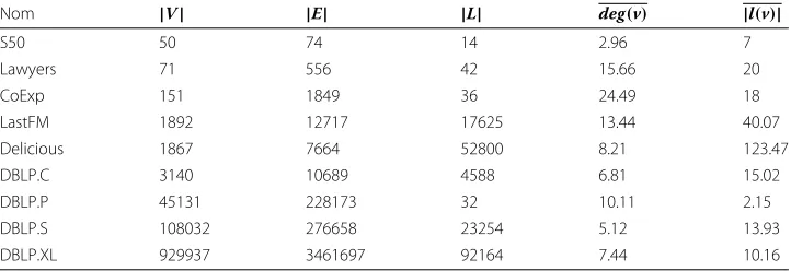
We performed our experiments utilizing a variety of attributed graph datasets ranging from small to medium graphs with small to large sets of items. Table1depicts the main characteristics of these datasets (see also (Galbrun et al.2014)), which have been previ-ously used in pattern mining tasks on attributed graphs. For each dataset, we indicate the number of edges (|E|), vertices (|V|) and labels (|L|), the average vertex degree (deg(v)) and average number of labels per vertex (|l(v)|) in the table.
• S50 is a standard attributed graph dataset used in a previous work about graph abstractions (Soldano and Santini2014).1It represents 148 friendship relations between 50 pupils of a school in the West of Scotland; the labels concern the students’ substance use (tobacco, cannabis and alcohol) and sporting activity. The values of the corresponding variables are ordered (see (Soldano and Santini2014) for details). • The Lawyers dataset concerns a network study of corporate law partnership that was
carried out in a Northeastern US corporate law firm from 1988 to 1991 in New England (Lazega2001). It concerns 71 attorneys (partners and associates) of this firm who are the vertices of four networks. In the resulting data, each attorney is described using various attributes.2We consider the advice network which is originally a directed graph in a undirected version, so that two lawyers are connected if at least one asks for advice to the other one.
• The CoExp dataset models a representative regulatory network for yeast obtained from Microarray expression data processed by the CoRegNet(Nicolle et al.2015) program. In the CoExp dataset the vertices are co-regulators and they are linked if they share a common set of target genes. The vertices are labeled with their influence profile along a metabolic transition of the organism. Each influence value represents the regulation activity of the considered co-regulator at some instant of the metabolic transition.
• LastFM, DBLP.C and DBLP.XL were used in Galbrun et al. (2014). LastFM models the social network of last.fm where individuals are described by the artists or groups they have listened to. DBLP.C contains a co-authorship graph built from a set of publication references extract from DBLP of researchers that have published in the ICDM conference. The authors are labeled by keywords extracted from the papers’ titles. DBLP.XL is the complete labeled DBLP co-authorship network used in Galbrun et al. (2014).
Table 1Datasets/Characteristics: Number of edges (|E|), vertices (|V|), labels (|L|), the average vertex degree (deg(v)), and average number of labels per vertex (|l(v)|)
Nom |V| |E| |L| deg(v) |l(v)|
S50 50 74 14 2.96 7
Lawyers 71 556 42 15.66 20
CoExp 151 1849 36 24.49 18
LastFM 1892 12717 17625 13.44 40.07
Delicious 1867 7664 52800 8.21 123.47
DBLP.C 3140 10689 4588 6.81 15.02
DBLP.P 45131 228173 32 10.11 2.15
DBLP.S 108032 276658 23254 5.12 13.93
• DBLP.P was used in Bechara-Prado et al. (Bechara Prado et al.2013). It represents a co-authorship graph built from a set of publication references extract from DBLP, published between January 1990 and February 2011 in the major conferences or journals of the Data Mining and Database communities. Three labels have been added to the original dataset based on the scope of the conferences and journals, respectively: DB (databases), DM (data mining) and AI (artificial intelligence). • Delicious consists of the social (friendship) network of the resource sharing system
delicious where individuals are described by their bookmarks’ tags. The dataset is publicly available and was obtained from the HetRec workshop (Cantador et al.2011) at Recsys 2011.3
• DBLP.S was used in Silva et al. (2012). It also represents a co-authorship network from a set of publication references extracted from DBLP.
Experiments and Results
In the following, we first summarize the applied baseline methods that were used in the comparison with the presented MinerLSD method. After that, we present our experimental results on the datasets described in “Datasets” section.
Baseline Methods
The applied set of baseline methods consists of MinerLC – an efficient algorithm for mining core closed patterns, and COMODO – an efficient algorithm for descriptive community detection using optimistic estimates.
MinerLC
MinerLC4(cf., (Soldano et al.2017)) enumerates pairs(c,W)whereGWis the core sub-graph of patternc, i.e., subgroupW = p◦ext(c)where◦is the composition operator, pis a core operatorand cis the largest pattern that occurs inW and is called a core closed pattern. A threshold on the core sizes allows to select frequent core closed pat-terns and to accordingly prune the search. The selection process relies then partly on the anti-monotonic support constraint and partly on the fact that there are less pattern core subgraphs than pattern subgraphs as various pattern subgraphsGext(q)may be reduced to the same core subgraph.
COMODO
The COMODO algorithm5presented in Atzmueller et al. (2016) performs description-oriented community detectionin order to discover the top-kcommunities. In summary, COMODO enumerates pairs(c,W)where GW is the subgraph of patternc for vertex subsetW. It selects topksubgraphs according to an interestingness measureMof the sub-graph and uses an efficient anti-monotonic optimistic estimate ofMto prune the search. Additionally, a minimal support constraint can also be applied in order to improve the effectiveness of pruning.
Similarities and Differences in Pattern Selection
Both the considered baseline methods, i.e., MinerLC and COMODO output a set of pairs (pattern, vertex subset). However, in order to compare their outputs we have to consider the following differences:
original dataset, in both connected vertices. That is, for each edge we assign the set of common items of both nodes, such that a pattern always covers two nodes connected by an edge. As a consequence,W ignores isolated nodes in which p occurs. To obtain the same vertex subset in MinerLC (and MinerLSD) it is necessary to remove isolated nodes, which is enabled by applying a 1-core graph abstraction.
• Since COMODO does not enumerate closed patterns, the same subgroup may be associated to several patterns. For that case, a post-processing is needed to eliminate the duplicates from the list of subgroups which may then be compared to the subgroups in the MinerLC pairs. This post-processing is one of the standard post-processing options of COMODO.
• MinerLC is run with a core definition while COMODO uses various parameters to limit the enumeration, as for instance thetop-k parameter.
To compare the results, MinerLC (as well as MinerLSD) should be run with the same minimum support threshold as COMODO and should only use a 1-core abstraction. The other parameters of COMODO should then have a value that does not limit the enu-meration, e.g., by providing a sufficiently large top-kparameter to enable an exhaustive enumeration.
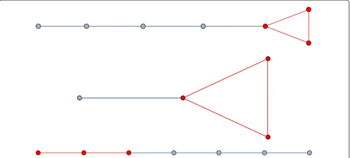
Furthermore, MinerLC and COMODO select patterns according to different criteria. This is exemplified in Fig.1, in which we have three graphs and three subgraphs induced by three vertices (in red). The subgraphG123of the top graphGis a 2-core with a local modularity of 0.178. Within the central graph, the subgraphG123is also a 2-core but with a low local modularity of -0.15. Finally, within the bottom graph,G123 is not a 2-core (since it has an empty 2-core subgraph) with a high local modularity of 0.16.
Results and Discussion
In our experiments below, we first investigate the impact of closure, before we focus on the k-core abstraction. We perform a detailed analysis of the efficiency of using the local modularity estimate for pruning the search space. Finally, we provide a structural pattern set analysis considering different metrics, and discuss exemplary patterns for illustrating the efficacy of the proposed approach.
Parameters and Datasets
For MinerLSD, it is important to note that in our experiments described below we did not have to use the minimal supports, since the local modularity threshold is efficient enough to strongly reduce the number of patterns.
Below, we consider the following pattern quantities, where the (closed pattern, support set) pairs(c,e)are output by MinerLC unless specified; also, we consider a given local modularity thresholdlm.
• #c the number of pairs(c,e).
• #lme: the number of pairs(c,e)such thatoe(MODL)(e)≥lm.
• #nec: the number of (necessary) pairs(c,e)a top-down search has to consider to ensure that no pair withoe(MODL)(e)≥lmis lost. See “Pruning: Efficiency of the
Local Modularity Estimate” section for details and results on #nec.
• #lm the number of pairs(c,e)such thatMODL(e)≥lm
• #lmeSD: the number of pairs(c,e)such thatoe(MODL)(e)≥lmas generated by COMODO.
We ran the original COMODO and MinerLC programs as available. MinerLSD is derived from the sources of MinerLC and is to be found on the MinerLC web site6. A new MinerLC version integrates the MinerLSD developments. The experimental results pre-sented here may then be obtained using appropriate parameters and options of the new software.
Impact of Closed Patterns in Reducing the Search Space
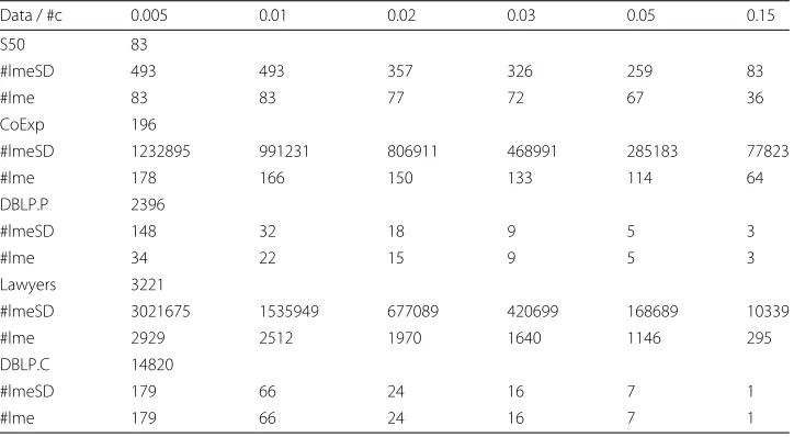
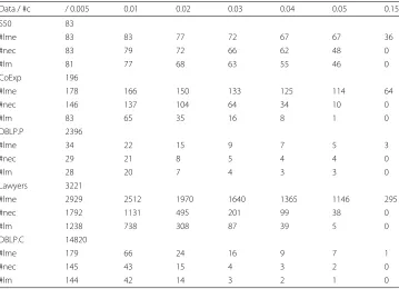
MinerLSD searches a space of closed patterns while COMODO searches the whole pattern space. Therefore, we will investigate the impact of the closure reduction, for each local modularity thresholdlm. For that, we first consider the quantity #lme of core closed patterns with a local modularity estimate above lm, as provided by MinerLSD, when using 1-cores. We consider then the quantity #lmeSD of patterns developed by COMODO using the same threshold. Table2reports #lme and #lmeSD for our datasets under investigation.
Table 2Number of patterns to develop in MinerLSD and COMODO (according to the respective local modularity threshold 0.005 ... 0.15) using a 1-core abstraction for MinerLSD
Data / #c 0.005 0.01 0.02 0.03 0.05 0.15
S50 83
#lmeSD 493 493 357 326 259 83
#lme 83 83 77 72 67 36
CoExp 196
#lmeSD 1232895 991231 806911 468991 285183 77823
#lme 178 166 150 133 114 64
DBLP.P 2396
#lmeSD 148 32 18 9 5 3
#lme 34 22 15 9 5 3
Lawyers 3221
#lmeSD 3021675 1535949 677089 420699 168689 10339
#lme 2929 2512 1970 1640 1146 295
DBLP.C 14820
#lmeSD 179 66 24 16 7 1
#lme 179 66 24 16 7 1
In the DBLP.P datasets at the contrary the items are tags, with no taxonomic order relat-ing them. Therefore, the values of #lme and #lmeSD are much closer, and even identical regarding the DBLP.C dataset.
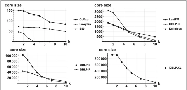
k-core sizes of the various networks
Before considering how reducing support sets to k-cores affects the number of closed pat-terns in each dataset, we consider the various networks and compute their k-core sizes for a range of values ofk. This pre-analysis aims to evaluate which level ofkwe should use in our experiments. For small datasets for which computing closed patterns does need much resources this is not that important. However, for large datasets with many attributes, i.e., potentially large numbers of closed patterns, it is much better to have a rough guideline for selecting appropriate parameters for optimizing the computational effort.
In Fig.2we display the k-core sizes for a range of values ofk, for each dataset. As we will see below, the small but densest networks for which local-modularity-based pruning has a weak efficiency, namely coExp and Lawyers, also exhibit a (relatively) slow decay with respect to increasingkvalues, whereas for the other (larger) datasets we observe a quite considerable decrease in terms of the k-core sizes.
Modularity Distributions
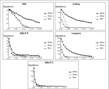
As a prerequisite for the further analysis of the local modularity optimistic estimate, we aimed to get a more detailed insight into the distribution, similar to our pre-analysis for the k-cores discussed above. Figures 3-4 show the detailed results. The plots indicate the “meaningful” values for estimating the local modularity thresholds, which support our selections of parameters in the subsequent evaluations. Furthermore, Fig. 3 also indicates the pruning potential of the local modularity threshold, even using our rather approximating sampling strategy.
Pruning: Efficiency of the Local Modularity Estimate
Fig. 2k-core sizes of the networks associated to our datasetsversus k
estimate pruning. For the other baseline, i.e., COMODO we already investigated the effi-ciency of MinerLSD which showed a considerable reduction in the number of considered patterns, cf., section “Impact of Closed Patterns in Reducing the Search Space”. Regarding the number of output patterns, both actually yield the same numbers, if a postprocessing step of COMODO is applied for keeping only the subset of closed patterns (as discussed in section “Similarities and Differences in Pattern Selection”), i.e., by considering all pairs
(c,e) with the same (vertex) subgroupeand only keeping the most specific ones. With this postprocessing COMODO returns exactly the same patterns as those output by Min-erLSD in our experiments. However, this approach is quite inefficient, cf., section “Impact of Closed Patterns in Reducing the Search Space”, since the number of considered patterns is typically considerably larger for COMODO compared to MinerLSD.
Regarding the modularity estimate, we first investigate how the local modularity con-straint affects the number of output pairs. In general, as oe(MODL) is an optimistic estimator, we may consider the best possible optimistic estimator which would only develop the #nec nodes that have at least a descendant (c,e) with local modularity MODL(e)≥lm. We have then #lm≤#nec≤#lme. Whenever #lmis far from #necthis means that there does not exist any good optimistic estimator. Whenever #lmis close to #necwhich in turn is far from #lmethis means that there could be some optimistic estima-tor that is much better than oe(MODL). By computing these numbers, we can then state separately for each dataset whether the oe(MODL)estimate is efficient in pruning the search with respect to the best possible estimatornecand whethernecwould be efficient in pruning the search, if such an estimator would be found.
Fig. 3Detailed Estimated/Observed Modularity Distributions: We consider the unlabeled graph of the dataset. We generate 100 random subgraphs of the unlabelled graph picking randomly half of the vertices. For each random graph, we compute the local modularity of the abstract 5-core subgraph and we report the survival distribution of the local modularity over the 100 experiments (in orange), i.e., for each local
modularity (lm) level, the probability of having at least that level in our sample. In blue, we report the (empirically observed) survival distribution of the local modularity, i.e., the respective MODL values of the core subgraphs of the abstract patterns discovered using the 5-core abstraction
modularity thresholdlm. In this way, we could confirm (again) that the final number of output patterns is the same for both algorithms, as discussed above.
Fig. 4Distribution of the local modularity of the 5-core abstraction in samples of 100 unlabelled random subgraphs having half of the size (number of vertices) of the original graph
develop anyway to select the 1238 patterns with local modularity MODL above 0.005. There is then a slow decrease of #lme while the decrease of #nec and #lm is much faster. Yet, pruning does still work, reducing the search effort considerably.
In contrast, for the larger datasets, e.g., for DBLP.P among the #c=2396 patterns only 34 have a local modularity estimate above 0.005, 29 of them have to be developed and 28 do have a local modularity above 0.005. Furthermore, in the DBLP.C dataset among the #c=14820 patterns only 179 have a local modularity estimate above 0.005, 145 of them
Table 3Number of patterns total, developed, necessary and with required local modularity (according to the respective threshold 0.005 ... 0.15) using a 1-core abstraction
Data / #c / 0.005 0.01 0.02 0.03 0.04 0.05 0.15
S50 83
#lme 83 83 77 72 67 67 36
#nec 83 79 72 66 62 48 0
#lm 81 77 68 63 55 46 0
CoExp 196
#lme 178 166 150 133 125 114 64
#nec 146 137 104 64 34 10 0
#lm 83 65 35 16 8 1 0
DBLP.P 2396
#lme 34 22 15 9 7 5 3
#nec 29 21 8 5 4 4 0
#lm 28 20 7 4 3 3 0
Lawyers 3221
#lme 2929 2512 1970 1640 1365 1146 295
#nec 1792 1131 495 201 99 38 0
#lm 1238 738 308 87 39 5 0
DBLP.C 14820
#lme 179 66 24 16 9 7 1
#nec 145 43 15 4 3 2 0
#lm 144 42 14 3 2 1 0
have to be developed and 144 do have a local modularity above 0.005. When the local modularity threshold increases, #lme keeps being close to #lm.
Overall, the Lawyers dataset displays moderate pruning efficiency, still allowing to avoid to develop many nodes, and this is also the case for the S50 and CoExp datasets. In con-trast, DBLP.C and DBLP.P indicate a very efficient optimistic pruning in terms of the numbers of patterns.
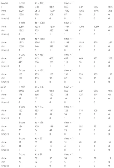
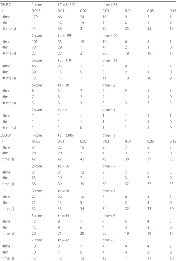
Tables4and5show the runtime results of MinerLSD for the larger of the small datasets (Lawyers, CoExp, DBLP.C, DBLP.P, runtime in seconds). Here, we observe that Min-erLSD is either in the same range or slightly faster than MinerLC for the small datasets, i.e., for Lawyers and CoExp. For DBLP.C, we observe a strongly reduced number of patterns, while the runtimes are always in the same range, especially for stronger (graph-)constraints. Here, we considered k-cores, k = 1, 2, 3, 5, 7. Therefore, while strongly reducing the number of patterns the additional computation using the estimate still keeps the runtime of the algorithm in the same range as MinerLC most of the times.
In contrast to the other smaller datasets, for the larger DBLP.P dataset we observe an increase in the runtime of MinerLSD compared to MinerLC. However, this can be explained by some special characteristic of DBLP.P. The DBLP.P dataset contains an extremely limited number of labels (32) which are used in the dataset. Here, the extra effort of the estimation does not help too much in decreasing the runtime, because the enumeration in the label space is extremely fast, and hence the check of the patterns is mainly determined by the core abstraction.
Table 4MinerLSD #lm, #lme and execution time - small datasets, compared to #c of MinerLC for same core constraints
Lawyers 1-core #c = 3221 time = 1
l 0.005 0.01 0.02 0.03 0.04 0.05 0.15
#lme 2929 2512 1970 1640 1365 1146 295
#lm 1238 738 308 87 39 5 0
time (s) 0 1 0 0 0 0 0
2-core #c = 2080 time<1
#lme 2080 1938 1670 1454 1265 1089 291
#lm 1262 775 322 104 41 7 0
time (s) 0 0 1 1 0 0 1
3-core #c = 1302 time<1
#lme 1302 1302 1215 1118 1024 920 282
#lm 1030 746 348 108 43 7 0
time (s) 0 0 1 0 0 0 0
5-core #c = 463 time<1
#lme 463 463 463 459 449 432 202
#lm 413 366 253 119 36 9 0
time (s) 0 0 1 1 0 0 0
7-core #c = 155 time<1
#lme 155 155 155 155 155 155 115
#lm 147 133 97 62 36 13 0
time (s) 1 1 0 0 0 1 0
CoExp 1-core #c = 196 time<1
l 0.005 0.01 0.02 0.03 0.04 0.05 0.15
#lme 178 166 150 133 125 114 64
#lm 83 65 35 16 8 1 0
time (s) 0 0 0 0 0 0 1
2-core #c = 172 time<1
#lme 162 153 141 125 118 108 64
#lm 89 78 51 26 12 3 0
time (s) 0 0 0 1 0 0 0
3-core #c = 138 time<1
#lme 134 129 118 109 102 95 56
#lm 75 64 42 23 12 0 0
time (s) 0 0 0 0 0 0 0
5-core #c = 62 time<1
#lme 62 60 57 51 48 47 31
#lm 31 23 12 4 2 1 0
time (s) 1 0 0 0 1 0 0
7-core #c = 37 time<1
#lme 37 37 36 34 33 32 19
#lm 27 22 17 5 3 2 0
time (s) 0 0 0 0 0 0 0
Table 5MinerLSD #lm, #lme and execution time - DBLP.C and DBLP.P, compared to #c of MinerLC for same core constraints
DBLP.C 1-core #C = 14820 time = 31
l 0.005 0.01 0.02 0.03 0.04 0.05 0.15
#lme 179 66 24 16 9 7 1
#lm 144 42 14 3 2 1 0
#time (s) 41 36 31 30 25 25 17
2-core #c = 1991 time = 20
#lme 101 35 19 10 6 5 1
#lm 78 29 11 4 2 1 0
#time (s) 23 22 21 20 18 19 15
3-core #c = 319 time = 11
#lme 46 23 11 5 4 2 1
#lm 39 15 5 3 2 1 0
#time (s) 12 11 11 11 10 10 9
5-core #c = 20 time = 2
#lme 8 3 2 2 2 1 1
#lm 7 3 2 2 1 1 0
#time (s) 3 3 3 3 3 3 3
7-core #c = 2 time = 1
#lme 1 1 1 1 1 1 1
#lm 1 1 1 1 1 1 0
#time (s) 1 1 0 1 1 1 0
DBLP.P 1-core #c = 2396 time = 9
l 0.005 0.01 0.02 0.03 0.04 0.05 0.15
#lme 34 22 15 9 7 5 3
#lm 28 20 7 4 3 3 0
time (s) 42 42 42 40 38 37 33
2-core #c = 661 time = 7
#lme 31 21 12 9 7 5 3
#lm 25 19 7 4 3 3 0
time (s) 38 39 39 38 37 37 33
3-core #c = 261 time = 7
#lme 27 20 10 7 6 5 3
#lm 21 12 5 4 3 3 0
time (s) 32 33 34 34 32 33 30
5-core #c = 84 time = 6
#lme 12 9 7 7 5 4 5
#lm 12 9 6 4 4 3 0
time (s) 20 21 20 20 19 19 17
7-core #c = 42 time = 5
#lme 10 8 7 4 4 4 2
#lm 10 7 5 4 4 3 0
time (s) 12 12 12 12 11 11 10
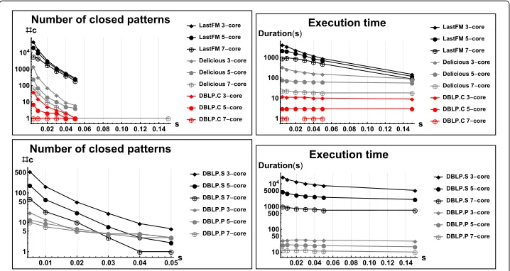
Fig. 6Number of patterns and execution time of MinerLSD on the DBLP.C, DBLP.P, Delicious and LastFM datasets with 3-cores, 5-cores and 7-cores and local modularity thresholds ranging from 0.01 to 0.15. The Y-axis of the topmost figure represents the number of closed patterns outptut by MinerLSD while the bottom figure displays the CPU time. Both Y-axis are displayed using a logarithmic scale
The benefit of applying local modularity constraints in the resulting number of closed patterns is, as expected, quite impressive. When no constraint (outside the 1-core) is applied, MinerLC in comparison finds 1,555,292 and 11,833,577 closed patterns, respec-tively. For MinerLSD, in the LastFM case there are no strong differences when using 1-cores, 2-cores and 3-cores while we know from Fig.2that using 4-cores does have an important effect. Corresponding results are also observed for larger sizes of the respec-tive k-cores. Regarding the Delicious dataset, we observe a smaller number of patterns at local modularity levels 0.04 and 0.05 with 1-cores than with 2 and 3-cores. When no local modularity constraint is applied the closed patterns with 2 and 3-cores are a subset of the closed patterns with 1-cores, therefore the results seem counterintuitive at first. However, for the same pattern the 3-core subgraph is smaller than the 1-core subgraph and may have better local modularity, which happens in the Delicious case.
runtime behavior of LastFM here is similar to DBLP.P and can also be explained by the smaller number of labels compared to Delicious. Overall, this shows that if we consider appropriate local modularity thresholds MinerLSD already allows the analysis of larger datasets, especially in terms of larger sizes of the labels, while comparable results (with respect to MinerLC) are usually obtained for weak (graph-)constraints. However, the effi-cient pruning of MinerLSD is important, e.g., for exploration, and also for the processing of larger datasets, as we will also discuss in the next section for large datasets. Detailed results are presented in Table6which also displays the #lme numbers.
Large Datasets In this section, we present experiments of MinerLSD on two large datasets, namely DBLP.S and DBLP.XL (see Table 1 for their characteristics) to fur-ther explore the scalability of MinerLSD when using bothk-core and local modularity constraints. Again we do not use any threshold on the pattern supports.
In Table7, we report the results on DBLP.S and DBLP.XL with the same local modularity thresholds as in the previous section and applyingk=1, 2, 3, 5, 7 and 7 k-core constraints, respectively. The scalability of MinerLSD depends obviously on the size and density of the network but also heavily depends on the size of the attribute set and on the average number of labels per vertex. DBLP.XL is then a real challenge as it is a large network made of 929,937 vertices related by 3,461,697 edges and described by more than 90,000 items, with an average number of 10.16 labels per vertex. The efficiency of the optimistic pruning is then of primary importance.
As can be seen in the results table, optimistic estimate pruning using local modular-ity is quite effective in achieving an efficient pattern mining approach. For both datasets, we observe large reductions in the number of patterns, while focussing on the interesting ones according to the applied local modularity interestingness measure and the utilized local modularity thresholds. In particular, the results for DBLP.S indicate the enormous pruning efficiency - here the dataset for weaker constraints cannot be handled by Min-erLC at all, where the computation did not terminate after 36 h. The DBLP.XL results indicate the same trend. Overall, this indicates the huge impact of optimistic estimate pruning using local modularity as provided by MinerLSD for handling large datasets.
Structural Pattern Set Analysis
Table 6MinerLSD #lm, #lme and execution time compared to #c of MinerLC for same core constraints
LastFM 1-core #c=1555292 time=2874
l 0.005 0.01 0.02 0.03 0.04 0.05 0.15
#lme 59528 16163 6817 3475 1920 52
#lm 17627 3633 1238 575 276 0
time (s) 5816 3400 2252 1605 1187 196
2-core #c = 471546 time = 2320
l 0.005 0.01 0.02 0.03 0.04 0.05 0.15
#lme 50507 14752 6464 3349 1856 52
#lm 16751 3646 1252 583 282 0
time (s) 4668 2915 1995 1452 1073 178
3-core #c = 161764 time = 1878
l 0.005 0.01 0.02 0.03 0.04 0.05 0.15
#lme 87211 39127 12694 5753 3039 1720 50
#lm 46400 14637 3377 1219 572 276 0
time (s) 4149 3422 2262 1596 1174 885 147
5-core #c = 26312 time = 1069
l 0.005 0.01 0.02 0.03 0.04 0.05 0.15
#lme 24807 18103 8224 4272 2352 1412 46
#lm 20562 9507 2680 1035 496 239 0
time (s) 2148 2013 1580 1206 857 706 117
7-core #c = 5859 time = 531
l 0.005 0.01 0.02 0.03 0.04 0.05 0.15
#lme 5854 5620 4031 2533 1517 994 39
#lm 5814 4482 1737 775 402 189 0
time (s) 902 953 877 738 594 486 87
Delicious 1-core #c=11833577 time=121934
l 0.005 0.01 0.02 0.03 0.04 0.05 0.15
#lme 5655 776 255 121 71 4
#lm 2214 165 31 6 1 0
time (s) 5296 2018 1173 825 643 179
2-core #c = 130458 time = 1845
l 0.005 0.01 0.02 0.03 0.04 0.05 0.15
#lme 7251 1421 288 116 65 37 3
#lm 5440 879 138 39 11 6 0
time (s) 1499 920 569 426 358 298 129
3-core #c = 11076 time = 269
l 0.005 0.01 0.02 0.03 0.04 0.05 0.15
#lme 1729 430 114 51 25 17 1
#lm 1419 311 71 25 9 6 0
time (s) 331 259 208 182 158 149 87
5-core #c = 576 time = 68
l 0.005 0.01 0.02 0.03 0.04 0.05 0.15
#lme 296 89 25 14 7 6 1
#lm 241 70 19 10 5 4 0
time (s) 77 71 66 64 62 61 55
7-core #c = 77 time = 21
l 0.005 0.01 0.02 0.03 0.04 0.05 0.15
#lme 67 41 13 7 4 1 1
#lm 66 34 10 5 2 1 1
Table 7MinerLSD #lm, #lme and execution time compared to #c of MinerLC for same core constraints
DBLP.S 1-core #c≥3457143 time = STOPPED AFTER 36h
l 0.005 0.01 0.02 0.03 0.04 0.05 0.15
#lme 1150 351 103 50 26 18 1
#lm 778 230 68 25 12 6 0
time (s) 59989 37645 24906 20634 17299 16167 8332
2-core #c≥3584834 time = STOPPED AFTER 36h
l 0.005 0.01 0.02 0.03 0.04 0.05 0.15
#lme 958 303 94 44 24 16 1
#lm 722 218 64 24 12 6 0
time (s) 36302 25949 19065 16068 13869 12907 7073
3-core #c = 1576164 time = 45720
l 0.005 0.01 0.02 0.03 0.04 0.05 0.15
#lme 621 208 72 28 17 9 1
#lm 533 165 49 20 9 6 0
time (s) 19799 15531 12329 10221 9149 8276 5143
5-core #c = 44345 time = 3791
l 0.005 0.01 0.02 0.03 0.04 0.05 0.15
#lme 200 71 26 10 6 4 1
#lm 180 59 21 7 3 2 0
time (s) 4410 3760 3173 2877 2709 2533 2044
7-core #c = 5659 time = 881
l 0.005 0.01 0.02 0.03 0.04 0.05 0.15
#lme 62 24 10 4 2 1 1
#lm 62 23 10c 3 1 1 0
time (s) 1005 908 812 784 756 687 689
DBLP.XL 7-core #c = 9206 time = 93906
l 0.005 0.01 0.02 0.03 0.04 0.05 0.15
#lme 10 5 4 3 2 1 1
#lm 9 5 3 1 1 1 0
time (s) 113790 111079 110142 107967 103363 97326 96811
Table 8Vertex Counts: Mean and standard deviation (in brackets) of the number of vertices of the pattern support, i.e., of the induced pattern subgraphs, for different values ofkand the local modularity thresholdlm
k No lm lm=0.005 lm=0.01 lm=0.02 lm=0.04
Lawyers:n=71m=556
1 12.7 (9.6) 17.2 (9.5) 20.11 (9.6) 24.4 (9.5) 29.8 (4.59) 2 15.3 (10.0) 16.8 (9.4) 19.35 (9.3) 23.4 (9.2) 27.7 (5.6) 3 18.0 (10.6) 18.0 (9.5) 19.49 (9.2) 22.9 (9.0) 26.8 (6.3) 5 23.2 (11.9) 21.7 (10.1) 21.50 (9.0) 23.7 (8.3) 27.3 (5.6)
CoExp:n=151,m=1849
1 59.5 (44.0) 51.9 (35.8) 51.5 (32.8) 54.6 (31.6) 53.9 (21.9) 2 56.9 (41.5) 49.2 (31.9) 51.9 (29.4) 57.2 (25.9) 63.0 (18.5) 3 54.7 (37.9) 47.2 (31.6) 47.4 (28.8) 52.2 (24.7) 60.2 (18.3) 5 50.0 (36.2) 48.3 (34.2) 51.6 (33.1) 54.9 (28.9) 85.5 (9.2)
DBLP.C:n=3140,m=10689
1 8.3 (30.8) 124.0 (106.1) 231.3 (144.0) 373.9 (163.6) 631.0 (63.6) 2 12.5 (68.3) 124.6 (325.9) 159.5 (103.9) 248.0 (119.0) 434.5 (64.4) 3 21.7 (126.4) 117.3 (350.3) 250.7 (549.6) 604.6 (906.4) 1256.5 (1366.8)
5 62.6 (199.6) 164.9 (327.7) 351.3 (480.6) 511.0 (555.8) 904.0 (0.0)
Pattern Selection and K-Core Abstraction
In this section, we provide examples of patterns demonstrating the benefits of pattern selection using local modularity and k-core abstraction. In particular, we discuss illus-trative examples from two different datasets – the Lawyers and the (larger) DBLP.C dataset.
Lawyers Dataset In order to demonstrate the effectiveness of the pattern exploration and selection methodology using abstract closed pattern with k-cores and local mod-ularity, we exemplify that with the two patterns shown in Fig. 7. Here, we show two similar patterns in terms of Jaccard similarity (0.52) considering the nodes of the respec-tive pattern-induced subgraphs. While the patterns are very similar regarding the overlap
Table 9Edge Counts: Mean and standard deviation (in brackets) of the number of edges of the pattern support, i.e., of the induced pattern subgraphs, for different values ofkand the local modularity thresholdlm
k No lm lm=0.005 lm=0.01 lm=0.02 lm=0.04
Lawyers:n=71m=556
1 38.2 (58.0) 61.4 (61.4) 78.4 (64.0) 103.2 (67.1) 25.6 (63.9) 2 53.8 (66.3) 62.7 (61.9) 78.3 (64.4) 104.1 (67.3) 126.1 (68.1) 3 73.2 (75.4) 72.9 (65.5) 82.2 (64.4) 104.5 (65.0) 124.8 (67.9) 5 121.7 (95.5) 109.9 (77.0) 108.2 (67.7) 123.7 (62.6) 135.7 (59.8)
CoExp:n=151,m=1849
1 365.4 (473.9) 323.1 (512.8) 327.1 (497.0) 392.0 (579.7) 448.6 (653.1) 2 404.7 (488.8) 317.2 (492.9) 325.0 (483.7) 352.2 (492.9) 377.4 (529.4) 3 445.1 (496.5) 385.1 (535.0) 375.7 (525.1) 394.6 (529.5) 481.5 (598.9) 5 525.4 (499.6) 551.8 (563.1) 625.0 (548.9) 729.3 (544.9) 1495.0 (132.9)
DBLP.C:n=3140,m=10689
1 7.4 (91.4) 164.9 (192.5) 347.3 (282.5) 627.8 (340.3) 1278.0 (356.4) 2 22.8 (240.5) 316.81 (1183.3) 349.2 (271.3) 577.7 (328.6) 1126.0 (357.8) 3 66.7 (531.01) 419.7 (1487.5) 945.3 (2350.3) 2393.0 (3924.2) 5229.0 (5897.3)
Table 10Scaled Graph Densities: Mean and standard deviation (in brackets) of the scaled densities of the pattern support, i.e., of the induced pattern subgraphs, for different values ofkand the local modularity thresholdlm
k No lm lm=0.005 lm=0.01 lm=0.02 lm=0.04
Lawyers:n=71m=556
1 4.59 (2.63) 6.34 (2.51) 7.26 (2.46) 8.13 (2.61) 8.98 (3.27) 2 5.92 (2.56) 6.63 (2.47) 7.50 (2.38) 8.50 (2.42) 9.43 (2.82) 3 7.23 (2.47) 7.42 (2.32) 7.92 (2.27) 8.80 (2.27) 9.45 (2.67) 5 9.89 (2.28) 9.74 (2.10) 9.82 (1.96) 10.38 (1.80) 11.38 (1.95)
7 12.23 (2.08) 12.15 (2.05) 11.99 (1.86) 12.20 (1.40) 13.14 (1.20) CoExp:n=151,m=1849
1 9.58 (8.34) 9.38 (9.54) 10.14 (9.83) 11.17 (11.12) 12.19 (13.90) 2 11.15 (8.37) 9.78 (9.09) 10.14 (9.18) 10.41 (9.85) 10.19 (11.46) 3 13.07 (8.60) 12.02 (9.66) 12.15 (9.83) 12.22 (10.44) 13.22 (13.20)
5 17.92 (8.25) 18.40 (9.00) 20.68 (8.50) 25.22 (5.72) 35.42 (0.71) DBLP.C:n=3140,m=10689
1 1.73 (0.57) 2.60 (0.82) 2.93 (0.75) 3.38 (0.65) 4.02 (0.73) 2 3.15 (0.68) 4.15 (0.98) 4.33 (0.72) 4.66 (0.68) 5.13 (0.89)
3 4.73 (0.87) 5.90 (0.78) 6.35 (0.79) 6.74 (1.14) 7.89 (0.80) 5 7.30 (1.57) 8.55 (1.94) 10.16 (2.02) 10.92 (2.17) 12.45 (0)
and their size, they have quite different local modularity values referring to their connec-tivity structure. The left pattern described by 35 < Age≤ 65 ANDSeniority < 5 AND Status = Partner, with asize = 24 of the set of nodes in its subgraph, is considerably denser with a local modularity of MODL=0.058, compared to the pattern on the right; the latter is described byAge< 40 ANDSeniority≤30, with asize =23 of the pattern support and a local modularity of only MODL=0.013. Therefore, while both patterns are abstract closed patterns according to similar support criteria and the 5-core abstraction, a higher modularity threshold, e.g., MODL≥0.05 would only select the first (left pattern in Fig.7) instead of the right pattern. From the description, we can also observe that the
Table 11Ratio of outgoing edges to edges in the pattern subgraph (in-edges): Mean and standard deviation (in brackets) of that ratio of the pattern support, i.e., of the induced pattern subgraphs, for different values ofkand the local modularity thresholdlm
k No lm lm=0.005 lm=0.01 lm=0.02 lm=0.04
Lawyers:n=71m=556
1 10.99 ( 9.07) 4.90 (2.55) 3.68 (1.72) 2.68 (1.19) 1.80 (0.65) 2 6.58 (4.40) 4.81 (2.53) 3.67 (1.72) 2.64 (1.16) 1.81 (0.65) 3 4.62 (2.81) 4.14 (2.18) 3.46 (1.58) 2.58 (1.10) 1.84 (0.66) 5 2.74 (1.62) 2.82 (1.53) 2.69 (1.32) 2.19 (0.89) 1.56 (0.52)
CoExp:n=151,m=1849
1 4.95 (8.72) 2.46 (1.59) 2.13 (1.36) 1.62 (1.11) 0.69 (0.34) 2 3.88 (4.76) 2.69 (1.79) 2.48 (1.52) 2.24 (1.35) 1.69 (1.10) 3 3.58 (4.48) 2.83 (2.33) 2.58 (1.77) 2.41 (1.49) 1.82 (1.14) 5 3.75 (4.12) 2.89 (2.75) 2.24 (2.04) 1.57 (1.07) 0.16 (0.10)
DBLP.C:n=3140,m=10689
1 14.23 (13.72) 6.85 (1.94) 5.28 (1.19) 3.94 (0.80) 2.39( 0.41) 2 11.29 (10.37) 5.99 (2.09) 4.88 (1.17) 3.78 (0.77) 2.44 (0.50) 3 11.44 (8.04) 5.96 (1.90) 4.57 (1.64) 2.96 (1.82) 1.27 (1.68)
Fig. 7Example patterns from the Lawyers dataset: Both patterns are similar 5-cores, with a Jaccard similarity considering the nodes of the respective pattern-induced subgraphs of 0.52. The pattern on the left (described by 35<Age≤65 ANDSeniority<5 ANDStatus=Partner, withsize=24) is considerably denser with a local modularity of MODL=0.058, compared to the pattern on the right (described byAge<40 AND
Seniority≤30, withsize=23) which only has a local modularity of MODL=0.013. In the figures, we depict in red the edges and the vertices in the pattern extension, in gray the out-edges of the pattern (i.e., one vertex of a gray edge is contained in the pattern subgraph and the other vertex is not) and in light gray the rest of the graph
selected (left) pattern is more interesting, since it provides a more precise description. In the figures, we depict in red the edges and the vertices in the pattern subgraph; in gray, we show the out-edges of the pattern (i.e., one vertex of a gray edge is contained in the pattern extension and the other vertex is not); in light gray we depict the rest of the graph.
DBLP.C Dataset In order to show the impact of pattern selection and k-core abstrac-tion, we first consider the local Modularities onk-cores with increasingk. For analyzing the impact of thek-cores we firstly consider the empty pattern, thus only focussing on the abstraction by the appliedk-core. For the local modularity values of the empty pat-tern, fork = 2, 3, 4, 5 we observe MODL = 0.0075, 0.0430, 0.0915, 0.1223, respectively. Thus, we observe the clear trend that increasingk yields patterns with higher connec-tivity structures as shown by the increasing local modularity values; similar trends are obtained for the other datasets. This complements our results in the last section, where we discussed, how increasingkfor the k-core abstraction together with increasing local modularity thresholds focuses on larger and more “interesting” patterns as measured by the local modularity quality function.
Fig. 8Illustrative patterns (DBLP.C). Left: 5-core empty pattern with a local modularity of MODL=0.1223; middle: 3-core empty pattern with a local modularity of MODL=0.0430; right: 3-core “mine” pattern with a local modularity MODL=0.0503. In the plots, red color indicates the core graph (i.e., the in-edges of the pattern), blue color shows the edges incident to the nodes of the core graph, gray depicts the edges of the rest of the graph
left plot in Fig.9shows the “mine” pattern in detail, as a “zoom-in” focussing on all edges incident to nodes contained in the pattern subgraph.
Figure9illustrates the selection process for different 3-core patterns in detail, provid-ing the “mine” pattern (coverprovid-ing 290 vertices and 1059 edges, MODL = 0.0503) that is selected according to a local modularity thresholdlm=0.04 and the “algorithm” pattern (covering 45 vertices and 93 edges, MODL = 0.0072) which is a further specialization of the 3-core empty pattern. As we can clearly observe for the “mine” pattern, its struc-ture is more interesting concerning its connectivity – i.e., its distributional unusualness compared to the expectation modeled by the null-model. This is a representative illustra-tion, how the proposed approach using local modularity pruning achieves a better pattern selection method for the same core constraint(s).
Conclusions
In this paper, we have proposed the novel MinerLSD method for efficient local pattern mining on attributed networks. It enumerates local patterns and associated subgroups in
attributed networks, utilizing different pattern and graph mining techniques. In particu-lar, MinerLSD is based on three main basic ideas: First, enumerating only closed patterns, which is particularly beneficial whenever items have dependencies. This occurs as soon as some attributes, either numeric or hierarchical, have to be translated into various items to express interesting patterns, e.g., interrelated intervals and hierarchical dependencies. Second, we focus on reducing pattern subgraphs to core subgraphs which allows both to strongly reduce the number of patterns and to focus on essential parts of graphs. Third, we select cohesive subgraphs during the search according to topological quantities as local modularity and, above all, to allow pruning by using optimistic estimates of the local modularity measure.
We performed a set of experiments in order to estimate the impact of the investigated approaches, for which we included two baseline methods, i.e., MinerLC and COMODO for comparison. The purpose was then to investigate i) the pruning efficiency of Min-erLSD using the local modularity estimate as implemented in COMODO, ii) the impact of searching for closed patterns (as implemented in MinerLC) and therefore enumerat-ing only the cohesive subgraph associated to the patterns, and iii) the added potential for pattern selection based on the combination of both k-core abstraction and local modular-ity selection. The latter allows to strongly reduce the number of patterns while focussing on essential parts of the graph which leads to more interesting high quality patterns. For our experiments we used a number of datasets with different characteristics, also ranging from small to large datasets in order to estimate the scalability of MinerLSD. Overall the result indicated effects that were always positive, and sometimes even crucial, for allow-ing to handle even rather complex and large datasets with reasonable pattern set sizes and computational effort – without using any minimum support threshold. Specifically, the results of our experiments show the efficiency of the presented method. Further-more, we have presented exemplary results showing the benefit of pattern selection and abstraction which demonstrate the efficacy of the proposedMinerLSDapproach. Over-all, by implementing the different ideas. and techniques summarized above in the novel MinerLSDmethod, i.e., utilizing closed patterns, graph abstractions, optimistic estimate pruning using local modularity), we obtain a very flexible tool that allows to handle large graphs with adequate constraints on the subgroups and patterns to discover.
For future work, we intend to characterize the attributed graphs in terms of which prun-ing method is especially efficient, and to investigate other measures than local modularity in order to estimate their pruning efficiency. Furthermore, we aim to investigate other core definitions than k-cores as well. Also, focussing on sets of (local) patterns, and their relations, in order to obtain, e.g., the most diverse, representative, interesting, and rele-vant results, cf., (Knobbe and Ho2006; Lemmerich et al.2010; Van Leeuwen and Knobbe 2012; Atzmueller et al.2015) is a further interesting research direction to consider.
Endnotes 1Available at:
http://www.stats.ox.ac.uk/~snijders/siena/s50_data.htm 2Available at:
https://www.stats.ox.ac.uk/~snijders/siena/Lazega_lawyers_data.htm 3https://grouplens.org/datasets/hetrec-2011/