Improved feature extraction and matching in urban environments based
on 3D viewpoint normalization
Yanpeng Cao
⇑, John McDonald
Department of Computer Science, National University of Ireland Maynooth, Co. Kildare, Ireland
a r t i c l e
i n f o
Article history: Received 29 March 2010 Accepted 12 September 2011 Available online 1 October 2011 Keywords:
Feature extraction Wide baseline matching 3D viewpoint normalization Monocular 3D reconstruction Urban navigation
a b s t r a c t
In this paper we present a novel approach for generating viewpoint invariant features from single images and demonstrate its application to robust matching over widely separated views in urban environments. Our approach exploits the fact that many man-made environments contain a large number of parallel lin-ear features along several principal directions. We identify the projections of these parallel lines to recover a number of dominant scene planes and subsequently compute viewpoint invariant features within the rectified views of these planes. We present a set of comprehensive experiments to evaluate the performance of the proposed viewpoint invariant features. It is demonstrated that: (1) the resulting feature descriptors become more distinctive and more robust to camera viewpoint changes after the pro-cedure of 3D viewpoint normalization; and (2) the features provide robust local feature information including patch scale and dominant orientation which can be effectively used to provide geometric con-straints between views. Targeted at applications in urban environments, where many repetitive struc-tures exist, we further propose an effective framework to use this novel feature for the challenging wide baseline matching tasks.
Ó2011 Elsevier Inc. All rights reserved.
1. Introduction
The motivation of our works is to develop a vision-based system to facilitate intelligent navigation applications within cities. The idea is that the user could arbitrarily capture an image in urban environment and compare it against a database of stored landmark images in order to determine the camera pose within the world coordinate frame. Navigation information could be projected into the image (e.g. augmented reality) and then transmitted back to the user. In such system robust image matching is a crucial func-tionality. Previously a number of successful image matching tech-niques[1–6]have been proposed – a comprehensive review was given in[7]. These methods usually consist of finding stable and repeatable regions of interest, followed by computing feature descriptors that characterize the local appearances in some invari-ant manners. The underlying principle for achieving invariance is to normalize the extracted regions of interest so that the appear-ance of a region will always produce the same descriptor (in an ideal situation) under the changes of illumination, scale, rotation, and viewpoint. However, the performances of the existing 2D fea-tures drop significantly under substantial camera viewpoint changes[8]. The same object will appear very different when cam-era viewpoint is significantly changed. Using descriptors directly
computed on such wide baseline images, it is difficult to establish correct matches. In this paper we combine recent advances in 2D feature extraction with the concept of 3D viewpoint normalization to improve descriptive ability of local features for robust matching over largely separated views.
General 3D reconstruction based on single monocular images is a difficult task since the depth information remains ambiguous without the provision of further image cues. In this paper, we in-clude following prior knowledge and assumptions to enable the task in man-made environments. First, we assume that the build-ing facades are piecewise planar, and a number of dominant 3D planes can be used to approximate the spatial layout of buildings. In man-made environments, this approximation yields good per-formances. Second, the building facades usually contain a large number of parallel lines along several principal directions. The images of these 3D parallel lines and their corresponding vanishing points provide valuable cues for 3D recovery. Third, we assume that the buildings have vivid enough vertical boundaries and their images are captured using a nearly upright camera thus the verti-cal direction can be robustly detected.
In this paper we propose an effective method to recover a num-ber of 3D planes from single 2D images of urban environments and then use them to describe the spatial layout of the imaged scenes. The extracted regions of interest can be normalized with respect to these recovered 3D planes to achieve viewpoints invariance. Spe-cifically, line segments are extracted in an image and subsequently 1077-3142/$ - see front matterÓ2011 Elsevier Inc. All rights reserved.
doi:10.1016/j.cviu.2011.09.002
⇑Corresponding author.
E-mail addresses:[email protected](Y. Cao),[email protected](J. McDonald).
Contents lists available atSciVerse ScienceDirect
Computer Vision and Image Understanding
j o u r n a l h o m e p a g e : w w w . e l s e v i e r . c o m / l o c a t e / c v i ugrouped into several principal directions by identifying common vanishing points. In this step we include an effective tilt rectifica-tion procedure to improve results. Then we take into account both the distribution of line segments and the possible shape of building structure to obtain a reasonable 3D understanding of the imaged scene. As the last step, the individual patches on the original image, each corresponding to an identified 3D planar region, are rectified to form the front-parallel views of building facades. Viewpoint invariant features are then extracted on these rectified views to provide a basis for further matching. The key idea of the proposed method is schematically illustrated in Fig. 1. This novel feature scheme has many advantages over other conventional 2D features (e.g. SIFT[3]). First of all, the resulting features are very robust to large viewpoint changes after viewpoint normalization. Also, the features contain robust local patch information for generating geo-metric constraints between views. This makes viewpoint invariant features particularly suitable for image matching in urban environ-ments where substantial repetitive structures exist.
The main contribution of this paper is threefold. First, we pres-ent a novel approach for generating viewpoint invariant features from single images taken in urban environments. Compared with some previous works on combining 2D features with 3D geometry [9,10], our method only requires a single image, does not need information from additional devices, and thus it offers wider appli-cability. Second, we make systematical performance evaluations of the proposed viewpoint invariant features. To the best of our knowledge, this paper is the first to provide a quantitative analysis of the performance gain of combining 2D features and 3D geome-try. It is demonstrated that (1) after viewpoint normalization the resulting descriptors remain more invariant to viewpoint changes; (2) for all ground truth correspondences the scale ratios and dom-inant gradient orientations are equal up to a small tolerance. These improvements intuitively prove the feasibility of the one-point RANSAC algorithm explained in [10]. Third, we further propose an effective framework to use this novel feature for challenging wide baseline matching tasks in urban environments where many repetitive structures exist.
The remainder of the paper is organized as follows. Section2 re-views some existing approaches for feature extraction and 3D reconstruction. The procedures of generating viewpoint invariant features, which include line segments grouping, 3D reconstruction and viewpoint normalization, are explained in Sections 3–5, respectively. In Section6, the performance of viewpoint invariant features is comprehensively evaluated. We further propose an effective framework to use this novel feature for matching repeti-tive structures in urban environments in Section 7. Finally, con-cluding remarks and future works are provided in Section8.
2. Related works
A large number of papers have been reported on robust 2D im-age feature extraction. For a detailed review see[7]. Among them the SIFT (scale-invariant feature transform) feature [3]is widely used due to its superior performance under changes of illumina-tion, viewpoint, scale and rotation. The potential keypoints are firstly identified by searching for local extreme in a series of Differ-ence-of-Gaussian (DOG) images. Next, local image patches at these locations are normalized to achieve invariance up to a 2D similar-ity. Finally, a 128-element SIFT descriptor is computed to charac-terize the local patch appearance which can be subsequently used for feature matching. In[11]the authors conducted a compre-hensive evaluation of various feature descriptors and concluded that the 128-element SIFT descriptor outperforms other schemes. SIFT feature has been successfully applied to various computer vi-sion tasks such as object recognition, 3D modeling, and pose esti-mation. However, the performance of SIFT drops quickly under substantial viewpoint changes, since the change of camera position induces apparent projective distortion into the image.
Recently, many researchers have proposed to use the 3D object geometry as an additional cue to improve 2D feature matching. A novel feature scheme, Viewpoint Invariant Patches (VIP), based on 3D normalized patches was proposed for 3D urban model matching and querying[10]. In[9], both texture and depth infor-mation were exploited to compute a normal view onto the surface. In this way they kept the descriptiveness of similarity invariant features (e.g. SIFT) while achieving extra invariance against per-spective distortions. In [12], 3D gradients and histograms were considered to generate 3D features which are invariant to changes in rotation, translation, and scale. However, in these methods 3D geometry information needs to be acquired in advance using either multiple views (SfM or stereo vision) or additional active sensors (Lidar or Radar). The idea of singe-image based 3D viewpoint nor-malization was previously proposed in [13]. However, they only make use of the improved feature descriptors to enable wide base-line image matching. As pointed out in [10,14], both patch scale and feature orientation provide valuable information for geometric verification which should be made good use of.
Previously a number of techniques have been developed for 3D reconstruction using monocular cues. Hoiem and his research group estimated the coarse 3D properties of a scene by learning appearance-based models of geometric classes, and then used the recovered 3D geometry to improve the performance of computer vision applications such as object detection and single view recon-struction[15–18]. In[19], a supervised learning approach was pro-posed for 3D depth estimation via the use of Markov Random Fields. Usually architectural scenes are highly constrained, thus their images contain many regular structures including parallel lin-ear edges, sharp corners, and rectangular planes. The presence of such structures suggests opportunities for constraining and there-fore simplifying the reconstruction task. A number of techniques [20,21,6] were proposed for detecting rectangles aligned with principal directions using the recovered vanishing points. Such Fig. 1.The major steps involved viewpoint invariant feature extraction and
structures provide strong indications of the existence of co-planar 3D points. In[22–24], rigidity constraints on parallelepipeds were exploited to infer adequate information for camera calibration and 3D reconstructions using single images. In[25], the authors used the normals of building facades to represent their 3D layouts. The linear constraints such as connectivity, parallelism, orthogo-nality, and perspective symmetry, were imposed on the object shape formulation and the optimal solution was obtained for 3D reconstruction. In [26], visually pleasing urban 3D models were generated from single images by solving the problem of model fit-ting. Assuming the environment is composed of a flat ground plane and vertical walls, they used a continuous polyline to parameterize the ground-vertical boundary. The success of the above approaches inspired us to extend the conventional 2D image features to the third dimension using the obtained 3D geometry from single images.
This paper is built upon our previously proposed method[27]and is further extended in twofold. First, we perform a systematic eval-uation of the proposed viewpoint invariant features. To the best of our knowledge, this paper is the first comprehensive quantitative evaluation of using 2D image texture together with 3D object geom-etry. We demonstrate the resulting descriptors after viewpoint nor-malization remain more invariant when viewpoint changes. Also, it is shown that for all ground truth correspondences their scale ratios and dominant orientations are equal up to a small tolerance. These results experimentally verify the feasibility of the one-point RAN-SAC algorithm[10]. Second, targeted at applications in urban envi-ronments where many repetitive structures exist, we propose an effective framework to use this novel feature for wide baseline matching. We accept multiple matches to cope with repetitive urban structures and then make use of the information (patch scale, dom-inant orientation, feature coordinates) associated with the extracted viewpoint invariant features to identify correct ones.
3. Line segments grouping
Given images taken in urban environments, we apply the ap-proach described in [20] for line extraction. Strong edge pixels are detected using the Canny edge detector and those with similar gradient directions are merged together to generate a number of straight lines. For better efficiency, only the line segments of length greater than 30 pixels are kept for further analysis. In our experi-ments this typically results in 200–400 line segexperi-ments extracted per image (640480 pixels).
Next the line segments corresponding to building parallel edges are identified and further grouped into principal directions. An effective approach is proposed to this problem by adapting the ap-proaches described in[28,26,20]. The method contains two major steps: (1) select the images of vertical line segments and use them to rectify camera tilt; (2) identify the horizontal parallel lines and group them into principal directions. The details of each step are presented in the following subsections.
3.1. Tilt rectification
We rectify camera tilts to make 3D vertical boundaries of build-ings also appear vertical in 2D images. To do this, we start by con-sidering a general 34 matrixPthat projects a homogeneous 3D world pointX= [X,Y,Z,1]Tinto the 2D image plane. Without loss of generality, we coincide the camera center with the world origin as:
x y 1 2 6 4 3 7 5’P X Y Z 1 2 6 6 6 4 3 7 7 7 5¼K ½Rj0 X Y Z 1 2 6 6 6 4 3 7 7 7 5¼KR X Y Z 2 6 4 3 7 5 ð1Þ
where’denotes equality up to scale,Kis the camera intrinsic cal-ibration matrix andRis the 33 camera rotation matrix. We can decomposeRinto three rotation matrices corresponding to the roll (/), pitch (h), and yaw (
w
) angles as:x y 1 2 6 4 3 7 5’KR/RhRw X Y Z 2 6 4 3 7 5 ð2Þ
We seek a 33 homographyHtiltto compensate the non-zero pitch
and roll angles as:
Htilt¼KRh1R 1
/ K 1
ð3Þ
After applyingHtiltto the original image, as shown in Eq.(4), a 3D
vertical line (with constantXandZcoordinates) will appear vertical in the wrapped 2D image (having the samex0 coordinate in the wrapped image). Htilt x y 1 2 6 4 3 7 5’KRw X Y Z 2 6 4 3 7 5¼K coswXsinwZ Y sinwXþcoswZ 2 6 4 3 7 5’ x0 y0 1 2 6 4 3 7 5 ð4Þ
The algorithm for tilt rectification is given as follows:
1. Select approximately vertical lines in the image (lines within ±
p
/6 radians of the vertical image direction) and apply the RAN-SAC technique[29]to find the vertical vanishing point and its corresponding line segments (the images of building vertical edges). Record the endpoint coordinates of these line segments. 2. Normalize all endpoint measurements by pre-multiplying thembyK1. A simplified camera model is used as:
K¼ f 0 0 0 f 0 0 0 1 2 6 4 3 7 5 ð5Þ
where we assume the image skew is zero, the aspect ratio is one, and the camera principal point coincides with the image center [30]. The unknown camera focal length can either be retrieved from the provided EXIF file (available for most modern digital cameras) or be estimated using the existing camera self-calibra-tion techniques[31,28,20,32].
3. Find the optimal estimates of pitch and roll angles so that the resulting rotation matrix will transform the images of 3D verti-cal lines to appear vertiverti-cal in the rectified view. Specifiverti-cally, we apply nonlinear least-squares optimization to estimate the rota-tion matrix which minimizes the column coordinate differences between two endpoints of all selected line segments.
4. Compute the homographyHtiltfor tilt rectification as shown in
Eq.(3)and apply the transformation to the original image to create a tilt rectified view where keystone effect is removed. 3.1.1. Performance evaluation
We tested the proposed tilt rectification method on building images from the ZuBud dataset[33]. Since the camera focal lengths are not provided in the dataset, we apply a simple technique de-scribed in[31]to compute them independent of the method. Given vanishing pointsV1¼ ½xv1;yv1;1
T
andV2¼ ½xv2;yv2;1
T
from two orthogonal directions, focal length fcamera can be estimated as
follows:
xv1xv2þyv1yv2þf
2
camera¼0)fcamera¼ ffiffiffiffiffiffiffiffiffiffiffiffiffiffiffiffiffiffiffiffiffiffiffiffiffiffiffiffiffiffiffiffiffiffiffiffixv1xv2yv1yv2
p ð6Þ
In our implementation fcamera typically ranges between 600 and
1200 pixels. For 1005 urban building images in the ZuBuD dataset, the distribution of the calculated focal lengths is shown inFig. 2.
Next we calculated the average column coordinate differences between two endpoints of the vertical line segments before and after tilt rectification. The quantitative results are given inFig. 3. Fig. 4shows some example results of tilt rectification. The keystone effects are very obvious in the original images (a rectangle struc-ture will appear trapezoidal which is wider at the bottom in case of camera pitching up). After rectification, the images of vertical world lines become much more parallel to the image columns. The building boundaries will appear vertical in the rectified image, making the building structure more evident. We can divide an im-age into several vertical strips where each strip represents a single 3D plane of the building surfaces.
3.2. Line grouping
Urban environments usually contain a good number of parallel building edges. The images of a group of 3D parallel lines will inter-sect into a common vanishing point. We propose to group the hor-izontal parallel lines into several principal directions by identifying such common vanishing points. In practice, this is a challenging task for two major reasons: (1) a large number of outliers occur in natural scenes (e.g. due to foliage, people, other facades, etc.); (2) any two non-collinear lines will generate a possible vanishing point at their intersection which will produce too many candidates to verify.
In this step we propose an effective approach for line grouping using the tilt rectified images. We equally divide the rectified im-age into a number of vertical strips. Under the assumption that each vertical strip contains a single 3D plane, we apply the RANSAC technique[29]to find a dominant vanishing point for the lines con-tained within it. We apply the criterion described in[28]to com-pute a voting score for each potential vanishing point as follows:
v
oteðViÞ ¼ X all acceptedlofVi jlj distðVi;lÞ ð7ÞA line segmentlis accepted to vote for a potential vanishing pointVi
if their distancedist(Vi,l) is below a certain threshold. The vanishing
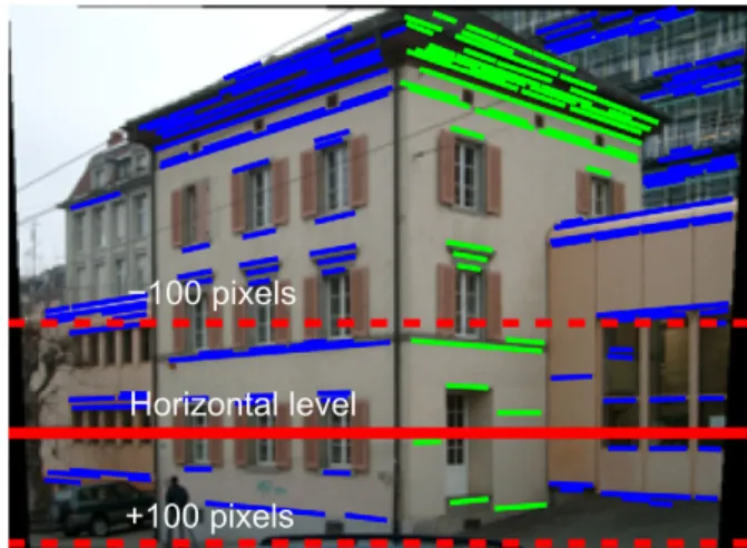
point with the highest voting score is chosen and its corresponding inlier lines are kept for further grouping. After dividing the entire collection of line segments into several small subsets, we can easily identify the true vanishing points and remove outliers. Moreover, we restrict the search of a possible vanishing point to a small hor-izontal strip by exploiting the fact that the ‘‘horizon’’ (the line con-necting the horizontal vanishing points) will appear horizontal in the tilt rectified image. We find a vanishing point with high voting score and use its row coordinate as the ‘‘horizon’’ level, as demon-strated inFig. 5. Only the candidates within a small horizontal strip
around the ‘‘horizon’’ level (±100 pixels) will be further verified, thus many false candidates can be immediately discarded. Finally, we simultaneously refine the results of line grouping and vanishing point estimation by applying the Expectation Maximization algo-rithm (EM)[20]. EM iteratively estimates the coordinates of vanish-ing points as well as the probability of an individual line segment belonging to a particular vanishing direction.
3.2.1. Performance evaluation
We tested the line grouping algorithm on the ZuBud building dataset[33]. The proposed method can generate good line group-ing results in urban environments. For all 1005 buildgroup-ing images, the algorithm can identify at least one principal direction and its associated parallel lines.Fig. 6shows some representative results of line grouping. It is noted the method can robustly identify par-allel building edges in the presence of a large amount of clutters as shown inFig. 6a. Also the method can successfully find a vanish-ing point for the lines on a minor plane (Fig. 6b) and can even han-dle some curved building facades by approximating them as piecewise-planar (Fig. 6c). The grouped line segments provide a basis for the following 3D reconstruction and viewpoint normali-zation procedures.
4. 3D planar reconstruction
After obtaining images of sets of parallel line segments, we pro-pose an effective method to divide a single monocular image into several vertical strips, with each strip corresponding to a 3D plane in the scene (e.g. a single facade of the building surface). The meth-od consists of two steps. First, we use the extracted vertical parallel lines to generate a number of 3D layout candidates. Then, each candidate is evaluated by referring to the distribution of parallel line segments from horizontal directions. The best fitting model is chosen to describe the 3D layout of the imaged scene.
Assuming buildings have vivid enough vertical boundaries, we use the vertical lines extracted on a tilt rectified image to generate 3D layout models in a cascade manner. First we choose the left-most and rightleft-most vertical lines to generate the simplest model containing one single dominant 3D plane. Then we select another vertical line and add it into an existing model to generate the mod-els containing two planes. By repeatedly adding more vertical lines into the existing structures, we can create models to describe scenes containing multiple 3D planes, as demonstrated inFig. 7.
The line segments from a horizontal vanishing direction provide a strong indication of the existence of a 3D plane in their direction. InFig. 8aLine 1defines a vertical strip which supports a 3D plane in its corresponding direction, whileLine 2suggests another plane in a different direction. After generating a number of 3D layout models based on the extracted vertical lines, we evaluate how well each one fits the collection of horizontal parallel line segments.
LetLxbe the candidate model which containsxplanes.
Accord-ingly the image will be divided into x vertical image strips S= {s1,s2,. . .,sx}. For a stripsk, the supporting score for it belonging
to the vanishing directionViis computed as:
j
ðVi;skÞ ¼ P lj2CðVi;skÞjljj P lj2CðskÞjljj ð8ÞwhereC(sk) is the set of line segments contained within the stripsk,
C(Vi,sk) is the set of lines belongs to the vanishing directionVi
with-in the stripsk, andjljjdenotes the length of a linelj. The directionVk
with the maximum supporting score will be assigned to the whole strip. Then the fitting score for this layout candidate is computed as:
KðLxÞ ¼ X sk2S
j
V k;sk AREAðskÞ ð9Þ 0 200 400 600 800 1000 1200 1400 1600 1800 2000 0 50 100 150 200 250 300 Number of images Focal LengthFig. 2.The distribution of the calculated focal lengths for 1005 images in the ZuBud dataset.
whereAREA(sk) is the area percentage of vertical stripskin the
im-age. The model which produces the highest fitting score will be cho-sen to describe the 3D layout of the imaged scene. In practice, if the fitting score does not increase significantly (0.1 in our implementa-tion) after adding more planes, we use the model of fewer planes to represent the 3D layout for better efficiency.Fig. 8b shows the final result of image segmentation, in which each color-coded vertical strip corresponds to a different 3D plane.
4.1. Performance evaluation
We have tested this method on 100 images selected from the ZuBuD building dataset[33]. We manually divided the images into several vertical strips and labeled the ground truth for each one. In total, 51 images have less than 10% misclassified pixels and 89 images have less than 20% misclassified pixels. On average, 84% of the image areas are correctly labeled using the proposed meth-od. Some example results are shown inFig. 9. Compared with some previously proposed monocular 3D recovery methods based on statistic learning [17,16]or high-level characterization [24,6,21], our approach is much simpler although it is capable of generating satisfactory 3D models of urban scenes. The output of our approach consists of a number of detected 3D planes which can be easily re-ferred to perform viewpoint normalization.
5. Viewpoint invariant features
Within each extracted image strip which corresponds to a 3D plane, we choose four line segments (two from the vertical direction
P11P12;P13P14 and two from a horizontal directionP11P14; P12P13)
and compute their points of intersection to construct a quadrilateral (P11,P12,P13,P14) (seeFig. 10). We then need to compute the
homog-raphy,H2R33, which relates the obtained quadrilateral in the 2D
image to a rectangle in the 3D world. Without loss of generality we assume that the four corners of a rectangle in the 3D world are denoted by homogeneous coordinates as follows:
X4 ¼ 0 0 sh sh 0 h h 0 0 0 0 0 1 1 1 1 2 6 6 6 4 3 7 7 7 5 ð10Þ
wherehis the height of a 3D rectangle andsis the ratio between its width and height, as explained inFig. 10. The mapping between 3D world positions and 2D image coordinates satisfies the following relations: x4’K½R1R2R3t X4 ¼K½R1R2t 0 0 sh sh 0 h h 0 1 1 1 1 2 6 4 3 7 5 ¼K½R1R2tdiagðsh;h;1Þ 0 0 1 1 0 1 1 0 1 1 1 1 2 6 4 3 7 5 ð11Þ 0 100 200 300 400 500 600 700 800 900 1000 0 1 2 3 4 5 6 7 8 9 10 Image index
Average x coordinate differences
Before tilt rectification After tilt rectification
Fig. 3.The average column coordinate differences between two endpoints of the vertical line segments for 1005 images in the ZuBud dataset. After tilt rectification, the differences decrease significantly. It means that the images of vertical building edges become much more parallel to the image columns.
Fig. 4.Some example results of camera tilt rectification. The vertical edges are highlighted to demonstrate the effect. The building boundary edges will appear vertical after the tilt rectification.
Horizontal level
+100 pixels
−100 pixels
Fig. 5.A demonstration of searching for the vanishing point along the horizontal level (the line connecting the horizontal vanishing points). Image coordinates of the two calculated orthogonal vanishing points are [587, 382, 1]Tand [1376, 396, 1]T, respectively.
DenoteHsthe transformation that maps the quadrilateral patch to a
unit square and substitute it into Eq.(11)to obtain:
Hs¼K½shR1hR2t ð12Þ
Since the image coordinates of the four corners of the quadrilateral are known,Hscan be solved in closed form. NoteR1andR2are
col-umns of a rotation matrix and should have unit normal, and hence the aspect ratioscan be recovered as follows:
s¼ H1 s H2s ð13Þ whereH1s andH 2
s are the first and second columns of matrixK1Hs.
Once the aspect ratio s is recovered, we compute the warping homographyHwarpwhich satisfies following relations:
x4¼Hwarp 0 0 shimg shimg 0 himg himg 0 1 1 1 1 2 6 4 3 7 5 ð14Þ
The value of heighthimgcontrols the size and the resolution of the
warped image. We determine its value based on the size of the se-lected quadrilateral as follows:
himg¼ P11P12 þ P13P14 2 ð15Þ
wherejP11P12jdenotes the length of a line segmentP11P12. In the
case where several rectangles are detected in an image (each one corresponding to a different 3D plane), we need to find a set of appropriate height ratios to make them have the same universal scale. Consider two quadrilateral (P11,P12,P13,P14) and
(P21,P22,P23,P24) detected in the image, we extend the horizontal
line segmentsP11P14;P12P13;P21P24;P22P23towards the intersection
line Lintersect between the two planes, as shown in Fig. 10. Then
the relative height ratio is given as:
h1img h2img ¼ P 0 11P 0 12 P0 21P 0 22 ð16Þ P0 11¼P11P14Lintersect;P012¼P12P13Lintersect P0 21¼P21P24Lintersect;P022¼P22P23Lintersect ð17Þ
The computed homography Hwarp enables us to warp the original
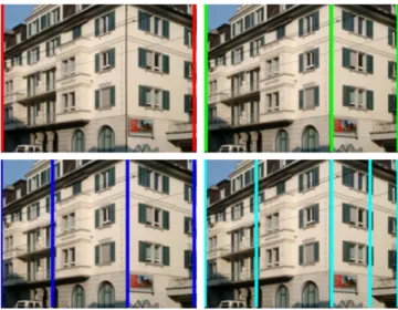
image of a 3D plane back to a normalized front-parallel view where the effects of 3D camera rotation and perspective are removed. Fig. 11 shows some examples of such viewpoint normalization. Obtaining the front-parallel view simplifies the task of recognizing the same surface from different viewpoints.
On the normalized front-parallel views of building facades, the viewpoint invariant features are computed in the same manner as the SIFT scheme [3]. Considering each side of a building can be Fig. 6.Example results of line grouping. The color coding corresponds to the membership assignment of the individual line segments.
Fig. 7.The process of generating multiple-plane 3D building layout candidates by adding more vertical lines into the existing models.
approximated by a 3D plane, feature extraction is efficiently per-formed in a single pass with respect to this plane. A complete view-point invariant feature consists of the following components: (1)x is its 2D coordinates in the original image; (2)x0is its 2D position in the normalized front-parallel view; (3)sis its corresponding spatial patch scale; (4)gis the dominant gradient orientation of the normalized patch; and (5) f is the 128-element descriptor. The proposed viewpoint invariant feature is similar to [9,10] in spirit, although our technique uses single images for both view-point normalization and feature extraction.
5.1. Effects of inaccurate focal length
To calculate the aspect ratiosin Eq.(13), we need to pre-mul-tiply the computed homography Hs by K1. In this section, we
investigate the influence of error in the estimated focal length on the performance of viewpoint normalization. Letf⁄denotes the cal-culated camera focal length, then we have
K1H s¼
a
shr11a
hr12a
txa
shr21a
hr22a
ty shr31 hr32 tz 2 6 4 3 7 5 ð18Þwhere therijis the (i,j)th element of the camera rotation matrix and
a
is the ratio between the true focal lengthftrueand the estimatedfocal lengthf⁄
. Note if
a
= 1(f⁄=ftrue), then the aspect ratiostruecan be correctly calculated as shown in Eq.(13). Since the none-zero pitch and roll angles have been compensated in the step of tilt rec-tification, we can approximate the rotation matrix of a tilt rectified image as follows: R cosw 0 sinw 0 1 0 sinw 0 cosw 2 6 4 3 7 5 ð19Þ
Substituting the elements of this matrix into Eq.(18)we obtain
K1 Hs
a
sh:cosw 0a
tx 0a
ha
ty sh:sinw 0 tz 2 6 4 3 7 5 ð20ÞThen the ratio between the estimated aspect ratios⁄
and the correct aspect ratiostrueis obtained as follows:
b¼ s strue¼ ffiffiffiffiffiffiffiffiffiffiffiffiffiffiffiffiffiffiffiffiffiffiffiffiffiffiffiffiffiffiffiffiffiffiffi
a
2cos2wþsin2 w qa
ð21ÞIt is noted that the ratiobis dependent on both the camera yaw an-gle
w
and the focal length ratioa
. We setw
= 0°, 30°, 45°, 60°(0° means the camera optical axis is normal to the building facade) and the range ofa
is from 0.1 to 10, then the value ofbis calculated and shown inFig. 12. It is noted that the estimation of aspect ratios is quite robust to small deviations of camera focal length. Forw
= 45°, when f⁄= 0.5ftrue (a
= 2) and 1.5ftrue (a
= 0.67), theestimated aspect ratio s⁄
= 0.7906strue (relative error is 10.7906 = 20.94%) and 1.2704strue (relative error is
1.27041 = 27.04%), respectively. InFig. 13, we show some results of viewpoint normalization using the pre-calculated focal lengths from the step of tilt rectification. As can be seen from the figure the appearances of a same building are quite consistent in two indi-vidually normalized views.
6. Performance evaluation
In this section we systematically evaluate the results of the pro-posed viewpoint normalization. We used the benchmark urban building image dataset – ZuBuD[33]. The dataset consists of multi-ple images covering 201 buildings in Zurich city center. For each building, five images were acquired at significantly varied view-points, in various seasons, and under different weather and illumi-nation conditions. Some of the images in ZuBuD dataset were taken using cameras rotated 90°in roll, so we pre-rotated them 90° re-versely before experiments.
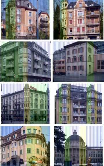
For the purpose of our experiments we selected 30 buildings1
from the ZuBuD dataset where, for each building, we used the two images taken over the widest baseline (the 1st and 5th views). These images contain dominant planar structures, therefore we can easily relate them via homography functions to facilitate quantitative eval-uations. Some representative images are shown inFig . 14, where significant viewpoint changes can be observed. For each image pair, a number of SIFT and viewpoint invariant features were extracted on the original images and on the normalized front-parallel views, respectively. Then, we followed the method described in[34]to de-fine a set of ground truth matches. The extracted features in the first image were projected onto the second one using the homography relating the images (we manually selected 4 well-conditioned corre-spondences to calculate the homography). A pair of features is con-sidered matched if the overlap error of their corresponding regions is minimal and less than a threshold[34]. We adjusted the threshold value to vary the number of resulting feature correspondences. 6.1. Similarity evaluation
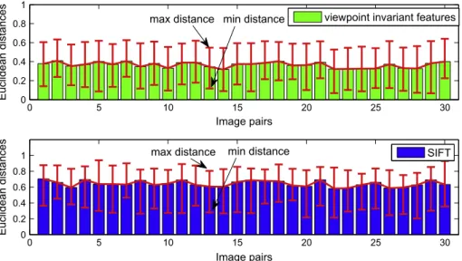
In the first experiment, we evaluate how well two correctly matched features relate with each other in terms of the Euclidean distance between their corresponding descriptors, their scale ratio, and their orientation difference. For each image pair, we selected 200 correspondences and calculated the average Euclidean dis-tance between their descriptors. The quantitative results are shown inFig. 15. It is noted from the results that the procedure of viewpoint normalization will compensate the effects of perspec-tive distortion and hence the resulting feature descriptors remain more invariant when viewpoint changes. This is evident in the fact that the average Euclidean distance between the matched features deceased significantly from 0.6432 (the average value for 30 image pairs) to 0.3651 after the procedure of viewpoint normalization.
For each pair of matched features, we also computed the differ-ence between their dominant orientations and the ratio between their patch scales. The results are shown inFigs. 16 and 17, respec-tively. On a normalized front-parallel view, the camera viewing direction is normal to the extracted 3D plane and the camera roll angle becomes zero. The matched features extracted on such nor-malized views should have the same dominant orientations and scale ratios. In experiments, it’s observed that the dominant Fig. 8.The line segments from horizontal vanishing directions provide important
cues for 3D understanding of the scene.
1Selected buildings: 0005, 0007, 0010, 0013, 0015, 0025, 0039, 0040, 0041, 0043, 0051, 0055, 0056, 0062, 0077, 0086, 0092, 0094, 0101, 0108, 0110, 0115, 0118, 0123, 0142, 0149, 0157, 0184, 0186, 0190.
orientations and scale ratios are equal up to a very small tolerance for all true correspondences after viewpoint normalization.
To qualitatively demonstrate the improvements, we show a number of matched viewpoint invariant features on the normal-ized images (seeFig. 18). Their corresponding scales and orienta-tions are also displayed. It can be clearly observed from these images that the matched viewpoint invariant features have similar orientations and consistent scale ratios. The results demonstrate that we can robustly make use of the scale and orientation infor-mation associated with local image features to generate geometric constrains between images. For viewpoint invariant features, a
single correspondence is enough to completely determine a homo-thetic function mapping two images. Using this simplified model, a much smaller number of samples are required to generate a correct hypothesis in the RANSAC iterations. Further efficiency evaluation results are provided in Section7.
6.2. Descriptiveness evaluation
Given a number of extracted image features, putative corre-spondences are usually established by searching the matches with minimum descriptor distances. In the second experiment, we dem-onstrate that the performance of this step can be improved using the viewpoint invariant features. To quantitatively evaluate the performances, the following data was obtained:
(1) Within a number of putative matches which have the closest descriptor distances –N1, we counted the number of correct
ones –N2.
(2) The ratio betweenN2andN1which provides the percentage
of correct correspondences in the putative set.
(3) The ratio between the closest Euclidean distance and the second closest one. We only computed this ratio for those correct correspondences.
The results are shown inFigs. 19–21, respectively. It is noted that the descriptiveness of local features is improved in twofold after the 3D viewpoint normalization. First, the putative match sets contain more correct correspondences (Fig. 19) and higher inlier percentages (Fig. 20). Therefore, more correct matches can be found by searching the minimum descriptor distances. Second, the gap between the closet distance and the second Fig. 9.Some examples of image segmentation. The color-coded vertical strips
correspond to 3D planes in different directions.
P
P
12P
P
11P’
11P’
P’
P
21 12 21 22P
24 23P’
P
14P
13 height1 height 2 22 width1 width2Fig. 10.Four line segments are chosen to construct a quadrilateral within each extracted vertical strip. In case multiple 3D planes exist, we need to find an appropriate height ratio to make them have the same universal scale.
Fig. 11.Some examples of viewpoint normalization. Note the perspective distortions are removed in the warped front-parallel views of the building walls (e.g. a rectangular window in the 3D world will also appear rectangular in the normalized image). In case multiple planes are detected within the image, we set an appropriate height ratio to make them have the same universal scale.
closet one becomes wider (Fig. 21). It means that the best match candidate significantly outperforms the second best one, thus it is easy to identify a distinctive match. These improvements enable us to establish robust matches over widely separated views.
7. Wide baseline matching in urban environments
In this section we propose an effective framework for robust wide baseline image matching in urban environments using the extracted viewpoint invariant features. Given two images of an ur-ban scene captured from widely separated viewpoints, which may contain considerable repetitive structures (e.g. windows), our objective is to establish robust feature correspondences between
them. This represents a challenging problem for two reasons. First, the same building facade will appear very different when the cam-era viewpoint is changed significantly. Using descriptors directly computed on such wide baseline images, it is difficult to establish correct matches. Second, man-made buildings usually contain many structures of similar appearances. This can result in consid-erable aliasing in the matching process. For example, it may be possible to match any single window in the first image with any window in the second one based on comparing local appearances. Hence any solution to the above problem must be invariant to the distortions introduced by the imaging process and be robust to ali-asing within the scene.
We follow the commonly used image matching scheme of: (1) establishing a set of putative correspondences based on matching
−1 0 1 0 0.5 1 1.5 2 log 10α β 0 degree −1 0 1 0 2 4 6 log 10α β 30 degree −1 0 1 0 2 4 6 8 log 10α β 45 degree −1 0 1 0 5 10 log 10α β 60 degree
Fig. 12.The effect of uncalibrated camera focal length.ais the ratio between the ground truthftrueand an arbitrarily selected focal lengthf⁄.bis the ratio between the estimated aspect ratios⁄
and the correct aspect ratiostrue.
Fig. 13.Some results of viewpoint normalization using the focal lengths calculated in the step of tilt rectification. It is observed the appearances of the same building are quite consistent in two individually normalized views.
Fig. 14.Example image pairs used for performance evaluations. These images all contain dominant planar structures, therefore we can easily relate them through a homography function to facilitate quantitative experiments.
local descriptors, and (2) computing a global geometric constraint to identify true correspondences across the views. Given a number of extracted viewpoint invariant features, we first establish a set of putative correspondences based on matching local descriptors. In [3]a pair of features are considered matched if the ratio between distances to the closest match and to the second closest is below some predefined threshold. The ratio check scheme is justified be-cause the correct match for a discriminative keypiont is often sig-nificantly better (closer in the descriptor space) than the incorrect ones[3]. However, in urban environments where many repetitive structures (e.g. windows) exist, this criterion will falsely reject correct matches since a feature cannot find a unique distinctive match. In our proposed framework we accept multiple matches to cope with repetitive urban structures. Two features are consid-ered matched if the cosine of the angle between their descriptorsfi
andfjis above some thresholddas[35]:
cosðfi;fjÞ ¼
fT
i :fj
kfik2kfjk2
>d ð22Þ
where kk2 represents the L2-norm of a vector. In case multiple
matches meet the criterion, we keep the top 10 matches for further verification. In urban environments where many repetitive struc-tures (e.g. windows) exist, this criterion establishes matches be-tween features having similar descriptors. This keeps the potential correspondences extracted on the images of repetitive structures for further geometric verification. After the tilt rectification (the viewing direction is parallel to the ground plane and the camera roll angle becomes zero) and the viewpoint normalization (camera changes to a front-parallel view), the matched features will have very similar gradient orientations (seeFig. 16). If the orientation dif-ference between a pair of matched features is above some threshold (5°in our implementation), the match is considered as an outlier and removed from the putative set. However, Eq. (22)is a quite loose criterion. The resulting putative set will contain a large per-centage of outliers (90–95%), within which we need to identify the correct correspondences.
After obtaining a set of putative feature matches based on the matching of local descriptors, we need to refine the results and
0 5 10 15 20 25 30 0 20 40 60 80 Image pairs orientation differences
max difference min difference SIFT
0 5 10 15 20 25 30 0 20 40 60 80 Image pairs orientation differences
max difference min difference
viewpoint invariant features
Fig. 16.The average orientation differences between matched features for 30 selected image pairs. It is noted that the matched viewpoint invariant features have very similar dominant orientations, and the average orientation difference is 3.17°(the average for 30 image pairs). In comparison, the average orientation difference of the matched SIFT features is 23.84°. 0 5 10 15 20 25 30 0 0.2 0.4 0.6 0.8 1 Image pairs Euclidean distances
max distance min distance viewpoint invariant features
0 5 10 15 20 25 30 0 0.2 0.4 0.6 0.8 1 Image pairs Euclidean distances
max distance min distance SIFT
Fig. 15.The average Euclidean distances between the descriptors of matched features. For 30 image pairs, the average Euclidean distance between the matched features deceased from 0.6432 to 0.3651 after the procedure of viewpoint normalization. Hence the matched features extracted on the normalized front-parallel views have more similar descriptors.
to identify the true correspondences by imposing a geometric con-straint. The RANSAC technique[29]is usually applied for this task. The essence of the RANSAC algorithm is the generation of multiple hypotheses by iteratively sampling the data and the verification of each one by computing its corresponding supports. The number of samplesMrequired to guarantee a confidence
q
that at least one sample is outlier free is computed as:M¼ lnð1
q
Þlnð1 ð1
ÞPÞ ð23Þwhere
is the percentage of outliers andPis the number of obser-vations required to generate a hypothesis per sample (in this case it is the number of feature correspondences needed to compute the H-matrix or F-H-matrix). As shown inTable 1, when the fraction of out-liers is significant and the geometric model is complex, RANSAC needs a large number of samples and becomes prohibitively expen-sive. Since the effects of perspective transformation are not com-pensated in the standard 2D feature schemes (e.g. SIFT), only the2D image coordinates of extracted features can be used to generate geometric constraints (e.g. F-Matrix or H-Matrix). Therefore, a num-ber of SIFT feature matches are required to compute the F-Matrix (7 correspondences) or the H-matrix (4 correspondences). In compar-ison, viewpoint invariant features contain enough information (i.e.x andycoordinates, scale ratio, and orientation) to define a homo-thetic constraint given a single feature correspondence as follows:
x01¼ s1=s2 0
D
x 0 s1=s2D
y 0 0 1 2 6 4 3 7 5x02 ð24Þwherex01and x02 are the 2D feature positions in the normalized front-parallel views,s1ands2are their corresponding patch scales.
As shown inFigs. 16–18, the scale and orientation information asso-ciated with local image features is robust enough to generate geo-metric constrains between images. Using this simple geogeo-metric model, a much smaller number of samples are needed to guarantee the generation of a correct hypothesis.
0 5 10 15 20 25 30 0 1 2 3 Image pairs Scale ratios
max ratio min ratio SIFT
0 5 10 15 20 25 30 0 1 2 3 Image pairs Scale ratios
max ratio min ratio
viewpoint invariant features
Fig. 17.The average scale ratios between matched features with the maximum and minimum annotated. It is shown that the matched viewpoint invariant features have very consistent scale ratio. Given a single correctly matched features, the scale factor between two images can be robustly determined.
To demonstrate such improvements an experiment was carried out where we selected 200 ground truth correspondences to set up the initial putative set. For each iteration of the experiment we in-creased the number of false feature matches (outliers) into the putative set and used the RANSAC algorithm to identify the inliers. We set the maximum sampling number at 10000 and confidence parameter
q
at 0.95. For each putative set (30 sets in total) we run RANSAC for 10 times and compute the average sampling num-ber. The results of this procedure are shown inTable 2. Here we have implemented a H-constraint for SIFT, whereas for the view-point invariant features, we used the geometric constraint de-scribed in Eq.(24).It is noted that the required number for RANSAC iterations de-creased significantly due to the use of the simplified geometric model. Moreover, RANSAC can successfully return the true corre-spondences from a putative feature set containing a high percent-age of outliers. As shown inTable 2, the true correspondences can be identified from a putative set containing 98% outliers within a few hundred iterations. This is an important observation. It means
we can set a weak criterion (Eq.(22)) to establish a large number of putative matches (i.e. containing a large number of outliers) and then effectively impose the simplified geometric constraint de-scribed in Eq.(24)to identify the correct ones. However, this can-not be achieved using the standard SIFT features since only the 2D feature coordinates can be used to generate geometric constraints (F-Matrix or H-Matrix). If the putative set contains a high percent-age of outliers (more than 80%), RANSAC needs a large number of iterations to return the true correspondences (see the required sampling number using SIFT inTable 2).
7.1. Experiments
First we quantitatively evaluate our proposed scheme for fea-ture matching across variable view angles. We used the image se-quence covering the 0016 building in the ZuBuD dataset (see Fig. 22) for this task. The first image was chosen as the reference frame and the other images were matched against it. The other fea-ture schemes we compared included SIFT[3], Harris-Affine[4,34],
0 5 10 15 20 25 30 0 500 1000 1500 2000 Image pairs Number of matches N
1 − viewpoint invariant features N
2 − viewpoint invariant features
0 5 10 15 20 25 30 0 500 1000 1500 2000 Image pairs Number of matches N 1 − SIFT N 2 − SIFT
Fig. 19.For a number of putative correspondences which have the minimum descriptor distancesN1, we counted the number of correct onesN2. Using viewpoint invariant features, more correct matches can be found in the resulting putative set.
0 5 10 15 20 25 30 0 0.1 0.2 0.3 0.4 0.5 Image pairs Inlier percentage
viewpoint invariant features
0 5 10 15 20 25 30 0 0.1 0.2 0.3 0.4 0.5 Image pairs Inlier percentage SIFT
Fig. 20.Inlier percentages in the putative sets given by the ratio between the number of correct matches (N2) and the number of putative matches (N1). The average inlier percentage of 30 selected image pairs increased from 15.29% to 25.52% after the procedure of viewpoint normalization.
Hessian-Affine [34], Maximally Stable Extremal Regions (MSER) [1], Edge Based Region (EBR) [5], and Intensity Based Region (IBR)[5]. The features were individually extracted on each single image and their characteristics were described using the 128-vec-tor SIFT descrip128-vec-tor. A number of putative matches were initially established by following the criterion described in Eq. (22) (d was set at 0.9). Then the inlier correspondences were automatically identified by using the RANSAC technique. For the viewpoint invariant features, we implemented the homothetic mapping con-straint described in Eq.(24). For other feature schemes, we imple-mented the H-matrix mapping constraint. The final correct matches were manually counted and the results are summarized inFig. 23.
Using the features extracted on the normalized front parallel views, a good number of correct feature matches can still be found under significant view angle changes (between the 1st and 5th views). It is noted that the number of matches dropped
signifi-cantly when the viewpoint was changed from the 2nd image to the 3rd image. This is because a large area of the reference frame (the 1st image) is not covered in the 3rd image. The second best feature detector is SIFT. Other detectors either fail or find a very small number of matches between the images taken from different viewpoints.
Next we demonstrate the advantages of the proposed feature matching scheme by applying it to some difficult wide baseline matching tasks. We tested the proposed method on the 1st and the 5th views of buildings contained in the ZuBuD dataset, which have the largest viewpoint changes (in many cases the view angles changed more than 90°). We first found a number of putative cor-respondences based on Eq.(22)(the thresholddwas set at 0.9).
0 5 10 15 20 25 30 0 0.5 1 1.5 Image pairs Distance ratio
viewpoint invariant features
0 5 10 15 20 25 30 0 0.5 1 1.5 Image pairs Distance ratio SIFT
Fig. 21.The average ratio between the closest distance and the second closest one. Low distance ratio means the best match is significantly better than the second best one, thus a distinctive match can be easily found for a feature. The average distance ratio is 0.7948 for the standard SIFT features, in comparison the ratio decreases to 0.6624 using the viewpoint invariant features.
Table 1
The theoretical number of samples required for RANSAC to ensure 95% confidence that one outlier free sample is obtained for the geometric constraint estimation. The actual required number is around an order of magnitude more.
Outlier ratio 40% 50% 60% 70% 80%
Our method (1 point) 4 5 6 9 14
H-matrix (4 point) 22 47 116 369 1871
F-matrix (7 point) 106 382 1827 13696 234041
Table 2
The experimental number of trials to ensure RANSAC selects, with 95% confidence, an outlier free sample for the geometric constraint estimation. It is noted that the required sample number decreased significantly using viewpoint invariant features. Moreover, RANSAC can successfully return the true correspondences from a putative feature set of high outlier percentage (98% outliers contained). This is particularly advantageous for image matching in urban environments where lots of respective structures (e.g. windows, doors, bricks) exist.
Outlier ratio Viewpoint invariant features SIFT
40% (133 outliers) 5.5 44.2 60% (300 outliers) 9.4 155.8 80% (800 outliers) 22.4 2309.8 90% (1800 outliers) 37.6 > 10000 95% (3800 outliers) 74.8 > 10000 98% (9800 outliers) 212.2 > 10000 Table 3
The quantitative results of wide baseline matching, corresponding to the images in Fig. 24. (M1/M2 – the numbers of extracted features on image 1 and 2 respectively, P – the number of putative correspondences, I – the number of inlier correspondences returned by the RANSAC technique, C – the number of correct ones). Using SIFT features we need to make sure the resulting putative sets have a good portion of inliers (more than 20%), otherwise RANSAC can’t return the correct correspondences after reaching the maximum number of iterations. Setting a strict criterion will sacrifice a large number of true correspondences (see the numbers of generated putative matches for comparison).
Image pairs SIFT Viewpoint invariant features
a 993(M1)/1009(M2) 1401(M1)/1321(M2) 15(C)/33(I)/118(P) 125(C)/125(I)/2313(P) b 1228(M1)/1308(M2) 1007(M1)/1198(M2) 3(C)/22(I)/124(P) 122(C)/126(I)/1954(P) c 2021(M1)/2629(M2) 2502(M1)/3433(M2) 0(C)/35(I)/223(P) 64(C)/64(I)/1378(P) d 1936(M1)/3223(M2) 2721(M1)/3090(M2) 0(C)/26(I)/135(P) 46(C)/48(I)/1381(P) e 2595(M1)/2540(M2) 3241(M1)/2841(M2) 15(C)/22(I)/180(P) 298(C)/298(I)/2342(P) f 3282(M1)/3064(M2) 3501(M1)/2972(M2) 4(C)/59(I)/320(P) 103(C)/104(I)/1894(P) g 2830(M1)/1698(M2) 2910(M1)/2508(M2) 0(C)/21(I)/139(P) 98(C)/98(I)/2421(P) h 4266(M1)/3198(M2) 4610(M1)/4111(M2) 0(C)/18(I)/194(P) 81(C)/89(I)/1711(P) i 1974(M1)/1295(M2) 1810(M1)/1405(M2) 11(C)/26(I)/211(P) 54(C)/59(I)/1525(P)
Then we removed outliers by checking the orientation differences. Finally we applied the RANSAC algorithm to impose the constraint described in Eq.(24)to identify inliers. The number of inlier corre-spondences and correct ones were counted manually. For compar-ison, we applied the SIFT feature scheme to the same image pairs. A set of putative matches were firstly established. In this step, we need to set a strict criterion to make the resulting putative sets have a good portion of inliers (more than 20%), otherwise RANSAC typically fails to return the correct correspondences after reaching the maximum number of samplings (seeTable 2). In experiments, we applied the ratio check scheme[3]and set the ratio threshold at 0.85. Setting a strict matching criterion (ratio check[3]) will ini-tially sacrifice many true correspondences (see the numbers of generated putative matches inTable 3for comparison). Then we used RANSAC to compute the correct H-matrix to identify inlier correspondences.
Out of 201 buildings, we get 185 (92.04%) good matching re-sults (more than 20 correct matches can be identified) using the Fig. 22.The image sequence of the0016building in the ZuBuD dataset. Images were taken of the same building from changed viewpoints.
2 3 4 5 0 100 200 300 400 500
Viewpoint invariant features SIFT EBR Haraff Hesaff IBR MSER Number of correct matches
Matched image
Fig. 23.The performance of various feature techniques for image matching over variable viewpoint changes.
(a)
(b)
(c)
(d)
(e)
(f)
(g)
(h)
(i)
Fig. 24.Some example results of wide baseline feature matching. Significant viewpoint changes can be observed in the image pairs. (The left column shows the results of using SIFT and the right column is the results of using our proposed viewpoint invariant features). Using viewpoint invariant features we are able to establish correct matches over widely separated images and to cope with repetitive structures in urban environments.
viewpoint invariant features. In comparison, we only get 127 good matching results (62.87%) using SIFT. Some representative match-ing results are shown inFig. 24with the quantitative results pro-vided in Table 3. It is noted that SIFT features only work well when the viewpoint separation between two image centers is rel-atively small compared to the distance between the camera and the observed object (e.g. building 0161–0171 where images were captured at a distant position, thus the appearance of a building would not change too much when camera viewpoint is slightly moved).
In total, there are 16 failed cases.2Some examples are given in Fig. 25. Building facades sometimes are blocked by foreground ob-jects such as trees, signs, people, and other clutters in urban environ-ments. When the blockage is significant, appearance-based feature technique will fail to identify correct image correspondences, as shown inFig. 25a. Another reason for failure is that when camera viewpoint is significantly changed, a dominant planar structure in the first image might appear in a small region in the second view, as shown inFig. 25b. In these cases viewpoint invariant features can-not produce satisfactory matching results.
To summarize, the proposed viewpoint invariant feature achieves a two-fold improvement in terms of wide baseline match-ing in urban environments. First, the procedure of viewpoint nor-malization will compensate for the effects of perspective distortion to ensure the resulting feature descriptors remain more invariant when viewpoint changes, as shown inFig. 15. Using the improved local descriptors we can establish correct correspon-dences over widely separated images. Second, the scale and orien-tation information associated with viewpoint invariant features can be robustly used for effective geometric verification (see Figs. 16 and 17) to deal with visual aliasing in urban scenes. This makes viewpoint invariant features particularly suitable for image matching in urban environments where lots of repetitive struc-tures exist.
8. Conclusions
In this paper we proposed an effective method for extracting and matching viewpoint invariant features from single images. The key idea is to use the 3D geometry as an additional cue to im-prove the performance of 2D features. Given an image taken in ur-ban environments, we present an effective method to recover its 3D layout from the extracted line segments. Then the viewpoint invariant features are extracted on the normalized front-parallel views of 3D building facades. In this work we systematically eval-uated the performance of this novel feature. First, it is very robust against perspective distortions and viewpoint changes. Second, it contains robust local patch information (e.g. scale, orientation)
which enable efficient feature matching. Compared with some pre-vious works on combining 2D feature with 3D geometry, our meth-od works completely on single images and hence is more widely applicable. We have demonstrated the suitability of these novel features in the context of wide baseline matching tasks. In the fu-ture, we will further extend the method for images taken in more complex and larger scale environments. Eventually the method will be used as an important component in applications such as user navigation, augmented reality, and intelligent robotics in ur-ban environments.
Acknowledgments
Research presented in this paper was funded by a Strategic Research Cluster grant (07/SRC/I1168) by Science Foundation Ireland under the National Development Plan. The authors grate-fully acknowledge this support. The authors would also like to thank the reviewers for their valuable comments and suggestions. References
[1] M. Donoser, H. Bischof, Efficient maximally stable extremal region (MSER) tracking, IEEE Conf. Comput. Vision Pattern Recog. (2006) 553–560. [2] H. Bay, A. Ess, T. Tuytelaars, L. Van Gool, Speeded-up robust features (SURF),
Comput. Vis. Image Underst. 110 (3) (2008) 346–359.
[3] D.G. Lowe, Distinctive image features from scale-invariant keypoints, Int. J. Comput. Vision 60 (2) (2004) 91–110.
[4] T. Lindeberg, Feature detection with automatic scale selection, Int. J. Comput. Vision 30 (1998) 79–116.
[5] T. Tuytelaars, L. Van Gool, Matching widely separated views based on affine invariant regions, Int. J. Comput. Vision 59 (1) (2004) 61–85.
[6] B. Micusik, H. Wildenauer, J. Kosecka, Detection and matching of rectilinear structures, IEEE Conf. Comput. Vision Pattern Recog. (2008) 1–7.
[7] K. Mikolajczyk, T. Tuytelaars, C. Schmid, A. Zisserman, J. Matas, F. Schaffalitzky, T. Kadir, L. Van Gool, A comparison of affine region detectors, Int. J. Comput. Vision 65 (1–2) (2005) 43–72.
[8] J.-M. Morel, G. Yu, Asift: a new framework for fully affine invariant image comparison, SIAM J. Img. Sci. 2 (2009) 438–469.
[9] K. Koeser, R. Koch, Perspectively invariant normal features, IEEE Int. Conf. Comput. Vision (2007) 1–8.
[10] C. Wu, B. Clipp, X. Li, J. Frahm, M. Pollefeys, 3D model matching with viewpoint-invariant patches (VIP), IEEE Conf. Comput. Vision Pattern Recog. (2008) 1–8.
[11] K. Mikolajczyk, C. Schmid, A performance evaluation of local descriptors, IEEE Trans. Pattern Anal. Mach. Intell. 27 (10) (2005) 1615–1630.
[12] A. Zaharescu, E. Boyer, K. Varanasi, R.P. Horaud, Surface feature detection and description with applications to mesh matching, IEEE Conf. Comput. Vision Pattern Recog. (2009) 373–380.
[13] D. Robertsone, R. Cipolla, An image-based system for urban navigation, BMVC04 (2004) 819–828.
[14] H. Jegou, M. Douze, C. Schmid, Hamming embedding and weak geometric consistency for large scale image search, ECCV08 I (2008) 304–317. [15] D. Hoiem, A.A. Efros, M. Hebert, Automatic photo pop-up, ACM SIGGRAPH
(2005) 577–584.
[16] D. Hoiem, A.A. Efros, M. Hebert, Geometric context from a single image, IEEE International Conf. Comput. Vision (2005) 654–661.
[17] H. Derek, A.A. Efros, M. Hebert, Putting objects in perspective, IEEE Conf. Comput. Vision Pattern Recog. (2006) 3–15.
[18] V. Hedau, D. Hoiem, D. Forsyth, Recovering the spatial layout of cluttered rooms, IEEE Conf. Comput. Vision Pattern Recog. (2009) 1849–1856. Fig. 25.Some failed matching results. (a) A large portion of building facade is blocked, thus appearance-based feature techniques cannot find correct correspondences. (b) Due to significant viewpoint change a dominant plane in the first image only appears in a small area of the second view.
2
Failed cases: buildings 0002, 0003, 0006, 0017, 0018, 0058, 0098, 0107, 0109, 0112, 0114, 0119, 0121, 0122, 0199, 0200.
[19] A. Saxena, S.H. Chung, A.Y. Ng, 3-D depth reconstruction from a single still image, Int. J. Comput. Vision 76 (1) (2008) 53–69.
[20] J. Kosecka, W. Zhang, Video compass, ECCV (2002) 476–490.
[21] J. Kosecka, W. Zhang, Extraction, matching, and pose recovery based on dominant rectangular structures, Comput. Vision Image Underst. 100 (3) (2005) 274–293.
[22] Z. Zhang, A flexible new technique for camera calibration, IEEE Trans. Pattern Anal. Mach. Intell. 22 (11) (2000) 1330–1334.
[23] G. Wang, Z. Hu, F. Wu, H.-T. Tsui, Single view metrology from scene constraints, Image Vision Comput. 23 (9) (2005) 831–840.
[24] A. Criminisi, I. Reid, A. Zisserman, Single view metrology, Int. J. Comput. Vision 40 (2) (2000) 123–148.
[25] Z. Li, J. Liu, X. Tang, Shape from regularities for interactive 3d reconstruction of piecewise planar objects from single images, Multimedia (2006) 85–88. [26] O. Barinova, V. Konushin, A. Yakubenko, K. Lee, H. Lim, A. Konushin, Fast
automatic single-view 3-D reconstruction of urban scenes, ECCV (2008) 100– 113.
[27] Y. Cao, J. McDonald, Viewpoint invariant features from single images using 3D geometry, WACV09 (2009) 1–6.
[28] C. Rother, A new approach for vanishing point detection in architectural environments, BMVC (2000) 382–391.
[29] M. Fischler, R. Bolles, Random sample consensus: a paradigm for model fitting with applications to image analysis and automated cartography, CACM 24 (6) (1981) 381–395.
[30] R. Hartley, A. Zisserman, Multiple View Geometry in Computer Vision, Cambridge University Press, New York, NY, USA, 2003.
[31] G. Simon, A.W. Fitzgibbon, A. Zisserman, Markerless tracking using planar structures in the scene, Int. Symp. Augmen. Reality (2000) 120–128. [32] M. Pollefeys, R. Koch, L.V. Gool, Self-calibration and metric reconstruction
inspite of varying and unknown intrinsic camera parameters, Int. J. Comput. Vision 32 (1999) 7–25.
[33] T.S.H. Shao, L. Van Gool, Zubud-zurich buildings database for image based recognition, Tech. Rep. 260, Swiss Federal Institute of Technology, 2004. [34] K. Mikolajczyk, C. Schmid, Scale and affine invariant interest point detectors,
IJCV 60 (1) (2004) 63–86.
[35] W. Zhang, J. Košecká, Hierarchical building recognition, Image Vision Comput. 25 (5) (2007) 704–716.