Kernel methods for Monte Carlo

Heiko Strathmann

A dissertation submitted in partial fulfillment of the requirements for the degree of

Doctor of Philosophy of

University College London.

Gatsby Unit for Computational Neuroscience and Machine Learning University College London

I, Heiko Strathmann, confirm that the work presented in this thesis, except as noted herein, is my own. Where information has been derived from other sources, I confirm that this has been indicated in the work.

This thesis investigates the use of reproducing kernel Hilbert spaces (RKHS) in the context of Monte Carlo algorithms. The work proceeds in three main themes.

Adaptive Monte Carlo proposals

We introduce and study two adaptive Markov chain Monte Carlo (MCMC) algorithms to sample from target distributions with non-linear support and intractable gradients. Our algorithms, generalisations of random walk Metropolis and Hamiltonian Monte Carlo, adaptively learn local covari-ance and gradient structure respectively, by modelling past samples in an RKHS. We further show how to embed these methods into the sequential Monte Carlo framework.

Efficient and principled score estimation

We propose methods for fitting an RKHS exponential family model that work by fitting the gradient of the log density, the score, thus avoiding the need to compute a normalization constant. While the problem is of general interest, here we focus on its embedding into the adaptive MCMC context from above. We improve the computational efficiency of an earlier solution with two novel fast approximation schemes without guarantees, and a low-rank, Nyström-like solution. The latter retains the consistency and convergence rates of the exact solution, at lower computational cost.

Goodness-of-fit testing

We propose a non-parametric statistical test for goodness-of-fit. The mea-sure is a divergence constructed via Stein’s method using functions from an RKHS. We derive a statistical test, both for i.i.d. and non-i.i.d. samples, and apply the test to quantifying convergence of approximate MCMC methods, statistical model criticism, and evaluating accuracy in non-parametric score estimation.

I would like to express my deepest gratitude to my family, my supervisor Arthur Gretton, and the Gatsby unit.

1 Introduction 11

1.1 Overview . . . 11

1.2 Publications . . . 12

1.3 Motivation, contribution, and related work . . . 13

2 Background 25 2.1 Reproducing kernel Hilbert spaces . . . 25

2.2 Score matching & un-normalised density estimation . . . 29

2.3 Markov chain Monte Carlo . . . 32

I

Adaptive Monte Carlo proposals

35

3.2 MCMC Kameleon algorithm . . . 42

3.3 Experiments . . . 49

4 Gradient-free HMC with efficient kernel exponential families 59 4.1 Kernel Hamiltonian dynamics . . . 63

4.2 Two estimators for kernel exponential families . . . 64

4.3 Kernel Hamiltonian Monte Carlo . . . 69

4.4 Experiments . . . 71

4.5 Details for lite estimator . . . 82

5 Kernel sequential Monte Carlo 93

5.1 Sequential Monte Carlo . . . 94

5.2 Kernel sequential Monte Carlo . . . 99

5.3 Experiments . . . 102

II

Efficient and principled score estimation

111

6.2 Theory . . . 118

6.3 Experiments . . . 121

7 Proofs 127 7.1 Preliminaries . . . 127

7.2 Representer theorem for Nyström . . . 133

7.3 Consistency and convergence rates . . . 136

7.4 Auxiliary results . . . 144

III

Goodness-of-fit testing

155

8.2 Proofs of the main results . . . 162

8.3 Experiments . . . 167

IV

Conclusions

177

Introduction

1.1

Overview

This thesis explores how kernel methods can be used within the wider context of Monte Carlo, a method to solve integration problems, such as Bayesian expectations, using random samples. More specifically, we are concerned with the problems of efficient random sampling, learning struc-ture of unknown densities from data, and measuring how well a set of samples (e.g. obtained from a random sampling algorithm) fits a particular model.

The efficiency of Monte Carlo sampling algorithms, such as Markov chain Monte Carlo (MCMC), crucially relies on the proposal mechanisms that guide how the next step in the Markov chain trajectory is generated. We show how to construct a number of such proposal mechanisms via using kernel methods to model the structure of the underlying density, e.g. covariance or gradients. This results in a flexible framework that can be embedded into MCMC and sequential Monte Carlo algorithms.

The main ingredient for the above ideas is non-parametric modelling of the structure of an unknown probability density. Kernel methods pro-vide an elegant and computationally efficient framework for such mod-elling tasks, however, in practice they often come with considerable com-putational costs. In order to ensure practicality of such models in the

Monte Carlo context, we develop novel approximation schemes for existing kernel-based density models. Crucially, we develop statistical guarantees that trade-off introduced error with reduced computational cost.

Finally, the accuracy of Monte Carlo methods strongly depends on the ‘quality’ of the generated samples, often in the form of bias-variance trade-offs. This is for example the case in the approximate MCMC framework, where the variance of an estimator is reduced at the cost of introducing a (usually small) systematic error. We study how to measure sample quality in this context and develop a non-parametric goodness-of-fit test for non i.i.d. data, which can be used to tune such trade-offs systematically.

1.2

Publications

The thesis structure is based on the following publications. Each chapter is based on collaborative work with the co-authors as outlined in the chapters’ beginnings.

Adaptive Monte Carlo proposals

• D. Sejdinovic, H. Strathmann, M. Lomeli, C. Andrieu, and A. Gretton. “Kernel Adaptive Metropolis-Hastings”. In: International Conference for Machine Learning. 2012

• H. Strathmann, D. Sejdinovic, S. Livingstone, Z. Szabo, and A. Gret-ton. “Gradient-free Hamiltonian Monte Carlo with Efficient Kernel Exponential Families”. In: Advances in Neural Information Processing Systems. 2015

• I. Schuster, H. Strathmann, B. Paige, and D. Sejdinovic. “Kernel Adaptive Sequential Monte Carlo”. In: European conference on machine learning & principles and practice of knowledge discovery in databases. Joint first two authors. 2017

• D. Sutherland, H. Strathmann, M. Arbel, and A. Gretton. “Efficient and principled score estimation”. In: arXiv preprint arXiv:1705.08360

(2017). Joint first two authors. Submitted. Goodness-of-fit testing

• K. Chwialkowski, H. Strathmann, and A. Gretton. “A kernel test of goodness of fit”. In: International Conference for Machine Learning. 2016

1.3

Motivation, contribution, and related work

This section provides a brief introduction to the three main themes of this thesis, motivates the research objectives, and points out related work.

1.3.1

Adaptive Monte Carlo proposals

Estimating expectations using Markov Chain Monte Carlo is a fundamen-tal approximate inference technique in Bayesian statistics. Simply speaking, MCMC is a strategy for generating a Markov chain, a sequence of random samples X1,X2, . . . from potentially complex and high-dimensional

distri-butions π in a space X, where Xt+1 depends only on Xt. Using those samples, expectations can be estimated as

Z X f(x)π(x)dx≈ 1 n n

∑

given certain properties of the Xi, and π-integrable f, [6]. For example f(x) =xyields the mean ofπ.

The key building-block of the MCMC algorithms that we consider here is the Metropolis-Hastings algorithm, an algorithm that given a state Xt produces a proposal for Xt+1, and accepts or rejects it at random with a

probability that is based on the underlying density π. Since the expected estimation error in (1.1) directly depends on the correlation between suc-cessive points in the Markov chain [93], efficiency can be achieved by taking steps with little correlation (i.e. large) that are accepted with high probabil-ity. Proposal mechanisms that adapt to the target on the fly aim to strike

this balance. Care has to be taken though – using the Markov chain history to inform future moves generally compromises convergence properties of the resulting MCMC algorithm [6].

We will generally assume that the target density π is only available point-wise (in closed form or via a random estimator without bias), and no higher order information, such as gradients, is available. For example, in pseudo-marginal MCMC [5, 16], the target density does not have an analytically tractable expression, but can only be estimated at any given point, e.g. Bayesian Gaussian process classification [44]. A related setting is MCMC for approximate Bayesian computation (ABC), where a Bayesian posterior is approximated through repeated simulation from its likelihood [80, 108]. In those cases, sophisticated gradient-based schemes [50, 95] cannot be applied directly on the intractable target.

Kernel adaptive Metropolis-Hastings

The choice of the proposal distribution is known to be crucial for the design of Metropolis-Hastings algorithms, and methods for adapting the proposal distribution to increase the sampler’s efficiency based on the history of the Markov chain have been widely studied [6, 60, 61]. These methods often aim to learn the global covariance structure of the target distribution, and adapt the proposal accordingly.

Contribution.We develop a kernel adaptive Metropolis-Hastings algo-rithm (KAMH) in which the Markov chain trajectory is mapped to an RKHS, and the proposal distribution is chosen according to the covari-ance in this feature space [8, 110]. Unlike earlier adaptive approaches, the resulting proposals are locally adaptive in the input space, and oriented towards nearby regions of high density, rather than simply matching the global covariance structure of the distribution. Our approach combines a move in the feature space with a stochastic step towards the nearest input space point, where the feature space move can be analytically integrated out. Thus, the implementation of the procedure is straightforward: the

proposal is simply a Gaussian in the input space, with location-dependent covariance that is informed by the feature space representation of the tar-get. Furthermore, the resulting sampler only requires the ability to evaluate the un-normalised density of the target.

Related work.Adaptive MCMC samplers were first studied by Haario et al. [60, 61], who proposed to update the proposal along the sampling process. Based on the chain history, they estimate the covariance of the target distri-bution and construct a Gaussian proposal centred at the current chain state, with a particular choice of the scaling factor from [48]. More sophisticated schemes are presented by Andrieu and Thoms [6], e.g. adaptive scaling, component-wise scaling, and principal component updates. While these strategies are beneficial for distributions that show high anisotropy (i.e. by ensuring the proposal uses the right scaling in all principal directions), they may still suffer from low acceptance probability and slow mixing when the target distributions are strongly non-linear, and the directions of large vari-ance depend on the current location of the sampler in the support.

Kernel Hamiltonian Monte Carlo

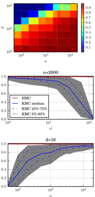
Hamiltonian Monte Carlo (HMC) [86] is an MCMC algorithm that im-proves efficiency by exploiting gradient information. It simulates particle movement along the contour lines of a dynamical system constructed from the target density. Projections of these trajectories cover wide parts of the target’s support, and the probability of accepting a move along a trajectory is often close to one. Remarkably, this property is very robust to growing dimensionality, and HMC here often is superior to random walk methods, which need to decrease their step size at a much faster rate [86, Section 4.4]. Unfortunately, as discussed earlier, for a large class of problems gra-dient information is not available. In those cases, HMC cannot be applied, leaving random walk methods as the only mature alternative.

Contribution.We extend the above idea of using kernel methods to learn local covariance structure for efficient proposal distributions. Rather than

locally smoothing the target density, however, we estimate its gradients

globally. This leads to a kernel-based gradient-free adaptive MCMC algo-rithm, (KMC), that starts as a random walk and then smoothly transitions into HMC-like behaviour. In experiments, KMC outperforms random walk based sampling methods, including the earlier kernel adaptive Metropolis-Hastings. As the latter, KMC is does not require access to target gradients, but estimates those from the sample path only.

Related work.Gaussian Processes (GP) were used by Rasmussen [90] as a surrogate of the target density in order to speed up HMC, however, this requires access to the target in closed form, to provide training points for the GP. More recently, neural networks were used for the same purpose [136]. There have been efforts to mimic HMC’s behaviour using stochastic gradients from mini-batches in ‘Big Data’ [31], or stochastic finite differ-ences in approximate Bayesian computation [82, discussed in Section 4.4.4]. Stochastic gradient based HMC methods, however, often suffer from low acceptance rates or additional bias that is hard to quantify [20].

Score estimation for kernel exponential families

The gradient estimator in KMC is based on a recently proposed proce-dure to fit ainfinite dimensionalexponential family models to sample points drawn i.i.d. from a probability density [117]. While finite dimensional ex-ponential families are a keystone of parametric statistics [25, 126], it is difficult to construct a practical, consistent maximum likelihood solution for infinite dimensional natural parameters [15, 47, 57]. Sriperumbudur et al. [117] proposed to employ a score matching procedure [63], which minimizes the Fisher distance: the expected squared distance between the model score (i.e. the derivative of the log model density) and the score of the (unknown) true density. The Fisher distance can be recast to yield a quadratic loss using integration by parts. Unlike the maximum likelihood case, a solution can be formulated to obtain a well-posed and straightfor-ward solution, which is a linear system defined in terms of the first and

second derivatives of the RKHS kernels at the sample points.

We require our adaptive MCMC algorithms to be computationally ef-ficient yet expressive, as they deal with high-dimensional MCMC chains of growing length. For a practical implementation, it is necessary to ap-proximate the full solution from [117], which has quadratic memory costs and cubic computational costs in both number of samples and dimension. Despite being useful for the developed MCMC proposals, efficiently esti-mating the natural parameter of such an infinite dimensional exponential family model is a challenging problem on its own.

Contribution.We develop two novel approximations for the kernel expo-nential family model. The first approximation, score matching lite, is based on computing the solution in terms of a lower dimensional, yet growing, and simpler subspace in the RKHS. The second approximation uses a fi-nite dimensional feature space (score matching finite), combined with ran-dom Fourier features [89]. These approximations greatly reduce computa-tional costs, and can be used on their own or within the gradient-free HMC framework described above.

Related work.This setting of score estimation is closely related to that of

energy-based learning [72]. For example, Alain and Bengio [2] proposed a deep learning-based approach to directly learn a score function from sam-ples: de-noising auto-encoders are networks trained to recover the original inputs from noise-corrupted versions. We come back to this approach in Chapter 6 where we describe the method in Chapter 6 and compare our methods experimentally in Section 6.3.

Despite the Hamiltonian Monte Carlo context in Chapter 4, the score function is used for constructing control functionals for Monte Carlo inte-gration [88], where learned score functions could be used where closed-form expressions do not exist.

The form of score matching lite is similar to an estimator by Hyvärinen [64], which we will comment on in Section 4.2.1.

Kernel sequential Monte Carlo

In contrast to MCMC, sequential Monte Carlo (SMC) methods are based on iterative importance sampling, and have traditionally been applied to inference in filtering problems with a sequence of time-varying target dis-tributions [39]. We focus on static SMC methods for Bayesian inference on a fixed target distribution [29, 32, 43, 105]. Static SMC frames infer-ence as a sequential problem by defining an artificial series of incremental targets. This can be done by tempering the target density [105], by includ-ing data points sequentially [32], or by targetinclud-ing the full density at every iteration. The latter is a special case known as population Monte Carlo (PMC) [28]. SMC offers three striking advantages over MCMC: adaptive proposal mechanisms do not compromise convergence, normalising con-stants (e.g. model evidence) can be estimated in a straightforward manner, and the particle system can represent multi-modality (where MCMC often gets ‘stuck’ in a single mode).

Contribution.We develop a framework for kernel sequential Monte Carlo,

(KSMC). Similarly to the presented work in adaptive MCMC proposals, KSMC represents the (weighted) particle system of SMC algorithms in an RKHS. The learned structure of the surrogate model is used to construct proposal distributions that are used within SMC. We exemplify this frame-work with two existing SMC algorithms, again based on covariance and gradients. KSMC enjoys the benefits that SMC has over MCMC, yet the use of kernel surrogates leads to faster convergence for non-linear targets as compared to plain SMC. As before, KSMC does not require target gra-dient information and therefore is particularly useful in combination with importance sampling frameworks that are based around intractable targets [33, 125].

Related work.Our algorithms are kernel-based generalisations of adap-tive SMC [43] and gradient importance sampling [102]. We briefly discuss these algorithms in Section 5.1.2. The local adaptive importance sampling

approach by Givens and Raftery [51] adapts to local covariance structure of the target, by computing pairwise distances and then only using a small number of close points to estimate local covariance.

1.3.2

Efficient and principled score estimation

Coming back to approximating the kernel exponential family described in Section 1.3.1, we now focus on the question of developing efficient estima-tors that are theoretically well justified. Indeed, one of the desirable prop-erties of the original estimator by Sriperumbudur et al. [117] is established theory on consistency, with error guarantees depending on the smoothness of the data-generating density.

Contribution.While the approximations in Chapter 4 greatly improve the runtime, no convergence guarantees are known, nor any means of deter-mining how quickly to increase the complexity of these solutions with increasing sample size n. We here develop a learning scheme using the framework of Nyström approximation [112, 130]: representing the solution of the score matching optimisation problem in a sub-space of the original solution. We prove guarantees on the convergence of this algorithm for an increasing number m of Nyström basis points. Depending on the prob-lem difficulty, convergence is attained in the regime m∼n1/3 to m∼n1/2, thus yielding cost savings at the same level of guaranteed generalisation error. The overall Fisher distance between our solution and the true den-sity decreases as m,n_→∞ with rates that match those of the full solution in [117, Theorem 6]. An experimental evaluation confirms the performance benefits in practice.

Related work.Guarantees on the performance of Nyström methods have been the topic of considerable study. Earlier approaches have worked by first bounding the error in a Nyström approximation of the kernel matrix on the sample [41], and then separately evaluating the impact of regression with an approximate kernel matrix [37]. This approach, however, results in suboptimal rates; better rates can be obtained by considering the whole

problem at once [42], including its direct impact on generalisation error [99]. Approaches like those of [42, 134], which bound the difference in training error of Nyström-type approximations to kernel ridge regression, are insufficient for our purposes: we need to ensure that the estimated un-normalised log-density converges to the truth everywhere, so that the full distribution matches, not just its values at the training points. In doing so, our work is heavily indebted to Caponnetto and De Vito [27], as are Rudi et al. [99] and Sriperumbudur et al. [117].

1.3.3

Goodness-of-fit testing

Further downstream the pipeline of sampling algorithms, the effectiveness of any Monte Carlo algorithm strongly depends on the quality of the used random samples. This is in particular true for approximate sampling meth-ods, which use modifications to Markov transition kernels that improve mixing speed at the cost of introducing asymptotic bias [12, 68, 128]. The resulting bias-variance trade-off can usually be tuned with parameters of the sampling algorithms. It is therefore important to test whether for a par-ticular parameter setting and run-time, the samples are of the desired qual-ity. This question cannot be answered with classical MCMC convergence statistics, such as the widely used potential scale reduction factor (R-factor) [49] or the effective sample size, since these assume that the Markov chain reaches the true equilibrium distribution i.e. absence of asymptotic bias.

We address this question using statistical tests of goodness-of-fit, which are a fundamental tool in statistical analysis, dating back to the test of Kolmogorov and Smirnov [67, 109]. Given a set of samples from a dis-tribution q, our interest is in whether q matches some reference or target distribution p, which we assume to be only known up to the normalisation constant.

Recently, in the multivariate setting, Gorham and Mackey [52] pro-posed an elegant measure of sample quality with respect to a target. This measure is a maximum discrepancy between empirical sample expectations

and target expectations over a large class of test functions, constructed so as to have zero expectation over the target distribution by use of a Stein op-erator. This operator depends only on the derivative of the logq: thus, the approach can be applied very generally, as it does not require closed-form integrals over the target distribution (or numerical approximations of such integrals). This property is particularly useful in assessing MCMC, since these integrals are certainly not known to the practitioner.

An important application of a goodness-of-fit measure is in statistical testing, where it is desired to determine whether the empirical discrepancy measure is large enough to reject the null hypothesis (that the sample arises from the target distribution) with a certain p-value. One approach is to establish the asymptotic behaviour of the test statistic, and to set a test threshold at a large quantile of the asymptotic distribution.

Contribution.We define a statistical test of goodness-of-fit, based on a Stein discrepancy computed in an RKHS. To construct our test statistic, we use a function class defined by applying the Stein operator to a chosen space of RKHS functions, as proposed by Oates et al. [88].1 Our measure of goodness of fit is the largest discrepancy over this space of functions between empirical sample expectations and target expectations (the latter being zero, due to the effect of the Stein operator). The approach is a natu-ral extension to goodness-of-fit testing of the earlier kernel statistical tests [54, 55], which are based on themaximum mean discrepancy, c.f. Section 2.1. As with these earlier tests, our statistic is a simple V-statistic, and can be computed in closed form and in quadratic time in the number of samples. Moreover, it is an unbiased estimate of the corresponding population dis-crepancy. Only the gradient of the log target density is needed; we do not require integrals with respect to the target density – including the nor-malisation constant, which makes the test well suited for MCMC samples. We make use of the extensive literature on asymptotics of V-statistics to

1_{Oates et al. addressed the problem of variance reduction in Monte Carlo integration,}

formulate a hypothesis test [74, 106] and provide statistical tests for both uncorrelated and correlated samples, where the latter is essential if the test is used in assessing the quality of output of an MCMC procedure.

Related work.Several alternative approaches exist in the statistics litera-ture to goodness-of-fit testing. A first strategy is to partition the space, and to conduct the test on a histogram estimate of the distribution [14, 17, 58, 59]. Such space partitioning approaches can have attractive theoreti-cal properties (e.g. distribution-free test thresholds) and work well in low dimensions, however they are much less powerful than alternatives once the dimensionality increases [56]. A second popular approach has been to use the smoothed L2distance between the empirical characteristic function of the sample, and the characteristic function of the target density. This dates back to the test of Gaussianity of Baringhaus and Henze [13, Equa-tion 2.1], who used an exponentiated quadratic smoothing funcEqua-tion. For this choice of smoothing function, their statistic is identical to the maxi-mum mean discrepancy, c.f. Section 2.1, with the exponentiated quadratic kernel, which can be shown using the Bochner representation of the kernel [115, Corollary 4]. It is essential in this case that the target distribution be Gaussian, since the convolution with the kernel (or in the Fourier domain, the smoothing function) must be available in closed form. An L2 distance

between Parzen window estimates can also be used [24], giving the same expression again, although the optimal choice of bandwidth for consis-tent Parzen window estimates may not be a good choice for testing [3]. A different smoothing scheme in the frequency domain results in an energy distance statistic (this likewise being an MMD with a particular choice of kernel; see Sejdinovic et al. [103]), which can be used in a test of normality [124]. The key point is that the required integrals are again computable in closed form for the Gaussian, although the reasoning may be extended to certain other families of interest, e.g. [91]. The requirement of computing closed-form integrals with respect to the test distribution severely restricts

this testing strategy. Finally, a problem related to goodness-of-fit testing is that of model criticism [79]. In this setting, samples generated from a fitted model are compared via the maximum mean discrepancy, c.f. Section 2.1, with samples used to train the model, such that a small MMD indicates a good fit. There are two limitation to the method: first, it requires samples from the model (which might not be easy if this requires a complex MCMC sampler); second, the choice of number of samples from the model is not obvious, since too few samples cause a loss in test power, and too many are computationally wasteful. Neither issue arises in our test, as we do not require model samples.

An identical test (for uncorrelated samples) was independently devel-oped at the same time by Liu et al. [77].

Thesis structure

We begin by introducing a minimal amount of necessary concepts and no-tations in Chapter 2. This includes basics of reproducing kernel Hilbert spaces in Section 2.1, score matching in Section 2.2, and Markov chain Monte Carlo in Section 2.3.

Part I – Adaptive Monte Carlo proposals

We introduce three contributions for using kernel methods in adaptive MCMC transition kernels. Chapter 3 is based on modelling covariance in an RKHS for proposals that locally align with the target density. Chap-ter 4 is based on modelling the score to mimic Hamiltonian dynamics and develops fast approximations to existing kernel-based score learning meth-ods. Chapter 5 applies these concepts to the context of sequential Monte Carlo.

Part II – Efficient and principled score estimation

Chapter 6 provides yet another fast approximate kernel-based score learn-ing method, which is a generalisation of those described in Chapter 4. The method’s theoretical foundations are explored in a longer technical proof

in Chapter 7.

Part III – Goodness-of-fit testing

Chapter 8 introduces a novel kernel goodness-of-fit test for measuring the quality of MCMC samples, and for assessing convergence of the score esti-mation models from Chapter 4.

Part IV – Conclusions

We finally conclude, and discuss potential future work and recent develop-ments related to this work.

Background

We now introduce concepts and notation that is used throughout the rest of the thesis.

2.1

Reproducing kernel Hilbert spaces

Reproducing kernel and feature map

According to the Moore-Aronszajn theorem [19, page 19], for every sym-metric, positive definite function (kernel)

k:_{X × X →}R

there is an associated RKHS H of real-valued functions on X with repro-ducing kernelk, that is

hk(·,x),f)iH = f(x) ∀f ∈ H. (2.1)

The map ϕ:X → H, with

ϕ:x7→k(·,x), (2.2)

is called the(canonical) feature mapofk. The reproducing property (2.1) also holds for for kernel derivatives, as long as k is differentiable [119, Lemma

4.34], ∂ ∂xi k(_·,x),f H = ∂ ∂xi f(x) _∀f _{∈ H}, (2.3)

which can be generalised to higher-order derivatives as well.

Mean embedding

This feature map or embedding of a single point can be extended to that of a probability measure PonX: its kernel embedding is an elementµP∈ H, given by

µP= Z

k(·,x)dP(x)

[19, 46, 111]. If a measurable kernel k is bounded, it is straightforward to show using the Riesz representation theorem that the mean embeddingµP exists for all probability measures on X. For many interesting bounded kernels k, including the Gaussian, Laplace and inverse multi-quadratics, the kernel embedding P7→ µP is injective. Such kernels are said to be characteristic[114, 115], since each distribution is uniquely characterized by its embedding. The kernel embeddingµPis the representer of expectations of smooth functions w.r.t. P, i.e.

hf,µPi_H= Z

f(x)dP(x) ∀f ∈ H.

Given samples X=_{Xi}ni=1∼P, the embedding of the empirical measure

isµX= _n1∑ni=1k(·,Xi), i.e. the sample mean in feature space.

Covariance operator

Denote by CP : H → H the covariance operator for a probability measure P [10, 46], which satisfies

CP= Z

where fora,b,c∈ Hthe tensor product is defined as

(a_⊗b)c=_hb,c_iHa. (2.5) The covariance operator has the property that

hf,CPgi_H=EP(f g)−EPfEPg ∀f,g∈ H.

Analogous to the mean in feature space, we can think of the covariance operator as the generalisation of the covariance matrix in feature space.

Maximum mean discrepancy

The MMD [22, 53, 54] is a measure of distance for two random variables

x∼P,y∼Q, here defined in a unit ball in an RKHSH,

sup

kfkH=1

(EP f(x)−EQ f(y)) =kµP−µQkH,

where the right hand side is an interpretation as the mean difference of the random variables embedded in the RKHS, c.f. mean embedding. The equality can be showed using simple RKHS arguments [53, Lemma 4]. The MMD can be estimated from samples {Xi}ni=1,{Yj}mj=1 in quadratic time,

for example as 1 n(n−1) n

∑

∑

∑

∑

∑

∑

Measuring convergence of mixed third order moments.Throughout the experimental section of the paper, we will use the empirical MMD in the RKHS of the third order polynomial kernel

The corresponding (finite dimensional) RKHS captures all mixed moments up to order three, i.e. an empirical estimate quantifies how close two sets of samples are in terms of such moments in a single quantity. We will compare a reference set of samples from a long MCMC chain with outputs of sampling algorithms.

Kernel parametrization of exponential families

We now describe the kernelorinfinite dimensional exponential family[26, 47]. This is a generalisation of the standard exponential family model [126]. The model class is defined as a set of density functions

P =pf(x):=exp(f(x)−A(f))q0(x)| f ∈ F , (2.6) where_{F ⊆ H}is the set of functions in the RKHS _Hfor which the normal-izer

A(f) =logZ(pf) Z(pf) = Z

exp(f(x))q0(x)dx (2.7)

is finite, and q0 is a base measure with appropriately vanishing tails. That this is a member of the exponential family becomes apparent when we re-call the reproducing property (2.1): the feature mapx7→k(x,·)in (2.2) is the sufficient statistic, and f is the natural parameter whose evaluation by the reproducing property (2.1) is the inner product with the sufficient statistic,

f(x) =_hk(x,_·),f_iH. An overview of various finite dimensional members of the exponential family (such as Gamma, Poisson, Binomial, etc.) and their corresponding kernel functions may be found in [117, Example 1]. The model (2.6) defines broad class of densities: when universal kernels are used, the family is dense in the space of continuous densities on compact domains, with respect to e.g. total variation distance and Kulback-Leibler divergence [117, Section 3].

Unfortunately, fitting (2.6) by maximum likelihood becomes impracti-cal in high dimensions, and is ill-posed in infinite dimensions, due to the

intractability of A(f) [15, 57], [47, Section 1.3.1]. It is, however, possible to consistently fit anun-normalisedversion of (2.6) by directly minimising the expected gradient mismatch between the model (2.6) and the data gener-ating density. This is achieved by generalising a score matching approach [63, 117] to RKHS parameter spaces. The technique avoids the problem of dealing with the intractable A(f) in (2.7), and reduces the problem to solving a linear system. We describe the estimator below.

2.2

Score matching & un-normalised density

es-timation

Suppose we are given a set of points X =_{Xb}b∈[n] ⊂Rd sampled i.i.d.

from an unknown distribution with density p0. Our setting is that of un-normalised density estimation, where we wish to fit a model p such that

p(x)/Z(p) ≈p0(x) in some divergence measure, and we do not concern ourselves with the normalization factor in (2.7).

Hyvärinen [63] proposed an elegant approach to fit an un-normalised density p0 with a model p, by minimizing the Fisher divergence, the ex-pected squared distance betweenscore functions1 _∇xlogp(x):

J(p0kp) = 1 2 Z p0(x)k∇xlogp(x)− ∇xlogp0(x)k2₂dx (2.8) = Z p0(x) d

∑

where we use∂if(x) to denote _∂∂_xif(x). The equality in (2.9) assumes some mild regularity conditions and contains a constant depending only on p0. Crucially, (2.9) is independent of the normaliser (2.7) and, other than the constant, depends onp0only through an expectation, so it can be estimated by a simple Monte Carlo average.

1_{Here we use the termscorein the sense of Hyvärinen [63], i.e. the gradient of the log}

Kernel exponential families

For the kernel exponential family model (2.6), Sriperumbudur et al. [117, Theorem 3] showed that the score matching loss (2.9) takes a quadratic form (see also Lemma 1 in Chapter 7),

J(p0||pf) = 1 2hf − f0,C(f − f0)iH, where C:_{H → H}, C:= Z p0 d

∑

can be thought of as a ‘covariance between derivatives’ operator similar to the covariance operator (2.4), and f0_{∈ H} is the RKHS function that corre-sponds to the true2 density p0. The expression can be further simplified to J(p0kpf) = 1 2hf,C fiH+hf,ξiH+J(p0kq0), where H 3ξ:= Z p0 d

∑

and where J(p0kq0) is the Fisher divergence between the base measure q0

and the true density (independent of f).

We will mostly use q0 =const throughout this work, which results, intuitively speaking, in_hξ,fi_H=R p0∑di=1∂2i f(x)dx quantifying curvature of f.

Estimation in kernel exponential families

We briefly discuss the score matching approach that Sriperumbudur et al. [117] propose to fit the kernel exponential family model (2.6), i.e. to find an

2_{Note that this assumes the ‘well specified’ case, i.e. there exists an f}

0∈ Hsuch that

f such that pf approximates p0. Their empirical estimator of (2.9) is ˆ J(f) = Jˆ(p0kpf)−const = 1 n n

∑

∑

where the constant depends on p0 and q0 but not on f. Minimizing a regularised version of (2.10) gives

fλ,n =argmin f∈H ˆ J(f) +1 2λkfk 2 H=− ˆ ξ λ + n

∑

∑

∑

∑

combination of ∂ik(Xa,x) and ∂2_ik(Xa,x) for each sample Xa. The weights

β of this linear combination are obtained by solving the nd-dimensional linear system

(G+nλI)β=h/λ, (2.13)

where G_∈Rnd×nd is the matrix collecting partial derivatives of the kernel at the training points,

G_(a,i),(b,j) =∂i∂j+dk(Xa,Xb), and h∈Rnd _{evaluates derivatives of ˆ}

ξ,

Solving (2.13) takes O(n3d3) time and O(n2d2) memory, which quickly becomes infeasible as ngrows, especially for large d.

2.3

Markov chain Monte Carlo

Denote an un-normalised target density on X by π. We are interested in constructing a Markov chain X1 → X2 → · · · → Xt → . . . such that limt→∞Xt∼π. By running the Markov chain for a long timeT, we can con-sistently approximate any expectation w.r.t.π using sample averages using (1.1), [93]. Markov chains are constructed using the Metropolis-Hastings (MH)algorithm, which at the current state xt draws a point from aproposal distribution X∗_∼Q(_·|Xt), and setsXt+1←X∗ with probability

min 1,π(X ∗_)Q(X t|X∗) π(Xt)Q(X∗|Xt) , (2.14) and Xt+1←Xt otherwise.

Exact-approximate inference

Replacing π(x) in (2.14) with an estimator ˆπ(x) that is unbiased, i.e. Eπˆ(x) = π(x) where the expectation is over the estimation random-ness, results in pseudo-marginal MCMC. It is straight-forward to show that the resulting Markov chain retains the same, asymptotically exact, limiting distribution [5, 16].

Random walk (adaptive) Metropolis

One of the simplest (continuous) proposal distributions is a Gaussian, which results in the random walk Metropolisalgorithm. At position Xt, the proposal is sampled from

Qt(·|Xt) =N(· |Xt,νΣ), (2.15) for some user-specified covarianceΣ and (positive)step-sizeν.

Σ prior to running the algorithm is challenging, as the structure of the target is yet unknown. One idea is to learn the global covariance structure on the fly. LetΣt=Σt(X0,X1, . . . ,Xt−1)denote a covariance matrix estimate

obtained from the Markov chain history {Xi}it−=10. The adaptive Metropolis

algorithm [6, 60, 61] replacesΣwith Σt in (2.15),

Qt(·|Xt) =N(· |Xt,νtΣt). (2.16) Adaptive Metropolis therefore considers global covariance structure of the target when proposing moves, which often leads to improved convergence speed.

While adaptive Metropolis was shown to converge to the same correct asymptotic distribution as random walk metropolis under certain condi-tions, this is not necessarily true in general [6, Section 2]. Therefore, care has to been taken when adaptive proposal mechanisms are used.

Step-size adaptation

One choice for the scaling factor νin the Gaussian proposal (2.15) is to use a fixed factor ν=2.38/√d, which was shown to be optimal on Gaussian targets in an asymptotic sense [48]. This result does not generally hold for adaptive Metropolis in (2.16) or for non-Gaussian targets, but it can nevertheless be used as a heuristic. Alternatively, the scale ν can also be replaced with νt, which can be adapted at each step, as in [6, Algorithm 4], to obtain an ‘asymptotically optimal’ the acceptance rate α∗≈0.234 from Gelman et al. [48] and Rosenthal [97]. A simple rule to tune the step-size such that the current acceptance rate αt reaches a desired value α∗ is the stochastic approximation recursion by Robbins and Monro [92], heavily used by the work of Andrieu and Thoms [6],

logνt+1=logνt+λt+1(αt −α∗), (2.17) whereλt is a ‘learning-rate’ parameter.

Adaptive Monte Carlo proposals

Kernel adaptive

Metropolis-Hastings

This chapter is based on collaborative work, D. Sejdinovic, H. Strathmann, M. Lomeli, C. Andrieu, and A. Gretton. “Kernel Adaptive Metropolis-Hastings”. In: International Conference for Machine Learning. 2012.

A kernel adaptive Metropolis-Hastings algorithm is introduced, for the purpose of sampling from a target distribution with strongly non-linear support. The algorithm embeds the trajectory of the Markov chain into a reproducing kernel Hilbert space, such that the feature space covariance of the samples informs the choice of proposal. The procedure is computa-tionally efficient and straightforward to implement, since the RKHS moves can be integrated out analytically: our proposal distribution in the orig-inal space is a normal distribution whose mean and covariance depend on where the current sample lies in the support of the target distribution, and adapts to its local covariance structure. Furthermore, the procedure requires neither gradients nor any other higher order information about the target, making it particularly attractive for contexts such as pseudo-marginal MCMC. Kernel Adaptive Metropolis-Hastings outperforms com-peting fixed and adaptive samplers on multivariate, highly non-linear tar-get distributions, arising in both real-world and synthetic examples.

Chapter outline

Based on the notion of covariance operators in RKHS, c.f. Section 2.1, we describe a sampling strategy for Gaussian measures in the RKHS in Sec-tion 3.1, and introduce a cost funcSec-tion for constructing proposal distribu-tions. In Section 3.2, we outline our main algorithm, termed kernel adap-tive Metropolis-Hastings (MCMC Kameleon). We provide experimental comparisons with other fixed and adaptive samplers in Section 3.3, where we show superior performance in the context of pseudo-marginal MCMC for Bayesian classification, and on synthetic target distributions with highly non-linear shape.

3.1

Sampling in RKHS

Our approach is based on the idea that the non-linear support of a target density may be learned using kernel principal component analysis (ker-nel PCA) [8, 110], which is standard linear PCA [21, Chapter 12] on the empirical version of the covariance operator (2.4) in an RKHS,

CX= 1 n n

∑

computed on a sample{Xi}_in₌₁. The empirical covariance operator behaves as expected from its finite dimensional covariance matrix counterpart: ap-plying the tensor product in definition (2.5) gives

hf,CXgi_H = 1 n n

∑

∑

∑

By analogy with algorithms which use linear PCA directions to in-form MH proposals [6, Algorithm 8], non-linear PCA directions could be encoded in the proposal construction, as we described in Sejdinovic et al. [104, Appendix]. Alternatively, the approach we pursue here is to focus on a Gaussian measure in the RKHS determined by the empirical

covari-ance operatorCX. This generalises the proposal (2.16) by Haario et al. [60], which considers the Gaussian measure induced by the empirical covariance matrix on the original space.

We next describe the proposal distribution at iterationt of the MCMC chain. We assume that a subset of the chain history, denoted X=_{Xi}ni=1, n_≤t₋1, is available. Our proposal is constructed by first directly sam-pling from the density induced by the empirical covariance operator in the RKHS, and then performing a gradient descent in order to find a corre-sponding location in input space. The gradient step’s cost function solely depends on the embedded Markov chain history into the RKHS. We finally add exploration noise.

As we will see later, it is possible to simplify the procedure by integrat-ing out the samplintegrat-ing in the RKHS, the gradient step, and the exploration noise altogether, leading to a closed-form proposal.

3.1.1

Gaussian measure of the covariance operator

We work with the Gaussian measure on the RKHS H with mean k(·,Xt) and covariance ν2CX, where X = {Xi}ni=1 is the subset of the chain

his-tory1. While there is no analogue of a Lebesgue measure in an infinite dimensional RKHS, it is instructive (albeit with some abuse of notation) to denote this measure in the ‘density form’

N(f _| k(_·,Xt),ν2CX)∝exp − 1 2ν2 D f ₋k(_·,Xt),C_X−1(f −k(·,Xt)) E H . (3.1) AsCX is a rank operator, this measure is supported only on a finite-dimensional affine spacek(_·,Xt) +HX, whereHX=span{k(·,Xi)}in=1is the

subspace spanned by the canonical features of X. Conveniently, samples

1_{We assume w.l.o.g. thatXcontains the firstnof alltdata, i.e.{X}

from this measure take the form f =k(_·,Xt) + n

∑

is isotropic. The sample mean is

E[f] =E " k(_·,Xt) + n

∑

and the sample covariance is

E[(f −k(·,Xt))⊗(f −k(·,Xt))] =E " n

∑

∑

∑

∑

∑

which exactly coincides with (3.1).

3.1.2

Obtaining proposals through gradient descent

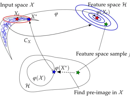
The RKHS sample f =k(·,Xt) +∑ni=1βi[k(·,Xi)−µX] represents the non-linear covariance structure of the Markov chain history, and therefore would be a useful proposal. Unfortunately, this sample does not in gen-eral have a corresponding pre-image in the original domain X =Rd_{, i.e.} there is no point X_∗ ∈ X such that f =k(·,X_∗). If there were such a point, then we could use it as a proposal in the original domain, as illustrated

ϕ(X) H

ϕ

CX

Feature space sample f X∗ Xt ϕ(X∗) ϕ(Xt) Find pre-image inX Feature spaceH Input spaceX

Figure 3.1: Illustration of embedding the Markov chain history into RKHS, sam-pling from the corresponding empirical Gaussian measure, and taking a gradient step to find the sample’s pre-image.

in Figure 3.1. Therefore, we are ideally looking for a point X∗∈ X whose canonical feature map k(_·,X∗) is close to f. A natural way to quantify ‘closeness’ here is the RKHS norm, which allows to translate the problem of finding the pre-image into an optimisation problem,

argmin x∈X k k(·,x)− fk2_H =argmin x∈X ( k(x,x)−2k(x,Xt)−2 n

∑

where we implicitly defined the kernel induced cost functiong(x). In gen-eral, this is a non-convex minimisation problem, and may be difficult to solve [11]. Rather than solving it for every new vector of coefficients β, which would lead to an excessive computational burden for every pro-posal made, we instead take a single descent step along the gradient of g

in (3.3). The proposed new point is

X∗ =Xt−η∇xg(x)|x=Xt +ξ,

whereηis a gradient step-size parameter andξ∼ N(0,γ2I)is an additional isotropic ‘exploration’ term added afterthe gradient step. This exploration noise avoids the proposal to collapse in unexplored regions, and thereby ensures the proposal to fall back to an isotropic random walk2.

It is useful to split the scaled gradient at Xt into two terms as

η∇xg(x)|x=Xt =η(aXt −MX,XtHβ), whereaXt =∇xk(x,x)|x=Xt−2∇xk(x,Xt)|x=Xt,

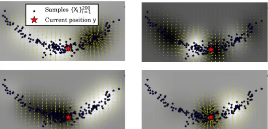
MX,Xt =2[∇xk(x,X1)|x=Xt, . . . ,∇xk(x,Xn)|x=Xt] (3.4) is a d_×n matrix, and H = I_{− n}11n×n is the n×n centering matrix. Fig-ure 3.2 shows g(x) and its gradients for several samples of β-coefficients, in the case where the underlyingX-samples are from the two-dimensional nonlinear Banana target distribution of Haario et al. [60] that we will use in Section 3.3.2. It can be seen thatgmay have multiple local minima, and that it varies most along the high-density regions of the Banana distribution.

3.2

MCMC Kameleon algorithm

We now have a recipe to construct a proposal that is able to adapt to the local covariance structure for the current chain state Xt. While we will simplify this proposal by integrating out the moves in the RKHS, it is in-structive to think of the proposal generating process as:

1. Sample β∼ N(0,ν2I), nreal-valued RKHS coefficients.

2_{We will see in Chapter 4 that this property translates into the fact that our algorithm}

Samples{Xi}200i = 1

Current positiony

Figure 3.2: Heatmaps (white denotes large) and gradients ofg(x)for four samples of βand fixed{Xi}n_i=1 (blue), at the current positiony=Xt (red).

This represents an RKHS sample

f =k(·,Xt) + n

∑

i=1

βi[k(·,Xi)−µX] which induces the cost function g(x).

2. Move along the gradient of g and add noise ξ∼ N(0,γ2I), i.e. X∗=

Xt−η∇xg(x)|x=Xt, d-dimensional in the original space This gives a proposal

X∗|Xt,β,ξ ∼ N(X∗|Xt−ηaXt+ηMX,XtHβ,γ

2_{I). (3.5)}

3.2.1

Closed form proposal

As the the explicit sampling of f in the RKHS, the (deterministic) gradient step, and the addition of exploration noise only involve Gaussian distri-butions, the procedure can be integrated out analytically. This leads to a

closed formGaussian proposal whose covariance matrix locally aligns to the target covariance structure observed through the Markov chain history.

The first step in the derivation of the explicit proposal density is to show that as long ask is a differentiable positive definite kernel, the term

aXt vanishes. Derivations of the following result are given in [104, Ap-pendix].

Proposition 1. Let k be a differentiable positive definite kernel. Then aXt =∇xk(x,x)|x=Xt −2∇xk(x,Xt)|x=Xt =0.

Since aXt =0, the gradient step-sizeη in (3.5) always appears together with β, we mergeη and the scaleνof theβ-coefficients in (3.2) into a single scale parameter, and set η =1 henceforth. Furthermore, since both β and

X∗_|Xt,β,ξ admit multivariate Gaussian densities, the proposal density can be computed via integrating over βand ξ,

QX(X∗|Xt) = Z

p(X∗_|Xt,β,ξ)p(β)p(ξ)dβdξ,

where p(X∗|Xt,β,ξ) is the density of the explicit proposal in (3.5): an isotropic Gaussian whose mean is shifted according to the kernel gradi-ents from (3.4). We arrive at the following closed form expression for the proposal distribution, a simple multivariate Gaussian density.

Proposition 2. QX(X∗|Xt) =N(X∗|Xt,γ2I+ν2MX,XtHM>X,Xt).

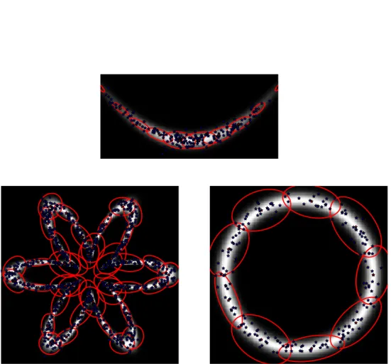
Figure 3.3 depicts contours of the proposal distribution QX(·|Xt) at various states Xt for a fixed subsample X from various targets (target de-tails in Section 3.3.2).

With the simplified proposal distribution in Proposition 2, we proceed with the standard Metropolis-Hastings accept/reject scheme (2.14), where the proposed sampleX∗ is accepted with probability

α(Xt,X∗):=min 1,π(X ∗_)Q X(Xt|X∗) π(Xt)QX(X∗|Xt) , (3.6)

Figure 3.3: 95% contours (red) of proposal distributions evaluated at a number of points, for the first two dimensions of the banana target of Haario et al. [60], and ring and flower. Underneath is the density heatmap, and the samples (blue) used to construct the proposals.

could be replaced by their unbiased estimates without impacting the in-variant distribution [5].

MCMC Kameleon

Input: un-normalised target π, subsample size n, scaling parameters ν,γ, adaptation probabilities _{at}∞_t=0, kernelk,

• At iterationt+1,

1. With probabilityat, update a random subsampleX={Xi}_imin₌₁(n,t) of the chain history_{Xi}ti=−10,

2. Sample proposed point x∗ from QX(·|Xt) = N(· | Xt,γ2I + ν2MX,XtHMX>,Xt), where MX,xtis given in (3.4) andH=I−

1 n1n×n is the centering matrix,

3. Accept or reject with the Metropolis-Hastings acceptance proba-bility in (3.6),

Xt+1 ← (

X∗, with probability α(Xt,X∗), Xt, with probability 1−α(Xt,X∗).

3.2.2

Properties of the Algorithm

Update schedule and convergence.

MCMC Kameleon requires a subsampleX=_{Xi}n_i=1at each iteration of the algorithm, and the proposal distribution QX(·|Xt) is updated each time a new subsample X is obtained. It is well known that a chain which keeps adapting the proposal distribution need not converge to the correct tar-get [6]. To guarantee convergence, we introduce adaptation probabilities {at}∞_t=0, such that at →0 and ∑∞_t=1at =∞, and at iteration t we update the subsample X with probability at. As adaptations occur with decreas-ing probability, Roberts and Rosenthal [94] implies that the resultdecreas-ing al-gorithm is ergodic and converges to the correct target. Another straight-forward way to guarantee convergence is to fix the set X=_{Xi}in=1 after

a ‘burn-in’ phase, i.e. to stop adapting altogether [94, Proposition 2]. In this case, a ‘burn-in’ phase is used to get a rough sketch of the shape of

the distribution: the initial samples need not come from a converged or even valid MCMC chain, and it suffices to have a scheme with good ex-ploratory properties, e.g. Welling and Teh [129]. In MCMC Kameleon, the term γ allows exploration in the initial iterations of the chain (while the subsample X is still not informative about the structure of the target) and provides regularisation of the proposal covariance in cases where it might become ill-conditioned. Intuitively, a good approach to setting γ is to slowly decrease it with each adaptation, such that the learned covari-ance progressively dominates the proposal. We will return to the question of convergence speed in the case of pre-mature stopping of the update in Chapter 4.

Symmetry

In Haario et al. [61], the proposal distribution is asymptotically symmetric due to the vanishing adaptation property. Therefore, the authors compute the standard Metropolis acceptance probability, i.e. the proposal density ratio in the MH acceptance probability in (3.6) is equal to one. In our case, the proposal distribution is a Gaussian with mean at the current state of the chainXt and covarianceγ2I+ν2MX,XtHM>X,Xt, whereMX,Xt depends both on the current state Xt and a random subsampleX={Xi}ni=1 of the chain

history {Xi}ti=−01. This proposal distribution is never symmetric (as

covari-ance of the proposal always depends on the current state of the chain), and therefore we use the Metropolis-Hastings acceptance probability to reflect this.

3.2.3

Examples of covariance structure for standard kernels

The proposal distributions in MCMC Kameleon are dependent on the choice of the kernel k. To gain intuition regarding their covariance struc-ture, we give two examples.

Linear kernel

In the case of a linear kernel k(x,x0) =x>x0, we obtain

MX,Xt =2

h

∇xx>X1|x=Xt, . . . ,∇xx>Xn|x=Xt

i

=2X>, so the proposal is given by

QX(·|Xt) =N(Xt,γ2I+4ν2X>HX).

Thus, the proposal uses the scaled empirical covarianceX>HX, with an ad-ditional isotropic exploration component, and depends onXt only through the mean. MCMC Kameleon therefore is a generalisation of the adaptive Metropolis algorithm [60].

Gaussian kernel

In the case of a Gaussian kernel k(x,x0) = exp

−kx−x0k22 2σ2 , since ∇xk(x,x0) = _σ12k(x,x0)(x0−x), we obtain MX,Xt = 2 σ2[k(Xt,X1)(X1−Xt), . . . ,k(Xt,Xn)(Xn−Xt)].

Consider how this encodes the covariance structure of the target distribu-tion, with the(i,j)-th entry given by

γ2δi=j + 4ν2(n−1) σ4n n

∑

∑

As the first two terms dominate, the previous points Xa which are close to the current state Xt (for which k(Xt,Xa) is large) have larger weights, and thus they have more influence in determining the covariance of the proposal at Xt.

3.3

Experiments

In the experiments, we compare the following samplers:

• (SM) Standard Metropolis with the isotropic proposal Q(·|Xt) =

N(Xt,ν2I)and scaling ν=2.38/√d

• (AM-FS)Adaptive Metropolis with a learned covariance matrix and fixed scalingν=2.38/√d

• (AM-LS)Adaptive Metropolis with a learned covariance matrix and scaling learned to bring the acceptance rate close toα∗=0.234 using (2.17).

• (KAMH-LS)MCMC Kameleon with the scalingνlearned in the same fashion (γ was fixed to 0.2), and which also stops adapting the pro-posal after the burn-in of the chain

In all experiments, we use a random sub-sample X of the Markov chain history of size n=1000, and a Gaussian kernel with bandwidth selected according to the median heuristic3. We consider the following non-linear targets:

• the posterior distribution of Gaussian Process classification hyper-parameters [44] on the UCI glass dataset

• the synthetic banana-shaped distribution of Haario et al. [60] and a flower-shaped distribution concentrated on a circle with a periodic perturbation

3.3.1

Pseudo-marginal MCMC for Bayesian classification

In the first experiment, we illustrate usefulness of the MCMC Kameleon sampler in the context of Bayesian classification with GPs [131]. Variants of this experiment will be used in Chapter 4, Chapter 5, and Chapter 6.

3_{The median heuristic matches the bandwidth of a Gaussian kernel with the median}

Set-up

Consider the joint distribution of latent function responses f _∈ Rn, labels

y∈ {−1, 1}n_{, and hyper-parameters}

θ, given by

p(f,y,θ) = p(θ)p(f|θ)p(y|f),

where f|θ ∼ N(0,Kθ), with Kθ modelling the covariance between latent

function values evaluated atd-dimensional input covariatesxa,xb:

(_Kθ)ab=κ(xa,xb|θ) =exp − 1 2 d

∑

and θi=log`2_i. We restrict our attention to the binary logistic classifier, i.e. the likelihood is given by

p(yi|fi) =

1

1−exp(−yifi),

where yi ∈ {−1, 1}. We pursue a fully Bayesian treatment, and estimate the posterior of the hyper-parameters θ. As observed by Murray and Adams [84], a Gibbs sampler on p(θ,f|y), which samples fromp(f|θ,y)and

p(θ|f,y) in turn, is problematic, as p(θ|f,y) is extremely sharp, drastically limiting the amount that any Markov chain can updateθ|f,y. On the other hand, if we directly consider the marginal posterior p(θ|y)∝ p(y|θ)p(θ) of the hyper-parameters, a much less peaked distribution can be ob-tained. The marginal likelihood p(y_|θ), however, is intractable for the non-Gaussian likelihood p(y|f), so it is not possible to analytically integrate out the latent variables. Pseudo-marginal MCMC methods, c.f. Andrieu and Roberts [5] and Section 2.3, enableasymptotically exactinference on this problem, by replacing p(y_|θ) with an unbiased estimate. Such an estimate

−6 −5 −4 −3 −2 −1 0 θ2 −5 −4 −3 −2 −1 0 θ7

Figure 3.4: Dimensions 2 and 7 of the marginal hyperparameter posterior on the UCI Glass dataset

can for example be obtained via importance sampling,

ˆ p(y_|θ):= 1 nimp nimp

∑

i=1 ∼q(f|θ) are nimp importance samples form a tractable

distributionq(f_|θ)

Filippone and Girolami [44] applied this idea to the presented GP clas-sification framework and obtained state-of-the-art results in terms of accu-racy of predictions and uncertainty quantification. The importance distri-bution q(f|θ) is chosen as the Laplace or as the expectation propagation (EP) approximation of p(f_|y,θ)∝ p(y|f)p(f|θ).

Data

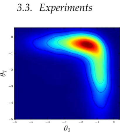
We consider the UCI glass dataset [9], where classification of window against non-window glass is sought. Due to the heterogeneous structure of each of the classes (i.e. non-window glass consists of containers, tableware and headlamps), there is no single consistent set of length-scales determin-ing the decision boundary, so one expects the posterior of the covariance bandwidthsθdto have a complicated (non-linear) shape. This is illustrated by the plot of the posterior projections to the dimensions 2 and 7 (out of 9) in Figure 3.4.

Experimental protocol

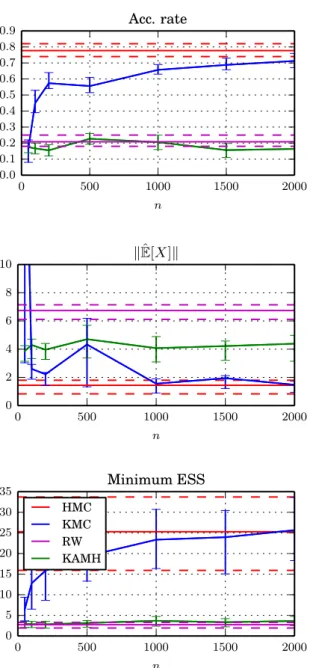
Since the ground truth for the hyper-parameter posterior is not available, we initially run 30 standard Metropolis chains for 500,000 iterations (with a 100,000 burn-in), keep every 1000-th sample in each of the chains, and combine them. The resulting samples are used as a benchmark, to evaluate the performance of shorter single-chain runs of SM, AM-FS, AM-LS and KAMH-LS. We execute each of these algorithms for 100,000 iterations (with a 20,000 burn-in) and keep every 20-th sample.

Results

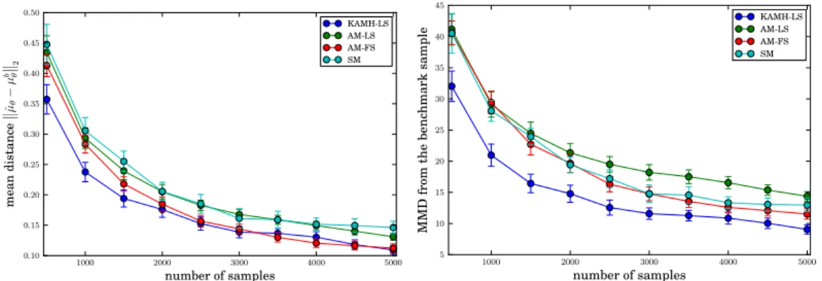
We use two metrics for evaluating the performance, always relative to the large-scale benchmark sample. First, we compute the Euclidean distance of empirical mean of the sampler output ˆµθ and the mean of the benchmark

samplesµb_θ, µˆθ−µ b θ ₂,

as a function of sample size (Figure 3.5, left). Second, in order to quan-tify convergence in higher order moments, we estimate the MMD using a third order polynomial kernel, c.f. Section 2.1, between each sampler out-put and the benchmark sample (Figure 3.5, right). The figures indicate that KAMH-LSapproximates the benchmark sample better than the competing approaches, where the effect is especially pronounced in the high order moments, indicating that KAMH-LS thoroughly explores the distribution support in a relatively small number of samples.

Computational costs

The bulk of the cost for pseudo-marginal MCMC is in importance sam-pling in order to obtain the acceptance ratio. Therefore, the additional cost imposed byKAMH-LS is negligible. Indeed, we observed that there is an increase of only 2-3% in terms of effective computation time in comparison to all other samplers, for the chosen size of the chain history sub-sample (n=1000).

1000 2000 3000 4000 5000 number of samples 0.10 0.15 0.20 0.25 0.30 0.35 0.40 0.45 0.50 m ea n di st an ce ˆ µθ − µ b θ 2 KAMH-LS AM-LS AM-FS SM 1000 2000 3000 4000 5000 number of samples 5 10 15 20 25 30 35 40 45 M M D fr om th e be nc hm ar k sa m pl e KAMH-LSAM-LS AM-FS SM

Figure 3.5: The comparison ofSM,AM-FS,AM-LSandKAMH-LSin terms of the distance between the estimated mean and the mean on the benchmark sample (left) and in terms of the maximum mean discrepancy to the benchmark sample (right). The results are averaged over 30 chains for each sampler. Error bars represent 80%-confidence intervals.

3.3.2

Synthetic examples.

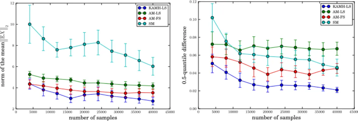
We next evaluate MCMC Kameleon on a number of artificial targets with high degrees of non-linearity. In these examples, exact quantile regions of the targets can be computed analytically, so we can directly assess perfor-mance without the need to estimate distribution distances on the basis of samples (i.e. by estimating MMD to the benchmark sample). We compute the following measures of performance (similarly as in Andrieu and Thoms [6] and Haario et al. [60]) based on the chain after burn-in: average accep-tance rate, norm of the empirical mean (the true mean is by construction zero for all targets), and the deviation of the empirical quantiles from the true quantiles.

Banana and flower target

In Haario et al. [60], the following family of non-linear target distribu-tions is considered. Let X _{∼ N}(0,Σ) be a multivariate normal in d_≥2 dimensions, withΣ=diag(v, 1, . . . , 1), which undergoes the transformation

Y∼ B(b,v). It is clear thatEY=0, and that B(y;b,v) =N(y1; 0,v)N(y2;b(y2₁−v), 1) d

∏

The second target distribution we consider is thed-dimensional flower target F(r0,A,ω,σ), with F(x;r0,A,ω,σ) = exp  ₋ q x₁2+x2₂₋r0−Acos(ωatan2(x2,x1)) 2σ2   × d

∏

This distribution concentrates around the r0-circle with a periodic pertur-bation (with amplitude Aand frequencyω) in the first two dimensions.

Results

We consider 8-dimensional target distributions: the moderately twisted B(0.03, 100) banana target (Figure 3.6, top) and the strongly twisted B(0.1, 100)banana target (Figure 3.6, middle) andF(10, 6, 6, 1)flower target (Figure 3.6, bottom).

The results show that MCMC Kameleon is superior to the competing samplers. Since the covariance of the proposal adapts to the local structure of the target at the current chain state, as illustrated in Figure 3.3, MCMC Kameleon does not suffer from wrongly scaled proposal distributions. The result is a significantly improved quantile performance in comparison to all competing samplers, as well as a comparable or superior accuracy in esti-mating the norm of the empirical mean. SMhas a significantly larger norm of the empirical mean, due to its purely random walk behaviour (e.g. the chain tends to get stuck in one part of the space, and is not able to traverse both tails of the banana target equally well). AMwith fixed scale has a low