Bank of Canada
Banque du Canada
Working Paper 2006-43 / Document de travail 2006-43
Efficient Hedging and Pricing of Equity-Linked
Life Insurance Contracts on Several Risky Assets
by
ISSN 1192-5434
Bank of Canada Working Paper 2006-43
November 2006
Efficient Hedging and Pricing of Equity-Linked
Life Insurance Contracts on Several Risky Assets
by
Alexander Melnikov
1and Yuliya Romanyuk
2 1Department of Mathematical and Statistical Sciences
University of Alberta
Edmonton, Alberta, Canada T6G 2G1
2
Financial Markets Department
Bank of Canada
Ottawa, Ontario, Canada K1A 0G9
The views expressed in this paper are those of the authors.
No responsibility for them should be attributed to the Bank of Canada.
iii
Contents
Acknowledgements. . . iv
Abstract/Résumé . . . v
1.
Introduction . . . 1
2.
Motivation . . . 2
3.
Literature Overview . . . 4
4.
Financial Setting . . . 6
5.
Insurance Setting . . . 9
6.
Eficient Hedging for Equity-Linked Life Insurance . . . 9
7.
Theoretical Results. . . 12
7.1
Example: applying efficient hedging . . . 17
8.
How Much Can You Lose? . . . 19
8.1
Example: maximal shortfall based on risk preference . . . 20
9.
Managing Financial and Insurance Risks . . . 21
9.1
Example: minimizing the shortfall risk. . . 21
9.2
Example: fixing the level of shortfall risk . . . 23
10.
Future Direction . . . 24
References. . . 25
Appendix A. . . 29
Appendix B . . . 30
Appendix C . . . 40
Appendix D. . . 54
iv
Acknowledgements
The authors gratefully acknowledge the valuable input of Dr. Michael King and helpful editing
remarks of Glen Keenleyside from the Bank of Canada. This paper was partially supported by
NSERC (Project 261855) and the University of Alberta (Project G021100024). The authors retain
any and all responsibility for errors, omissions, and inconsistencies that may appear in this work.
v
Abstract
The authors use the efficient hedging methodology for optimal pricing and hedging of
equity-linked life insurance contracts whose payoff depends on the performance of several risky assets.
In particular, they consider a policy that pays the maximum of the values of n risky assets at some
maturity date T, provided that the policyholder survives to T. Such contracts incorporate financial
risk, which stems from the uncertainty about future prices of the underlying financial assets, and
insurance risk, which arises from the policyholder’s mortality. The authors show how efficient
hedging can be used to minimize expected losses from imperfect hedging under a particular risk
preference of the hedger. They also prove a probabilistic result, which allows one to calculate
analytic pricing formulas for equity-linked payoffs with n risky assets. To illustrate its use,
explicit formulas are derived for optimal prices and expected hedging losses for payoffs with two
risky assets. Numerical examples highlighting the implications of efficient hedging for the
management of financial and insurance risks of equity-linked life insurance policies are also
provided.
JEL classification: G10, G12, D81
Bank classification: Financial markets
Résumé
Les auteurs emploient la méthode de couverture efficiente pour tarifer et couvrir de manière
optimale des contrats d’assurance vie indexés sur actions et dont le rendement dépend du
comportement d’un nombre n d’actifs risqués. Leur analyse porte en particulier sur le cas d’une
police qui verse à son titulaire, s’il est encore en vie à la date d’échéance T du contrat, une somme
égale à la plus élevée des valeurs prises par les n actifs risqués. Les polices de ce type comportent
autant un risque financier, découlant de l’incertitude entourant l’évolution du prix des actifs
sous-jacents, qu’un risque d’assurance, associé à la longévité du titulaire. Les auteurs montrent que la
méthode de couverture efficiente peut servir à minimiser l’espérance des pertes résultant d’une
couverture imparfaite, et ce, selon la propension au risque de l’opérateur en couverture. Ils
démontrent aussi un résultat probabiliste sur lequel peut s’appuyer le calcul des formules
analytiques servant à l’évaluation de la somme qui reviendra au titulaire de la police étant donné
un nombre n d’actifs risqués. Afin d’illustrer l’utilité de la méthode, les auteurs déduisent des
formules explicites permettant d’établir les prix optimaux et les pertes de couverture attendues
dans le cas où n est égal à deux. D’autres illustrations chiffrées sont données, afin de mettre en
vi
lumière les diverses applications de la méthode de couverture efficiente dans la gestion du risque
financier et du risque d’assurance propres aux contrats d’assurance vie indexés sur actions.
Classification JEL : G10, G12, D81
1. Introduction
Equity-linked insurance contracts have been studied since the middle of the 1970s. The payoff of such policies depends on two factors: the value of some underlying financial instrument(s) (hence the term equity-linked), and some insurance-type event in the life of the owner of the contract (death, retirement, survival to a certain date, etc.). As such, the payoff contains both financial and insurance risk elements, which have to be priced so that the resulting premium is fair to both the seller and the buyer of the contract. The famous results of Black and Scholes (1973) and Merton (1973) tell us that, in an idealized market setting, as long as the seller receives a price equal to the expectation under the risk-neutral probability measure of the discounted payoff, the seller can hedge this payoff perfectly – with probability of successful hedging equal to 1. Perfect hedging relies on the ability to trade the financial asset(s) underlying the payoff and the option itself so as to offset any movement in the values of the underlying asset(s) and the option. However, mortality risk cannot be offset in the same manner, since mortality is not (yet) traded, which makes the insurance market incomplete and renders perfect hedging of equity-linked life insurance contracts impossible (see section 5 for more details).
The goal of this paper is to illustrate how to apply efficient hedging to minimize the shortfall risk when dealing with equity-linked life insurance contracts written on several risky assets. The shortfall risk is defined as the expectation of the potential loss from the imperfect hedging strategy, weighted by some loss function reflecting the hedger’s risk preferences. In this paper, the terms ‘risk preference’ and ‘loss function’ refer to the attitude of the hedger (the insurance firm underwriting the policy) toward financial market risk. We do not discuss general risk preferences of market participants in the context of economic equilibrium. Rather, we consider whether the company selling an equity-linked policy is risk-averse, risk-indifferent, or possibly a risk-taker. Such an approach is taken in Foellmer and Leukert (2000), who develop the efficient hedging methodology in a mathematical finance-type context of optimal hedging under budget constraints. Building on the work of Kirch and Melnikov (2005), we extend the application of efficient hedging in the insurance context, showing that this method is a powerful tool that allows for many quantitative risk management possibilities, while at the same time being computationally practical, understandable, and justifiable not only to academics, but also to practitioners in the insurance industry.
We consider a single-premium equity-linked life insurance contract that enables its holder to receive the greater of the values of several risky assets (such as stocks) at the maturity of the contract, provided the policyholder survives to this date. We prove an interesting probabilistic result, which we refer to as the multi-asset theorem, that allows us to derive explicit pricing formulas for payoffs involving nrisky assets. We show how to apply the theorem in the context of the efficient hedging of payoffs on two risky assets by calculating formulas for optimal prices and maximal expected losses resulting from imperfect hedging for each of the risk-preference cases. In this, we extend the work of Melnikov and Romaniuk (2006)1 from a budget-constrainted investor utilizing quantile hedging for a contract with a single risky asset to a multi-asset Black-Scholes-Merton-type setting. We use historical values of the Dow Jones Industrial Average and Russell 2000 stock indexes to show how a company that sells an equity-linked contract on these indexes can assess, quantify, and hedge the resulting financial and insurance risk components based on a given risk preference. The significance of risk preferences on optimal hedging strategies is also illustrated numerically. The paper is structured as follows. Section 2 motivates the question of optimal pricing of equity-linked 1Note that the alternative spelling of Romanyuk is Romaniuk.
insurance in general, the particular payoff under consideration, and the choice of hedging methodology. Then we review briefly the existing literature on the pricing of equity-linked insurance and hedging of payoffs on multiple risky assets (section 3), and explain our paper’s contribution. In sections 4 and 5 we discuss the financial and the insurance market settings. In section 6 we present the formal set-up of the problem in the context of pricing of equity-linked life insurance contracts via efficient hedging.
We present the multi-asset theorem and the formulas for optimal prices and shortfall risk amounts for each of the risk-preference cases of the hedger in section 7. We illustrate theoretical results on the use of efficient hedging in general, when the investor is unable or unwilling to put up the entire amount needed for a perfect hedge. In section 8 we expand this topic by looking at maximal expected losses that the investor could bear based on the investor’s risk preference theoretically, and provide a numerical example. In section 9 we examine risk management strategies that measure and balance financial and insurance risk elements when efficient hedging is applied to price equity-linked life insurance contracts. Section 10 concludes with suggestions for future work. The proofs of theoretical results are included in appendixes.
2. Motivation
The insurance industry has grown at a tremendous pace in the past decade, especially with the devel-opment of new markets in Europe and Asia. Equity-linked (also known as ‘index-linked’) contracts, and contracts paying one unit of some risky asset (‘unit-linked’), have been especially successful. For example, in discussing world insurance growth in 1997, Swiss Re reported high growth in the life insurance business in Europe, North America, and the emerging markets in Western Europe, noting that the high growth rates were spurred in particular by dynamic business in unit-linked and index-linked insurance products (Swiss Re 1997). The National Association for Variable Annuities cited that, in the United States, the total industry sales of equity-indexed annuities grew from 0.2 to 12.6 billion dollars between 1995 and 2003 (NAVA 2004). Additionally, the Spanish Institute for Foreign Trade reported that, in Spain in 2000, the greatest growth occurred in unit-linked insurance products: 81 per cent compared with 21 per cent in other types (Spanish Institute for Foreign Trade 2002). Winterthur Life achieved a strong and remarkable growth in unit-linked business in Hong Kong in 2003, and launched markets for unit-linked insurance in 2001 and 2002 in Japan and Taiwan, respectively (Winterthur Life 2004). The Canadian market for seg-regated funds2 has also been quite successful, raising around 60 billion dollars in assets in 1999 (Hardy 2003).
Equity-linked and unit-linked businesses incorporate a wide variety of products, including variable annuities (United States), unit-linked insurance contracts (United Kingdom), equity-indexed annuities (United States), and segregated funds (Canada). The payoff on the maximum of several risky assets is embedded in some form in most products mentioned above. For example, in its simplest form, the payoff on the maximum of the values of a risky asset and a deterministic guarantee is incorporated in segregated funds and indexed universal life insurance, where premiums earn interest based on the performance of some risky fund but the insurance firm also guarantees a minimum rate of return. This payoff is also studied widely in the literature, for example, as an ‘asset-value guarantee’ (Brennan and Schwartz 1976, 1979; Boyle and Schwartz 1977), or ‘minimum death or maturity guarantee’ (Bacinello and Ortu 1993; Aase and Persson 1994). The payoff on the maximum of several risky assets is embedded in variable universal life products and segregated funds, where the premiums can be invested in one of the available risky funds,
and the investor can generally switch premiums to a better (more profitable) fund at certain dates. Since the payoffs considered in this paper are building blocks for a variety of equity-linked products, there is value to knowing how to price them properly.
Due to the rapid growth of equity-linked business, it is important to address the question of ‘correct’ pricing of equity-linked products in general. From the perspective of the insurance industry, the effects of failing to adopt adequate pricing and risk management models can be devastating. If the company overestimates and overprices its risks, the consumer will bear the financial burden of excessive insurance premiums, which may lead to government inquiries and regulation. If, on the other hand, the company undervalues its risks, it may face substantial losses and lose the confidence of investors and shareholders. In a stable and efficient economy, it is desirable to have all firms operating optimally in some sense; for example, without the risk of large losses or even bankruptcy. If a big insurance firm defaults, the negative effects of this event could be felt by the financial markets and the national economy, as well as individuals, shareholders, and clients of the firm. Clearly, some of the events causing large losses to insurance companies cannot be predicted (natural disasters, terrorist activities, etc.). However, fluctuations in the prices of risky assets and mortality patterns can be analyzed quantitatively and qualitatively to help build proper pricing tools for insurance firms. Thus the question of finding hedging methodologies that can assess and value financial and insurance risks, and provide appropriate risk management strategies, is of great interest and significance from both theoretical and practical perspectives.
One of the impediments to risk pricing arises from the growing market demand for flexible and person-alized insurance products. To respond to this demand and compete with financial institutions, insurance firms quickly develop and advertise, along with traditional life and health insurance, comparative products for investment and wealth management (variable annuities, segregated funds, etc.). The latter instruments are attractive to investors, since they tend to have shorter maturities and more exposure to financial market risk than traditional insurance contracts. Moreover, the ‘assurance’ component (a guarantee of some sort paid upon the death of the investor or upon surival to the contract’s maturity), together with generous tax benefits of equity-linked products, make them very successful alternatives to traditional investment instruments.
Before examining the pricing of equity-linked insurance products in more detail, we review how insur-ance firms hedge these contracts currently, and discuss whether these methods are appropriate. Several general practices of insurance companies have been pointed out in the literature. For example, Bacinello (2001) notes that mortality risk is generally not included explicitly in the valuation of insurance policies. Instead, firms account for this risk by using ‘safety-loaded’ life tables where survival probabilities are ‘loaded’ to reflect mortality/survival risks. Dahl (2004) states that, traditionally, insurance firms calculate premiums and reserves based on deterministic mortality and interest rates, and that to compensate for this, firms overprice financial and insurance risks, which results in higher than necessary premiums as well as room for error in estimating proper mortality and interest rates.
To illustrate how such ‘actuarial judgment’ may fail, Hardy (2003) brings up the case of Equitable Life (a large mutual company in the United Kingdom). In the 1980s, U.K. interest rates were higher than 10 per cent, and Equitable Life issued many contracts with guaranteed annuity options, in which the guarantees would move into the money only if interest rates fell below 6.5 per cent. Relying on their personal judgment, actuaries at Equitable Life believed that rates would never fall below 6.5 per cent. However, in the 1990s interest rates did fall below 6.5 per cent and the policies were cashed in, generating
such large guarantee liabilities that Equitable Life was forced to close to new business.
In this setting, one may argue that life insurance firms could buy options to manage the risks they carry from reinsurance companies. In this way, life insurance firms could insure their own risks. While reinsurance companies have been selling options that could be used to manage risks inherent in equity-linked contracts, the prices of these options have been such that life insurance firms selling the original equity-linked policies would be losing substantial portions of their expected profits. On top of that, insurance firms would be undertaking another risk – the risk of default of the reinsurer. Moreover, in some markets (such as segregated funds in Canada), reinsurance companies are becoming more and more reluctant to provide reinsurance at prices that are acceptable to insurance firms (Hardy 2003).
The International Accounting Standards Board (IASB) has highlighted the problem of improper pricing of financial and insurance risks (Biffis 2005). The IASB recognizes that mortality risk cannot be ignored in actuarial calculations and recommends that firms price both financial and insurance risks explicitly. The efficient hedging approach, discussed in this paper, allows the insurance firm to price the risks arising from volatility in the prices of risky assetsand mortality fluctuations. Also, the firm is able to choose and control its desired risk exposure for both financial and insurance risk elements. Efficient hedging is intuitive, since the minimization of potential losses is an obvious and natural criterion for risk management, and flexible, since it enables the hedger to incorporate risk preferences when pricing equity-linked policies. Finally, it allows users to derive explicit formulas for the premiums of contracts in consideration. While numerical solutions can be found to many problems arising in finance, it is still desirable to have closed-form solutions to these problems.3
3. Literature Overview
The topic of pricing of equity-linked insurance contracts became popular soon after the celebrated papers by Black and Scholes (1973) and Merton (1973) on the valuation of call options. Since equity-linked contracts incorporate both financial and insurance risk elements, perfect hedging in the sense of Black and Scholes (1973) and Merton (1973) does not work: the mortality risk of the option holder cannot be offset by trading in the insurance market, since mortality is not a traded asset.4 This section reviews some of the research on the pricing of risks entailed in equity-linked insurance products.5
Early contributions to the pricing of equity-linked insurance include Brennan and Schwartz (1976, 1979), Boyle and Schwartz (1977), and Delbaen (1986); among later authors on this topic are Bacinello and Ortu (1993), Aase and Persson (1994), Ekern and Persson (1996), Boyle and Hardy (1997), and Bacinello (2001). Note that most of these papers do not price financial and insurance risks explicitly. For example, Ekern and Persson (1996) calculate premiums for a large variety of equity-linked contracts, including those with payoffs where the contract owner chooses the larger of the values of two risky assets (and possibly a guaranteed amount) at the maturity of the contract, similar to the payoffs considered here. But the authors disregard mortality risk, calling it “unsystematic risk,” for which “the insurer does not receive any compensation.” The justification provided is the traditional argument that mortality risk can
3
As noted in Musiela and Zariphopoulou (2004), very few existing optimization-type approaches to optimal pricing of equity-linked insurance have produced explicit formulas that are intuitive and convey the idea behind the methodology.
4
However, it appears that a market for mortality is slowly developing. Special thanks to the anonymous referee of Melnikov and Romaniuk (2006) for this interesting and useful observation.
be eliminated by selling a large number of equity-linked contracts. Note, however, that pooling mechanisms do not seem to work.6
Another method for the valuation of equity-linked contracts stems from the utility-based indifference pricing approach, introduced by Hodges and Neuberger (1989) in the context of incomplete markets due to transaction costs. Here, the premium for the contract is calculated in such a way as to make the hedger (the insurance company, in our case) indifferent between including and not including a specified number of contracts in their portfolio. The method is extended to equity-linked insurance by Young and Zariphopoulou (2002a,b), who look at utility-based pricing when insurance risks are independent of the underlying financial asset (as in the setting considered in this paper), and Young (2003), who considers the situation where death benefits payable to the policyholder depend on the value evolution of the underlying financial asset.
Moeller (1998, 2001) incorporates financial and group mortality risk and determines the optimal hedging strategy as the one minimizing squared errors in future costs of the strategy. Our paper uses the efficient hedging methodology, whose goal is to minimize the expected losses of the hedger. This approach and the related concept of quantile hedging, where the probability of successful hedging is maximized, were developed by Foellmer and Leukert (1999, 2000) without the context of pricing and hedging of equity-linked contracts.7 A number of papers adapt quantile and efficient hedging to the insurance setting to price equity-linked contracts (Krutchenko and Melnikov 2001; Melnikov 2004a,b; Melnikov and Skornyakova 2005; Kirch and Melnikov 2005; Melnikov, Romaniuk, and Skornyakova 2005; Melnikov and Romaniuk 2006). Our work extends the research in the above contributions, where payoffs include one or two risky assets, by studying the application of efficient hedging in a more general financial setting withnrisky assets, whose returns are modelled by correlated Wiener processes. We also add to the existing results by examining quantitatively and qualitatively the maximal expected losses resulting from imperfect hedging based on the risk preference of the hedger.
European-type contracts with payoffs involving several risky assets have been studied by Margrabe (1978), who calculates the perfect hedging price of an option to exchange one risky asset for another (see also Davis 2002), and Stulz (1982), who derives analytical formulas for prices of European call and put options on the minimum or maximum of two risky assets in the classical Black-Scholes-Merton-type setting. Johnson (1987) generalizes the latter result to payoffs withnrisky assets using a change of numeraire technique, the characteristics of call/put options, and the lognormal properties of the underlying assets. Boyle and Tse (1990) present a fast and accurate approximation algorithm to value options on the maximum or minimum of several assets. Boyle and Lin (1997) obtain upper bounds for prices of call options on several assets without making any assumptions about the probability distribution of these assets. Laamanen (2000) further extends the result of Johnson (1987) to the payoffs on m best of n risky assets by utilizing a recursive approach in pricing calculations. We will derive a more general probabilistic-type result that allows us to value not only payoffs with several assets, but also to calculate directly expectations resulting from such payoffs being contingent upon other events; for example, when using efficient hedging to price equity-linked life insurance contracts.
6As indicated by the anonymous referee of Melnikov and Romaniuk (2006). 7
Related contributions include Spivak and Cvitanic (1999), Cvitanic and Karatzas (1999), Cvitanic (2000), Nakano (2004), and Kirch and Runggaldier (2004).
4. Financial Setting
We work in a financial market with an interest rate r >0, a riskless asset (a bank account, for instance)
B = (Bt)t∈[0,T], and risky assetsSi = (Sti)t∈[0,T],i= 1, . . . , nwith price evolutions
dBt = rBtdt ⇔ Bt=B0ert, B0 := 1; dSti = Sti(µidt+σidWti) ⇔ Sti=S0ie µi− σ2i 2 t+σiWti , (1)
where the constantsµi ∈R, σi>0 are the return and the volatility of the instantaneous return dS i Si of the risky assetSi. We model dSSii by correlated Wiener processesWi= (Wti)t∈[0,T]with the variance-covariance
matrix Ln: Ln = σ2 1 · · · σ1σnρ1n .. . . .. ... σ1σnρ1n · · · σ2n . (2)
ObviouslyLnis symmetric. We make the standard assumptions thatLnis invertible and thatρ2ij <1, i6=j; that is, the risks underlying the assets cannot be perfectly (positively or negatively) correlated. All processes are given on a standard stochastic basis (Ω,F,F = (Ft)t∈[0,T], P) and are adapted to the filtration F,
generated by Wi.
Define atrading strategy, orportfolio, as a predictable process π such that
π = (πt)t∈[0,T]= (βt, γt1, . . . , γnt)t∈[0,T]. (3)
Here, β represents the money invested in the riskless asset, B, and γti is the number of shares of Sti held in the portfolio at the instant of time t. The capital of π (also referred to as thewealth generated by π) is given by
Vtπ = βtBt+γt1St1+· · ·+γtnStn. (4) The strategies whose discounted capital satisfies
Vπ t Bt =V0π+ n X i=1 Z t 0 γuid Si u Bu (5)
are called self-financing. Only self-financing strategies that generate non-negative wealth are admissible. As is typical in such a setting, we assume that it is possible to trade in the financial market without any frictions (all assets are perfectly divisible, there are no transaction costs, there are no restrictions on lending/borrowing, etc.), and that the market admits no arbitrage opportunities.
From option pricing theory, we know that in the complete case, the equivalent martingale measure P∗
is unique (see, for example, Melnikov, Volkov, and Nechaev 2002). Consider a contingent claim whose payoff is anFT-measurable non-negative random variableH satisfyingH∈L1(P∗). In a complete market, the payoff H can be hedged perfectly; that is, there exists a unique (admissible) hedging strategy with (minimal) costV0 such that
In other words, the wealth generated by the perfect hedge will be sufficient to cover the liability of the option writer with probability 1. We also know that the cost of this perfect hedge is given by
V0=H0 =E∗(He−rT). (7)
Above, and for the remainder of the paper, e will denote the exponent function, T the maturity of the contract, and E and E∗ the expectations with respect to the subjective (‘real-world’) and objective (risk-neutral, or equivalent martingale) measures P and P∗, respectively.
In our setting, the financial payoff allows the policyholder to receive the largest of the values ofnrisky assets at maturity:
H = max{ST1, . . . , STn}. (8) The perfect hedging price of this payoff is calculated according to (7), and we know how to derive the explicit formula for the price (see, for instance, Johnson 1987 or Romanyuk 2006). However, problems arise when H is payable only upon the survival of the policyholder until the policy’s expiration atT. As we will see shortly, such a condition lowers the initial (perfect hedging) price of H, creating a positive probability that the writer of the policy will default on the payment of H.
Before we discuss the insurance setting, let us briefly remark on the financial market setting in the case of two risky assets, since we will illustrate the use of the multi-asset theorem in the process of deriving optimal prices for the payoff on the maximum of two assets.
In the financial market setting with two risky assets, the fluctuations in asset returns are modelled by two Wiener processes W1 and W2 with correlation ρ underP. Because there are two assets to trade and two sources of risk (W1, W2), the financial market is complete (and arbitrage-free; see Melnikov, Volkov,
and Nechaev 2002). Therefore, there exists a unique risk-neutral probability measure P∗ with density Z
such that
Zt=
dP∗
dP |Ft, t∈[0, T]. (9) Using the general methodology for finding martingale measures (presented in Melnikov and Shiryaev 1996, and Melnikov, Volkov, and Nechaev 2002), we calculate the expression for Z explicitly (for derivation details, see Appendix A):
Zt = eφ1W 1 t+φ2Wt2− σ2φ 2 t, (10) where φ1 = r(σ2−σ1ρ) +ρµ2σ1−µ1σ2 σ1σ2(1−ρ2) , φ2 = r(σ1−σ2ρ) +ρµ1σ2−µ2σ1 σ1σ2(1−ρ2) , (11) and σ2φ=φ21+φ22+ 2ρφ1φ2. (12)
UnderP∗, the evolutions ofS1 and S2 can be rewritten as
dSti = Sti(rdt+σidWti∗) ⇔ Sti =S0ie r−σ2i 2 t+σiWti∗ , i= 1,2. (13)
Here, Wi∗= (Wti∗)t∈[0,T] are Wiener processes with correlationρ underP∗ that satisfy Wti∗ =Wti+θit, (14) with θi = µi−r σi . (15)
It follows that discounted S1 and S2 are martingales with respect to P∗. Using (10) and (14), we rewrite the expression forZ under P∗:
Zt=e φ1Wt1∗+φ2Wt2∗− σφ2 2 +φ1θ1+φ2θ2 ! t . (16)
Note that in derivations of pricing formulas, we will use the formulas for Si andZ under both the original (P) and the risk-neutral (P∗) probability measures.
Next, consider the parameterθi given in (15). In the financial literature, θis referred to as the market price of risk: this is the additional ‘reward’ per unit volatility investors receive to compensate them for the willingness to bear risk when putting money in risky, as opposed to riskless, assets. We require that
θi >0 ⇔ µi > r; (17) otherwise, an arbitrage strategy with zero initial outlay and positive expected return could be constructed (short a stock and invest the proceeds in a bond, then use the principal and interest from the bond to buy back the stock).
In the setting with two risky assets, the payoff takes the form
H = max{ST1, ST2}=ST1I{S1 T≥S 2 T}+S 2 TI{S1 T<S 2 T}. (18)
As such, H is the payoff for a purely financial contract, whose fair price is determined uniquely by (7). The explicit formula for the fair price (see, for example, Stulz 1982) is given by
H0 = E∗ max{ST1, ST2}e−rT
=S01·Ψ1(˜y1) +S02·Ψ1(˜y2), (19)
where Ψ1 denotes a one-dimensional cumulative normal distribution: foru∼N(0,1),
Ψ1(c) = Z c −∞ e−u2/2 √ 2π du. (20)
The constants ˜y1,y˜2 are defined as
˜ y1 = ln S1 0 S2 0 +σ22T σ√T , y˜2 = ln S2 0 S1 0 +σ22T σ√T , (21) and σ2 = σ12+σ22−2ρσ1σ2. (22)
5. Insurance Setting
Let a random variable τ(x) on a probability space ( ¯Ω,F¯,P¯) denote the remaining lifetime of a person of current age x. We make the standard assumption that the insurance risk arising from clients’ mortality and the financial market risk have no (or very minimal) effect on each other, and hence the two probability measures P and ¯P are independent (Luciano and Vigna 2005).
Term insurance products are types of policies whose payoff occurs before the maturity of the policy. For example, one could buy a 20-year policy paying 10,000 Canadian dollars in case the death of the policyholder occurs within 20 years from the date of purchase. On the other hand, the payoff of life insurance products occurs on or after the maturity of the policy, as long as some prespecified event did not happen prior to the maturity date. We work with a single-premium equity-linked life insurance policy where the policyholder receives the payoffH given by (8), provided that the policyholder is alive to collect that payoff. That is, we consider the payoff ¯H:
¯
H=H·I{τ(x)>T}, (23) whereI refers to the indicator function that equals 1 if the insured survives toT ({τ(x)> T}), or 0 if the insured dies before T. The fair premiumU0 for a contract with such a payoff is
U0 = E∗×E He¯ −rTI{τ(x)>T}
= E∗ He−rT ¯
P{τ(x)> T}
= E∗ He−rTTpx, (24) where Tpx = ¯P{τ(x) > T} denotes the probability of a life aged x survivingT more years, andE∗ ×E¯ denotes the expectation with respect to the product measure P∗×P¯.
Notice that the mortality of the insured client (as reflected by the client’s survival probability Tpx) makes it impossible for the insurance firm writing the contract to hedge its payoff with probability 1:
0<Tpx <1 ⇒ U0< H0 =E∗ He−rT
. (25)
As mentioned previously, since mortality is not traded directly, it is not possible to hedge mortality risk as one hedges the risk associated with trading financial options, by taking positions in the underlying risky asset(s). Thus the insurance market is incomplete.
6. Efficient Hedging for Equity-Linked Life Insurance
In the situation when the quantity U0 (24), collected by the firm from the sale of the equity-linked life
insurance contract with payoff (23), is strictly less than the amount H0, necessary to hedge the payoff
perfectly, the firm faces the risk of default. To reduce this risk, the company must find some appropriate imperfect hedging technique that optimizes hedging outcomes, given constraints on initial capital available for hedging. In this section, we show how efficient hedging can be applied in this situation.8
8
In this paper, we give only the general idea behind the efficient hedging methodology and refer the reader to Foellmer and Leukert (2000) and Romanyuk (2006) for details on the method and its extension to our setting.
The purpose of efficient hedging is to minimize the potential losses, weighted by the hedger’s risk preference, from imperfect hedging. More specifically, efficient hedging aims at finding an admissible hedging strategy π∗ that minimizes the shortfall risk:
El((H−VTπ∗)+)= min π E l((H−V π T)+) with V0≤U0< H0. (26)
Here,ldenotes the loss function that reflects the investor’s (hedger’s) risk preference. Foellmer and Leukert (2000) work with power loss functionl(x) =xp,p >0, where the different values forpreflect the particular view toward risk. Note that p >1 implies that the investor is risk-averse: the larger the investor’s losses, the more the investor ‘feels’ them. The case p = 1 corresponds to risk indifference, where the investor perceives losses one-for-one with the dollar amount lost. If 0 < p < 1, the investor is a risk-taker: the investor cares less about larger losses than smaller ones. While this last attitude may seem irrational, we can think of this type of investor as an addicted gambler, who finds it more and more difficult to stop playing as their losses get larger.
Foellmer and Leukert (2000) show that the solution to the problem in (26) is the perfect hedgeπ∗ for the modified contingent claim
H∗ =ϕ∗H, (27) where ϕ∗ is determined9 as ϕ∗ = 1− I a ∗e−rTZ T H ∧1 ! for p >1, (28)
with I = (l0)−1 denoting the inverse of the derivative of the loss functionl,
ϕ∗=I{1>a∗e−rTH1−pZ
T} for 0< p <1, (29) and, finally,
ϕ∗=I{1>a∗e−rTZ
T} for p= 1. (30)
The inequalities in (26) reflect the fact that the investor is budget constrained, U0 < H0 (H0 =
E∗(He−rT) is the amount needed for a perfect hedge), and the requirement that the initial cost V0 of the
optimal hedging strategy must not be greater than the amount available to the hedger, V0 ≤ U0. Note
that the cost of the optimal hedging strategy π∗ (the one minimizing the shortfall risk for payoffH under the budget constraint U0) is the price of the perfect hedge for the modified contingent claim H∗, given by
U0 (Foellmer and Leukert 2000).
It is worthwhile to highlight the elegance of the efficient hedging approach in the situation with financing constraints. The constraint on the initial hedging capital may arise due to some external factor beyond the hedger’s control (such as mortality risk in equity-linked life insurance contracts), or a circumstance within the decision-making power of the hedger (the hedger may be unwilling to put up the entire amount required for perfect hedging and be prepared to take some risk as a trade-off for offering the contract at a
9
The expressions forϕ∗correspond to those denoted ˜ϕin Foellmer and Leukert (2000) forr= 0. We work with a non-zero interest rate. Please see Romanyuk (2006) for more information on how to adapt the results of Foellmer and Leukert (2000) to our setting in particular, and to the pricing of equity-linked life insurance contracts in general.
lower price). In either case, the hedger can solve the problem of insufficient initial capital by minimizing the shortfall risk as follows. The hedger should invest U0 into the (optimal) strategy π∗, which perfectly
hedges the modified contingent claim H∗, and the desired optimization goal will be achieved. Of course, one must take care to select theH∗ and π∗ that correspond to the appropriate risk preference. We believe that this risk management approach is easy to understand and thus is likely to be implemented.
In section 7.1, we will illustrate the situation where the investor cannot provide the entire amount of
H0 required for a perfect hedge and is ready to accept some shortfall risk. Since shortfall is an amount
that could be lost due to imperfect hedging, it is expressed in dollar terms. We will show the possible risk management strategies based on two different perspectives of the hedger. First, we will calculate the level of shortfall risk if the hedger is willing to invest U0, taken as a percentage ofH0, into the optimal hedge.
Second, we will illustrate how much initial capital U0 is required if the hedger wants to keep shortfall at
some acceptable level, specified beforehand.
We can extend our study of efficient hedging far beyond purely financial risk management considera-tions: the flexibility of this hedging methodology makes it an excellent risk management tool for insurance applications, particularly in the case of equity-linked life insurance products. Let us discuss this point in more detail. On the one hand, we showed in (24) that U0 is the fair premium for an equity-linked life
insurance contract with payoff ¯H (23). On the other hand, the main result of efficient hedging tells us that the budget constraint (U0 in our case) is also the cost of the optimal strategyπ∗, which perfectly hedges
the modified contingent claim H∗ given by (27). Based on this, we obtain the following equalities for the price of the equity-linked life insurance contract in consideration:
U0 = E∗×E¯( ¯He−rT) =E∗(H∗e−rT) (31)
= E∗(He−rT)Tpx=E∗(H∗e−rT), from which we can express the survival probability of the policyholder as
Tpx =
E∗(H∗)
E∗(H) . (32)
The term E∗(He−rT) above is known ((19) for the payoff with two assets; for nassets, see Johnson 1987): it is simply the cost of the perfect hedge for H (7).
Equations (31) and (32) are essential to the subsequent risk management analysis of efficient hedging in insurance applications, since they give a quantitative connection between financial and insurance risk components. Such a connection allows the insurance firm to assess accurately the risks it bears, and to implement specific strategies to control these risks according to the preferred risk management approach. That is, the firm can either offer equity-linked contracts to any client and then, based on the fair price received from this client, minimize the shortfall risk, or the firm can set the acceptable amount of expected shortfall and then analyze clients for the contracts accordingly.
More specifically, using the first approach, the firm will derive the client’s survival probability Tpx based on the client’s known agexfrom life tables or some appropriate mortality model. Then the firm will find a∗ from (27) and (32), and proceed to compute the shortfall risk using (26). Note that the obtained value for the minimized shortfall may not fit the company’s desired risk profile. Alternatively, the firm can utilize equation (32) in reverse: first, choose some acceptable amount of shortfall, calculate a∗, and then find the survival probabilities Tpx of potential clients. Next, using life tables or an appropriate mortality
model, the ages of clients paying fair premiums (under the prescribed risk level) can be derived and risk management consequences analyzed in light of the firm’s risk preferences. We will illustrate both of these approaches in section 9.
7. Theoretical Results
In this section, we present the multi-asset theorem, which is used in computing pricing and shortfall formulas for equity-linked life insurance contracts with payoff ¯H (23). As a particular application of the theorem, we give explicit formulas for the fair premium, shortfall risk amount, and maximal expected shortfall for each of the three risk attitudes of the hedger (risk aversion, risk taking, and risk indifference). Recall that the shortfall risk amount is the expected loss from the imperfect hedge that results from the constraintU0 on the initial hedging capital available to the investor; this shortfall risk is minimized when
U0 is invested into the optimal hedge π∗ (see discussion before (31)).
Based on equations (8), (24), and (31), in order to find, for instance, the fair premiumU0 for the case
of risk indifference (see (30)), we need to evaluate the following expression:
U0 = E∗ max{ST1, ST2, . . . , STn} erT ϕ ∗ (33) = E∗ ST1 erTI{1>a∗e−rTZ T}I{ST1≥ST2}I{ST1≥ST3}· · ·I{S1T≥STn} +E∗ ST2 erTI{1>a∗e−rTZT}I{S2T>ST1}I{ST2≥S3T}· · ·I{ST2≥SnT} +· · ·+E∗ SnT erTI{1>a∗e−rTZT}I{SnT>ST1}I{STn>ST2}· · ·I{Sn T>S n−1 T } .
BecauseSi andZ depend on normally distributed Wiener processesWi, we can represent the expectations above as
E∗ e−zI{x1<X1}· · ·I{xn<Xn}
, (34)
where X1, . . . , Xn are constants, andz, x1, . . . , xn are normally distributed random variables with appro-priately determined means, variances, and correlations. To compute such expectations explicitly, we prove the following theorem.
Theorem 1: multi-asset theorem
Let xi ∼N(µi, σ2i), i= 1, . . . , n and z∼N(µz, σ2z) ben+ 1 normally distributed random variables with a variance-covariance matrix Rn+1 given by
Rn+1 = σ12 · · · σ1σzρ1z .. . . .. ... σ1σzρ1z · · · σz2 . (35)
Then, for some given constants Xi, E e−zI{x1<X1}· · ·I{xn<Xn} = e− µz− σ2z 2 ·Ψn( ˆX1, . . . ,Xˆn), (36) ˆ Xi = Xi−µi σi +σzρiz.
In the formulation of the theorem, we refer to xn+1 as z, to distinguish the fact that the n+ 1 random
variable is in the exponent. Also, Ψn, n > 1, denotes the n-dimensional cumulative normal distribution (see below) of nrandom variables with mean 0, variance 1, and the correlation matrix
˜ Rn = 1 · · · ρ1n .. . . .. ... ρ1n · · · 1 , (37)
with the inverse ˜R−n1 = ˜An.
The general formula for the k-dimensional cumulative normal distribution of (k) random variables
yi ∼N(µi, σi2) with the variance-covariance matrix Dk is given by
Ψkgeneral(c1, . . . , ck) = 1 (2π)k/2|D k|1/2 Z c1 −∞ · · · Z ck −∞ e−12 Pk i=1 Pk j=1bij(yi−µi)(yj−µj)dy 1· · ·dyk, (38) Dk = σ12 · · · σ1σkρ1k .. . . .. ... σ1σkρ1k · · · σk2 , Bk=kbijkk=D −1 k .
Please note that, for the remainder of the paper (including the appendixes), Ψk, k > 1, without the subscript ‘general,’ will refer to the k-dimensional cumulative normal distribution of correlated random variables with mean 0 and variance 1.
Proof. See Appendix B.
Theorem 2: premiums and shortfall risk amounts
Suppose that an insurance firm has sold an equity-linked life insurance contract with payoff providing the maximum of two risky asset values upon the survival of the buyer until the maturity of the contract. Suppose further that the firm decides to use efficient hedging to minimize the shortfall risk.
Part I. The firm’s risk preference is risk aversion: for the loss function l(x) =xp,p >1. a. The fair premium for the contract is
U0 = S01·Ψ2(˜xA1,y˜1, ρ1A) +S02·Ψ2(˜xA2,y˜2, ρA2)
−M·
Ψ2(˜c1,y˜1c, ρA1) + Ψ2(˜c2,y˜2c, ρA2)
b. The shortfall risk amount is given by E l((H−VT)+) = N· Ψ2(¯c1,y¯c1, ρA1) + Ψ2(¯c2,y¯2c, ρA2) +(S01)pe µ1− σ12 2 T p+σ 2 1 2 T p 2 ·Ψ2(¯k1,y¯1k,−ρA1) +(S02)pe µ2− σ22 2 T p+σ 2 2 2 T p 2 ·Ψ2(¯k2,y¯2k,−ρA2). (40)
Part II. The firm’s risk preference is risk taking: for the loss functionl(x) =xp, 0< p <1. a. The fair premium for the contract is
U0 = S01·Ψ2(˜xT1,y˜1, ρT1) +S02·Ψ2(˜xT2,y˜2, ρT2). (41)
b. The shortfall risk amount is given by
E l((H−VT)+) = (S01)pe µ1− σ12 2 T p+σ 2 1 2 T p 2 · Ψ1(¯y1T)−Ψ2(¯xT1,y¯1T, ρT1) +(S02)pe µ2− σ22 2 T p+σ 2 2 2 T p 2 · Ψ1(¯y2T)−Ψ2(¯xT2,y¯T2, ρT2) . (42)
Part III.The firm’s risk preference is risk indifference: for the loss function l(x) =xp,p= 1. a. The fair premium for the contract is
U0 = S01·Ψ2(˜xI1,y˜1, ρI1) +S02·Ψ2(˜xI2,y˜2, ρI2). (43)
b. The shortfall risk amount is given by
E l((H−VT)+) = S01eµ1T · Ψ1(¯y1I)−Ψ2(¯xI1,y¯1I, ρI1) +S02eµ2T ·Ψ1(¯yI 2)−Ψ2(¯xI2,y¯2I, ρI2) . (44)
Above, Ψ2 denotes two-dimensional cumulative normal distribution (see (38)) with the corresponding correlations ρAi =ρTi = φj(σj −σiρ)−(φi−σi(p−1))(σi−σjρ) σEi σ , ρIi = φj(σj −σiρ)−φi(σi−σjρ) σφσ , (45) fori, j = 1,2.
The remaining constants are defined as M = a∗ p 1 p−1 · e σ2φT 2(p−1)2 e rT+ r+σ 2 φ 2 +φ1θ1+φ2θ2 ! T p−1 , (46) N = a∗ p p−p1 · e σ2φT p2 2(p−1)2 e r+ σ2 φ 2 ! T p p−1 , (47) ˜ xAi = ln (S0i)p−1ap∗ + pr+ σ2i 2 +σ 2 φ−σ 2 i 2 +φi(θi−σi) +φj(θj−ρσi) T σEi √T , (48) ˜ ci = ln (Si 0)p−1 p a∗ + pr−σ2i 2 +σ 2 φ+σ 2 i 2 − σφ2 p−1 +φi(θi+σi) +φj(θj+ρσi) T σEi √T , (49) ˜ yic = ln Si 0 Sj0 + σ2 j−σ2i 2 T+ [φi(σi−σjρ)−φj(σj−σiρ)]pT−1 σ√T , (50) ¯ ci = ln (S0i)p−1ap∗ + r+σ 2 φ 2 − σ2 φp p−1 + (p−1) µi−σ 2 i 2 +p(φiσi+φjσiρ) T σE i √ T , (51) ¯ yic = ln Si 0 S0j + µi−µj+ σ2 j−σ2i 2 + p p−1(φi(σi−σjρ)−φj(σj−σiρ)) T σ√T , (52) ¯ ki = lnap∗(S0i)1−p− r+σ 2 φ 2 + (p−1) µi− σ2 i 2 −p(φiσi+φjσiρ−σi2(p−1)) T σE i √ T , (53) ¯ yik = ln Si 0 Sj0 + µi−µj+ σ2 j−σ2i 2 +p(σi2−σiσjρ) T σ√T , (54)
˜ xTi = σ2 φ−σ2i 2 +φi(θi−σi) +φj(θj −ρσi) +p r+ σ2i 2 T −ln (S0i)1−pa∗ σE i √ T , (55) ¯ xTi = r+σ 2 φ 2 −(1−p) µi− σ2 i 2 −p(σ2i(1−p) +φiσi+φjσiρ) T−ln (S0i)1−pa∗ σiE√T , (56) ¯ yiT = ln Si 0 Sj0 + µi−µj+ σ2 j−σ2i 2 +p(σi2−σiσjρ) T σ√T , (57) ˜ xIi = r+σ 2 φ 2 +φi(θi−σi) +φj(θj−ρσi) T−ln (a∗) σφ √ T , (58) ¯ xIi = r+σ 2 φ 2 −φiσi−φjσiρ) T−ln (a∗) σφ √ T , (59) ¯ yIi = ln Si 0 Sj0 + h µi−µj+σ 2 2 i T σ√T , (60) (σEi )2 = σφ2+ (1−p)2σi2−2σi(1−p)θi. (61) Note that ˜yi are given in (21),φiin (11),θiin (15),σ in (22), andσφin (12). Also, the formulas for the premium and the shortfall risk for the cases of risk aversion and risk taking hold as long as the technical conditions ρ 6= θ1
θ2 and ρ 6= θ2
θ1 are satisfied, as explained in the proof of Theorem 2. The conditions are not restrictive in any way: the likelihood of having two risky assets with a correlation of the underlying Wiener processes being exactly equal to the ratio of θi is very small. However, in case this does happen, there are ways to deal with the situation (please see the proof for more details).
7.1 Example: applying efficient hedging
Let us demonstrate how an investor can use efficient hedging to deal with insufficient initial capital. We do not deal with an insurance risk element yet; that aspect of equity-linked life insurance contracts will be illustrated in section 9. For now, we focus on showing what risk management strategies are available to the hedger utilizing the efficient hedging technique under budget constraints.
To calculate the parameters for our model (µi, σi, ρ, i= 1,2), we use daily stock prices of the Russell 2000 (RUT-I) and Dow Jones Industrial Average (DJIA) indexes from 1 August 1997 to 31 July 2003. The data are taken from Yahoo! finance.10 The first index, RUT-I, reflects the performance of 2000 smaller firms in the United States, while the second, DJIA, represents 30 large and prestigious U.S. companies. The parameters are calculated using a standard approach in finance (see, for example, Hull 2005):
ln St+∆t St = µ−σ 2 2 ∆t+σ √ ∆tz, (62)
where z ∼N(0,1). In our case ∆t= 2521 , since we take the business year to have 252 days. We estimate the mean and the standard deviation of ln
S
t+∆t St
in a straightforward manner, and then multiply them by 252 and √252, respectively, to obtain annualized values. Note that we add to the annualized mean half of the estimated (annualized) variance to obtain µ.
The estimated parameters are as follows:
µ1 = 0.0482, µ2= 0.0419, σ1 = 0.2234, σ2 = 0.2093, ρ= 0.71.
We take the 31 July 2003 values of the indexes for the initial prices of the risky assets, correcting for the large difference between the two, so that
S01 = (9233.8/476.02)·476.02, S02= 9233.8.
For the estimate of the interest rate, we look at five-year nominal yields on U.S. treasury securities11 and take r= 0.04, or 4 per cent, which is close to the average of the yields in the early 2000s.
We consider a five-year contract with payoff max{S51, S52} and the situation where the seller of the contract is not able to collect (or is not willing to provide) the amount necessary to invest into the perfect hedging strategy. We calculate the perfect hedging price (19) and the price of the optimal hedging strategy as prescribed by efficient hedging ((43), (41), and (39)). We analyze two risk management approaches. First, we find the amounts of an expected shortfall ((44), (42), and (40)) for the different risk preferences based on the available level of initial capital, given as a percentage of the perfect hedging price. Second, we look at what levels of initial capital the investor requires to hedge the payoff with the desired level of shortfall risk. We take p= 1,p= 0.8, andp= 1.2 to describe the respective attitudes of risk indifference, risk taking, and risk aversion.
The results are summarized in Tables 1 and 2. Note that the perfect hedging price for the contract is US$10,587.54.
10Available online at<http://www.finance.yahoo.com>. 11
Table 1: Expected shortfall (amount and percentage of the perfect hedging price) based on selected levels of initial hedging capital (given as a percentage of the perfect hedging price) for risk indifference, risk taking, and risk aversion
Initial capital available Expected shortfall
p= 1.0 90 1,101.54 (10.40) 95 533.87 (5.04) 99 100.51 (0.95) p= 0.8 90 160.06 (1.51) 95 77.19 (0.07) 99 14.10 (0.01) p= 1.2 90 5,240.32 (49.50) 95 2,290.30 (21.63) 99 326.77 (3.09)
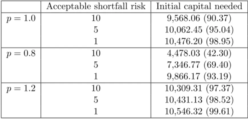
Table 2: Initial capital (amount and percentage of the perfect hedging price) required to maintain a selected shortfall risk level (given as a percentage of the perfect hedging price) for risk indifference, risk taking, and risk aversion
Acceptable shortfall risk Initial capital needed
p= 1.0 10 9,568.06 (90.37) 5 10,062.45 (95.04) 1 10,476.20 (98.95) p= 0.8 10 4,478.03 (42.30) 5 7,346.77 (69.40) 1 9,866.17 (93.19) p= 1.2 10 10,309.31 (97.37) 5 10,431.13 (98.52) 1 10,546.32 (99.61)
First, we observe some expected patterns across all risk-preference cases. The higher the initial capital provided by the investor for the optimal hedging strategy, the smaller is the shortfall amount (Table 1). Equivalently, the lower the shortfall risk acceptable to the investor, the greater is the amount of initial capital required for the optimal hedge (Table 2). Such results agree with our intuition about the short-fall/capital relationship, which will be examined in more detail in section 8.
Next, let us compare the values between the three risk-preference cases. Table 1 shows that, for the same given level of initial capital, the amount of expected shortfall will be perceived as less by a risk-taker and more by a risk-averse investor than the shortfall expected by a risk-indifferent investor. We take the risk-indifference case as the benchmark, since this shortfall amount is the actual expected dollar loss. For example, suppose that three investors can provide the initial capital of only 90 per cent of the amount required for the perfect hedge. The actual minimized expected loss in this situation is about 1,100 dollars; this is the amount a risk-indifferent investor would see as being lost due to insufficient initial capital. A risk-taker, providing the same dollar amount for the optimal hedge, would value the expected loss at
only 160 dollars; clearly, the risk-taker cares less about losing money than the risk-indifferent investor. A risk-averse investor, on the other hand, would ‘feel the pain’ much more sharply: for such an investor, the perceived loss from insufficient initial capital is valued at over 5,000 dollars (Table 1).
We observe a similar pattern in Table 2. To keep the level of acceptable shortfall risk at, say, 5 per cent, the risk-indifferent hedger would invest about US$10,000 into the optimal hedge. For the same shortfall risk, the risk-taker would give only US$7,300, while the risk-averse investor would pay about US$400 more than is required by the benchmark case of risk indifference. Again, this is due to the fact that the risk-taker feels losses less, and the risk-averse investor more, than the hedger who values losses based on actual dollar amounts.
Based on the foregoing discussion, let us think about the shortfall/capital relationship a little more. When the level of initial capital available for hedging approaches the perfect hedging price, the expected shortfall should approach zero. Equivalently, the smaller the level of shortfall risk acceptable to the hedger, the larger should be the capital required to invest in the optimal hedging strategy. These intuitive ideas are somewhat illustrated in Tables 1 and 2 and will be proved in Theorem 3 (section 8). But what happens to the expected shortfall for each risk attitude as the capital available for hedging becomes increasingly smaller? Intuitively, it seems correct to think that the expected shortfall should approach the expected (under the subjective probability measure P) full amount of the payoff in the case of risk indifference. A hedger who values losses one-for-one with actual dollar amounts should not expect to lose more or less than the payoff H, which has to be paid to the buyer of the contract at its maturity. But a risk-taking hedger, who cares less about losses, should value the maximal expected shortfall less (and a risk-averse investor more) than the risk-indifferent person. This is an interesting topic, and we will examine it in more detail in the next section.
8. How Much Can You Lose?
Following the discussion about maximal expected losses, let us see what happens to the shortfall risk as the initial amount available for hedging
a. approaches the perfect hedging price, or b. approaches zero.
We already gave the intuition behind the relation capital/shortfall. The aim of this section is to justify and quantify the idea that as initial capital approaches the perfect hedging price, the amount of shortfall goes to 0. And, as initial capital goes to 0, the shortfall risk increases to some boundary that depends on the risk preference of the hedger.
Theorem 3: maximal expected shortfall
Part I. The investor’s risk preference is risk aversion.
a. Whenever the initial capital of the optimal hedging strategy (39) approaches the perfect hedging price (19), the shortfall risk (40) goes to 0.
b. The shortfall risk approaches
max shortfallA = (S01)pe µ1− σ12 2 T p+σ 2 1 2 T p 2 ·Ψ1(¯yk1) + (S02)pe µ2− σ22 2 T p+σ 2 2 2 T p 2 ·Ψ1(¯y2k) (63)
whenever the initial hedging capital goes to 0. Note that ¯yik are given in (54).
Part II. The investor’s risk preference is risk taking.
a. Whenever the initial capital of the optimal hedging strategy (41) approaches the perfect hedging price (19), the shortfall risk (42) goes to 0.
b. The shortfall risk approaches
max shortfallT = (S01)pe µ1− σ21 2 T p+σ 2 1 2 T p2 ·Ψ1(¯y1T) + (S02)pe µ2− σ22 2 T p+σ 2 2 2 T p2 ·Ψ1(¯y2T) (64) whenever the initial hedging capital goes to 0. Note that ¯yiT are given in (57).
Part III.The investor’s risk preference is risk indifference.
a. Whenever the initial capital of the optimal hedging strategy (43) approaches the perfect hedging price (19), the shortfall risk (44) goes to 0.
b. The shortfall risk approaches
max shortfallI = S01eµ1T ·Ψ1(¯yI
1) +S02eµ2T ·Ψ1(¯y2I) (65)
whenever the initial hedging capital goes to 0. Note that ¯yiI are given in (60).
Proof. See Appendix D.
8.1 Example: maximal shortfall based on risk preference
Let us illustrate how the amounts of the maximal shortfall risk differ based on the risk preference of the hedger. We use the same data, estimates, and contract type as in the numerical example in section 7.1. Based on these numbers, we calculate that, in the case of risk indifference (p = 1), the largest expected shortfall is US$13,270.06. Table 3 provides the values for risk taking (0< p <1) and risk aversion (p >1).
Table 3: Values of maximal shortfall risk (dollar amounts) for various risk preferences of the investor
p, risk taking Max shortfall p, risk aversion Max shortfall 0.0001 1.00 1.0001 13,282.81 0.1 2.56 1.1 34,696.96 0.2 6.56 1.2 90,917.44 0.3 16.87 1.3 238.749.10 0.4 43.45 1.4 628,313.24 0.5 112.15 1.5 1,657,112.04 0.6 290.10 1.6 4,379,958.56 0.7 752.02 1.7 11,601,974.26 0.8 1,953.64 1.8 30,799,160.76 0.9 5,086.17 1.9 81,939,309.75 0.9999 13,270.06 2.0 218,470,861.00
First of all, note that, as p → 1, the values of the maximal expected shortfall for both risk aversion and risk taking approach the amount of the largest expected shortfall in the risk-indifference case, which is expected. When a risk-taking investor becomes more risk-averse, that investor begins to value potential losses higher. And, when risk aversion grows, the investor becomes increasingly sensitive to shortfall risk. These results agree with our intuition. It is interesting to observe that, when the level of risk aversion changes by 1 (from p = 1 to p = 2), the value of the potential loss increases by a factor of about 15,000 (that’s a lot!). Or, when risk-taking habits change from 1 to 0, the expected loss decreases by a factor of about 13,000. Such situations seem too extreme; in the real world, the risk attitudes of the majority of investors probably fall close to p= 1.
9. Managing Financial and Insurance Risks
In the numerical examples presented so far, we have ignored the element of insurance risk that arises due to the dependence of the payoff on the client’s survival to the maturity of the equity-linked contract. We have illustrated the situation where the initial capital available to the investor is smaller than the amount needed for a perfect hedge (for whatever reason). We have analyzed the resulting implications on the levels of shortfall risk per given amount of initial hedging capital (and vice versa: initial capital required per specified level of shortfall), as well as on maximal shortfall amounts depending on the investor’s risk preference.
Next we analyze the insurance component of optimal hedging under budget constraints, and illustrate how the mortality risk of the policyholder affects the risk management considerations for the seller of the policy. We study the situation where an insurance company sells a contract allowing its holder to choose the larger of two risky fund values at the expiration of the contract, provided that the client survives to that date to collect the payoff. Recall that the conditioning of the payoff on the client’s survival to the maturity of the contract reduces the fair premium of this contract, leaving the hedger (the insurance firm) with insufficient initial capital for a perfect hedge (section 6). Thus at each moment after the sale of the policy, the insurance firm is exposed to financial risk arising from market fluctuations, and insurance risk resulting from the policyholder’s mortality. Below, we examine how the firm can assess and manage both of these risk components. Please note that the estimated financial parameters are the same as the ones used in section 7.1.
9.1 Example: minimizing the shortfall risk
In this setting, the insurance firm selects the first approach of efficient hedging (see the end of section 6): the firm minimizes the shortfall risk given a limited initial capital. Suppose a 60-year-old client approaches the firm with the intention of buying a five-year contract that will allow the client to receive the greater of Dow Jones Industrial Average and Russell 2000 index values upon survival to the contract’s maturity. To compare mortality risk implications by country, we consider a client from each of the following three countries: Canada, Sweden, and the United States.
Since the company knows the client’s age, it can estimate the client’s five-year survival probability based on some mortality model (as shown in Melnikov and Romaniuk 2006) or life tables for the corresponding country. We calculate the necessary survival probabilities
using 2002 total life tables (for both males and females) for Canada, Sweden, and the United States from the Human Mortality Database.12 The insurance firm would use these values in equation (31) to calculate the fair premiumU0 to be quoted to the client. Upon receipt ofU0, the firm would use equation (43), (41),
or (39) to finda∗, which is needed to calculate the minimized shortfall risk (44), (42), or (40), depending on the risk attitude of the firm. Once the company knows how much shortfall it carries, it can decide whether such a risk profile is acceptable to its managers and shareholders. Table 4 gives values of the minimized shortfall risk for a five-year contract with 60-year-old clients from Canada, Sweden, and the United States.
Table 4: Expected shortfall (amount and percentage of the perfect hedging price) based on contracts with 60-year-old clients from Canada, Sweden, and the United States for risk indifference, risk taking, and risk aversion
Canada Sweden U.S.
p= 1.0 486.68 (4.60) 426.48 (4.03) 619.42 (5.85)
p= 0.8 70.36 (0.66) 61.58 (0.58) 89.76 (0.85)
p= 1.2 2,059.50 (19.45) 1,768.95 (16.71) 2,717.21 (25.66)
We can make several conclusions based on the results in Table 4. First, insurance firms that attract Swedish clients seem to be in the best position, those that attract Canadian clients are in the middle position, and those that attract U.S. clients are in the worst position, relatively speaking, since the smallest losses due to imperfect hedging are expected in Sweden and the largest in the United States, for all risk-preference cases. This result is explained by mortality trends in the three countries: based on 2002 data, Swedish clients are expected to live longer than their U.S. counterparts; Canada’s outlook is close to, but not as good as, that for Sweden. Higher survival probabilities mean higher premiums, resulting in greater initial capital to invest into optimal hedging strategies, and lower expected losses from imperfect hedging. Second, the more risk-averse the firm, the greater is the loss it expects from not being able to hedge the payoff perfectly. Conversely, for the same amount of mortality risk (the sale of a contract to a 60-year-old client), shortfall risks are much smaller for risk-taking companies than for their risk-indifferent or risk-averse counterparts. For example, in Canada, a risk-indifferent firm would value its expected loss at just under US$500; to a risk-averse firm, this loss would be worth over US$2,000, while a risk-taker would perceive the shortfall as only about US$70. Such results agree with our earlier discussion of the effects of risk preference on expected shortfall (sections 7.1 and 8).
But what if the minimized shortfall amounts shown in Table 4 are not acceptable to the insurance firm: maybe they are too large, or perhaps the firm is willing to carry bigger potential losses? In this situation, the company would be better off considering the other direction suggested by efficient hedging. The firm would fix the level of shortfall risk first, then look at the ages of clients paying fair premiums under the specified shortfall, and draw the corresponding risk management conclusions. This is the approach we examine next.
9.2 Example: fixing the level of shortfall risk
Suppose the insurance firm selling five-year equity-linked life insurance contracts on the maximum of the Dow Jones Industrial Average and Russell 2000 requires that the level of shortfall risk not exceed some specified value. Based on the selected risk profile and its risk preference, the firm will use equations (44) ((42) or (40)) and (43) ((41) or (39)) to compute the survival probabilities of potential clients from (31). Then, based on the life tables used in the preceding example, the firm will determine the ages of clients who are paying fair premiums for the contracts in consideration. These ages (which we call critical ages) are shown in Table 5.
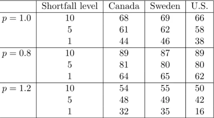
Table 5: Critical ages of clients in Canada, Sweden, and the United States based on selected levels of shortfall risk (given as percentages of the perfect hedging price) for risk indifference, risk taking, and risk aversion
Shortfall level Canada Sweden U.S.
p= 1.0 10 68 69 66 5 61 62 58 1 44 46 38 p= 0.8 10 89 87 89 5 81 80 80 1 64 65 62 p= 1.2 10 54 55 50 5 48 49 42 1 32 35 16
As an example, suppose that a risk-indifferent firm accepts a shortfall level of 5 per cent. For all three countries, the critical ages are close to 60. This implies that the premium received from a 60-year-old policyholder would guarantee the firm hedging its liability (the payoff of the shorted equity-linked contract) with the expected loss of no more than the amount equal to 5 per cent of the perfect hedging price. Recall from section 7.1 that the perfect hedging price is US$10,587.54.
A natural question arises: what are the risk implications when clients below or above the age of 60 wish to purchase the same contract? To keep the shortfall level at 5 per cent, the firm needs a particular amount of funds (as determined by (24)) to invest into a hedging strategy. Therefore, clients of all ages must pay this amount as the contract premium. Clients above 60 will be paying more than their fair share, as their survival probabilities are lower than those of a 60-year-old. However, clients below 60 will enjoy purchasing the contracts at a discount, compared with the premium they should have paid.
From Table 5, we see that the proportion of people purchasing contracts at a discount decreases with lower levels of acceptable shortfall. This is logical: the less financial risk the firm is willing to carry, the larger the proportion of people who have to pay higher premiums for the contract. Conversely, the riskier the firm (in terms of acceptable shortfall), the more discounts it can offer to its clients: the proportion of people under the critical age increases with higher shortfall levels. Moreover, this observation is reinforced in the context of the firm’s attitude to risk. Comparing the values of critical ages for p= 1, p= 0.8, and
p= 1.2, we see that a risk-taking firm offers more discounts, and a risk-averse one less, than a risk-indifferent company for the same level of shortfall. This result holds for for all the countries in consideration.
Finally, note that the critical ages for clients from the United States are almost always lower, and from Sweden they are almost always higher, than the ages of clients from Canada for a given shortfall level. This, again, is the result of the specific mortality trends in the three countries: to keep the shortfall risk at a particular acceptable level, insurance firms can attract older clients in Sweden than in the United States, since these (older) Swedish clients have the same survival probabilities as their younger counterparts in the United States. Canada falls somewhere in the middle but closer to Sweden, just as in the example from the previous section.
10. Future Direction
For future studies, there are several interesting directions worth exploring. First, a natural extension of the current setting is to consider other types of insurance products and their variations. In particular, one could study term insurance agreements (in which the payoff is paid upon the death of the insured client before the maturity of the contract), and also contracts with extra benefits or provisions, such as reversionary or terminal bonuses, paid at the maturity of the contract or upon the death of the insured client. This latter type of contract incorporates elements of both life and term insurance, with payoff to be received at the maturity of the agreement, but with a bonus paid at or before maturity, at a random time.
Second, one could study efficient hedging in the context of mortality modelling, as was done in Melnikov and Romaniuk (2006) with quantile hedging. More specifically, the insurance firm could improve its risk management strategies by utilizing appropriate mortality models to price the mortality risks inherent in equity-linked insurance products. Models that treat mortality as a stochastic process (such as those proposed in Biffis 2005; Luciano and Vigna 2005; Dahl 2004; Lee and Carter 1992) are good alternatives to consider to the traditional life tables or models with deterministic mortality (for example, the classical actuarial models of Gompertz or Makeham).
Another possibility is to study the application of efficient hedging to credit-risk derivatives, which are contracts whose payoffs are conditioned on the firm’s default or bankruptcy. Therefore, unlike in our setting, where the financial payoff is independent of the insurance event in the life of the policyholder, the study of credit-risk derivatives would require an analysis of optimal hedging in a setting where the payof