Clustering Dependencies over Relational Tables

(1)

Clustering Dependencies over

Relational Tables

by

Yuchen Gao

A thesis

presented to the University Of Waterloo

in fulfilment of the

thesis requirement for the degree of

Master of Mathematics

In

Computer Science

Waterloo, Ontario, Canada, 2015

c

(2)

Author’s Declaration

I hereby declare that I am the sole author of this thesis. This is a true copy of the thesis, including any required final revisions, as accepted by my examiners.

I understand that my thesis may be made electronically available to the public.

(3)

Abstract

Integrity constraints have proven to be valuable in the database field. Not only can they help schema design (functional dependencies, FDs [1][2]), they can also be used in query optimization (ordering dependencies, ODs [4][5][8][9]), or data cleaning (conditional functional dependencies, CFDs [12] and denial constraints, DCs [14]). In this thesis, however, we will introduce a new type of integrity constraint, called aclustering dependency (CD). Similar to ordering dependencies which rely on the database operation ORDER BY, clustering dependencies focus on studying the operation GROUP BY. Furthermore, we claim that clustering dependencies are use-ful not only in query optimization as most integrity constraints do, but also useful in data visualization, data analysis and MapReduce.

In this thesis, we first introduce some examples of clustering dependen-cies in a real-life dataset. We then formally define clustering dependendependen-cies and elaborate on our motivation. We will also look into the reasoning system for clustering dependencies including the implication problem, consistency problem and influence rules for clustering dependencies. After that, we will propose two algorithms for clustering dependencies, first a checking algo-rithm that is able to check if a given dependency is valid in a table within O(N ∗M) time, with N being the number of rows andM being the size of potentially aggregated attributes, a.k.a, the size of the right-hand-side at-tributes. Secondly, we propose a mining algorithm that is able to discover all potential clustering dependencies occurring in a table. Finally, we will use both synthetic and real-life data to test the performance of our mining algorithm.

(4)

Acknowledgements

First and foremost, I would like to give my most sincere gratitude to my supervisor, Prof. Grant Weddell. He granted me the idea of this thesis in the first place, and provided a lot of advice and guidance. I would also like to thank Prof. David Toman, he took part in our discussion a lot and provide us with some fantastic ideas. I wouldn’t have accomplished this Master’s thesis without their help. I really learned a lot from them and have improved a lot. Besides, I would like to thank the thesis committee members: Prof. Tamer Ozsu and Prof. Richard Trefler, for their kindness in reading my thesis and giving me advice.

In addition, I would like to thank my friends, Xu Chu and Jian Li, for discussing problem in thesis with me and sharing insights on different research projects all the time.

Last but no least, I would like to thank my parents, who always loved and supported me all these years.

(5)

Chapter 1

Introduction

1.1

Overview

The “group by" operations in SQL are crucial in formulating aggregate queries over intermediate results. In particular, such operations ensure inter-mediate results are ordered in ways that ensure the computation of aggregate functions can be accomplished in linear time.

In this thesis, we introduce a new class of dependencies, calledclustering dependencies (CDs), that encapsulate the necessary properties of intermedi-ate results that ensure linear scans suffice to compute aggregintermedi-ate functions.

To illustrate CDs, consider an intermediate result consisting of a set of tuples that provide bindings for the following attributes: Row ID, Order ID, Order Date, Ship Date, Ship Mode, Customer ID, Customer Name, Segment, Country, City, State, Postal Code, Region, Prod-uct ID, Category, Sub-Category, ProdProd-uct Name, Sales, Quantity, Discount and Profit. This intermediate result comes from a table that contains orders information obtained from Superstore.

The following presents examples of CDs over this set of tuples (formal definitions will be given in the next section):

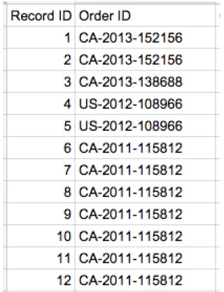
1. A CD of the form

Record ID7→ {Order ID}

will hold over the set of tuples iff any list of the same tuples that is ordered non-descending by Record ID has the property that the list is

clustered by values of Order ID, that is, has the property that no pair of tuples in the list having the same value for Order ID will have an intervening tuple in the list with a different value of Order ID.

(8)

(9)

It is intuitive that: first, if all the records are added sequentially, then Record ID would represent a timestamp for each record. Records with the same Order ID would be grouped together because items within one order won’t be separated. Second, the sameOrder IDwill not be reused in the future, otherwise the logs would be corrupted. As a result, the table is guaranteed to be grouped by Order ID. That part of the table is shown in Figure 1.1.

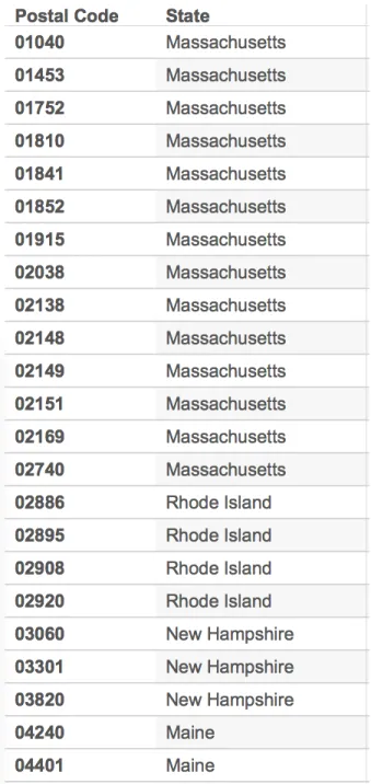
2. A CD of the form

Postal Code7→ {State}.

will hold over the set of tuples iff any list of the same tuples that is ordered non-descending byPostal Codehas the property that the list isclustered by values of State.

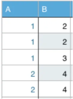
Although the fact that the table would be grouped by Statewhen it is ordered by Postal Code is not obvious, it totally makes sense. If two places have similar postal codes, then it is very likely that they are in the same state. Moreover, it is very likely that postal codes are allocated sequentially to each state. An example is shown in Figure 1.2, we can see that postal codes within range [01040, 02740] are allocated to the state Massachusetts, meaning that any postal code in this range must not belong to any state other than Massachusetts. Also, there won’t be any other postal codes from range other than [01040, 02740] that belongs to Massachusetts.

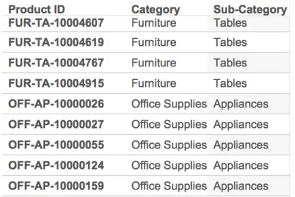
3. A CD of the form

Product ID7→ {Category, Sub-Category}.

will hold over the set of tuples iff any list of the same tuples that is ordered non-descending byProduct IDhas the property that the list isclustered by values of Categoryand Sub-Category.

If we look at the content of these attribute in the table as shown in Figure 1.3, we can see thatProduct IDis generated using first three letters of Category and Sub-Category. Considering the way this string (Product ID) is sorted: we first sort it by Category abbre-viation (like “FUR") and then by Sub-Category abbreviation (like “TA"). Thus once the table is sorted on Product ID, it would also be sorted and of course, clustered onCategoryand Sub-Category.

(10)

(11)

Figure 1.3: Dependency: Product ID 7→ {Category, Sub-Category}

From the three examples above, we can see that clustering dependencies are everywhere in our daily lives and these dependencies can show interesting facts and provide insights about the data we study.

We believe Clustering Dependencies would be useful in the following four applications:

1. Query optimization. Integrity constraints are very helpful when it comes to query optimization. Given a query, we will typically have many potential plans from which an optimizer might choose so as to provide the correct result. However, the speed of these plans can vary enormously. Integrity constraints can be applied over these plans to improve the running speed of the query.

As an integrity constraint, clustering dependencies can be used to op-timize queries that containsGROUP BY operations. If a clustering dependency is already implied in the intermediate query processing steps, then the necessity of theGROUP BY operation can be elimi-nated.

(12)

SELECT COUNT(Postcal Code) FROM TABLE T

GROUP BY State

Normally what the query processor would do is to conduct a GROUP BY operation on tableT, get the total number of postal codes for each state, and return the result. However, if the table is sorted onPostal Code already and we know clustering dependency: Postal Code 7→ {State} is valid, it would be no longer necessary for the query processor to conduct that GROUP BY operation.

2. Data visualization. We are living in a world where data is grow exponentially. But not every data owner has a comprehensive under-standing of the data they own. Data visualization, on the other hand, can help people see and understand their data by providing visual ren-dering of the them. It has become more and more important in different fields, in particular, the business intelligence (BI) field. Visualizations help people see things that were not obvious to them before. Even when data volumes are very large, patterns can be spotted quickly and easily. Visualizations convey information in a universal manner and make it simple to share ideas with others. One of the most important benefits of visualization is that it allows us access to huge amounts of data in ways that would not be otherwise possible. There are thou-sands of examples of visualizations of big data, from fun and beautiful to current and historic, to financial and political. The knowledge en-compassed in these various data sets would be nearly inaccessible to the casual, or even moderately interested viewer, if it was not visual-ized. But a good visualization gives us access to that knowledge, and does it quickly and effectively. [20]

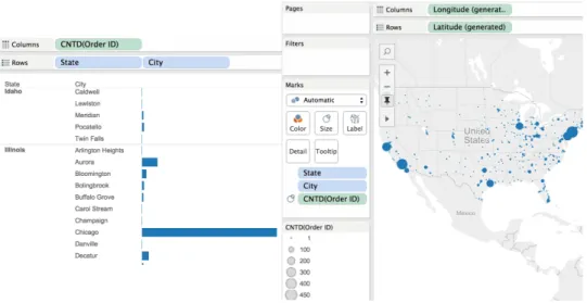
We use a commercial data visualization tool called Tableau [18] to demonstrate how data visualization works: most of the time, we can drag attributes to the “Rows" and “Column" section and the software will automatically generate a visual presentation of the data. For ex-ample, if we want to check our order table to see how many distinct orders there are for cities in different states. We will drag Stateand City to the row andSum of Order ID to the column, and get a visu-alized figure of the result, or even a graph rendered on a real map of the United States, as shown in Figure 1.4.

We can see that the way data visualization works is greatly related to the operationGROUP BY. We also found out that the speed of these

(13)

Figure 1.4: Data Visualization Example.

data visualization tools is often unsatisfactory, especially when the size of grouped by attributes is larger than 2. If we can get this operation accelerated, it would be very beneficial for data visualization.

Moreover, from the previous examples, we can observe that these de-pendencies not only improve the performance of the GROUP BY op-eration, but can also provide great insights into the data organization and the underlying semantics. This is also very helpful in data visu-alization because once we understand the semantics of the data, we can first load the data with much smarter strategies (the so-called smart-loading) and secondly, generate much more visual and beautiful rendering of the data.

3. Data analysis. Data analysis is strongly related to data visualiza-tion and is specially important and useful in the business intelligence field. The way it works is, we generate a visual representation of the data, analyze it and get the insights, and then answer questions our customers might ask about these data. Hence, once we discover the underlying semantics with clustering dependencies, we can get better much understanding of the data and thus make much better analysis and predictions.

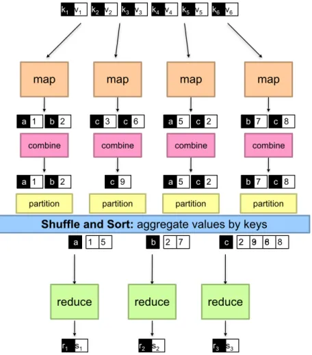
4. MapReduce. MapReduce is a programming model and an associated implementation for processing and generating large data sets with a

(14)

parallel, distributed algorithm on a cluster [21][22]. It has become ex-tremely popular in the recent decade. MapReduce works with three core phases: Map, Shuffle and Reduce. In the map phase, each worker (machine) will take a piece of input data and generate a key-value pair (k, v). These pairs would then be Shuffled to different processors according to k. Finally the reducer would process all the information associated with eachk value and produce the output. An example in shown below in Figure 1.5 [23]: the input are sent to the mappers whose output are then combined and shuffled. In the shuf-fling and sorting stage, key-value pairs with same keys are aggregated together, which is exactly a GROUP BY operation. As a result, if we could discover the underlying clustering dependency that makes the keys aggregated, then we just need to a simple sort instead of all the MapReduce operations, which is much cheaper.

In this thesis, we will explore clustering dependencies from different aspects. Our major contributions are:

1. We introduced the decision problem for clustering dependencies. We did not develop a comprehensive sound and complete reasoning system. But as long as we focus more on the algorithm and application level, we believe discovering influence rules will be able help us greatly in our preceding algorithms and experiments. In addition, we also study the relation between clustering dependencies and functional/ordering dependencies. We discovered that FDs and ODs are very useful in helping us generate more useful inference rules. We presented the inference rules we discovered as well their proof.

2. We proposed a checking algorithm for clustering dependencies to check the validity of a given CD candidate. We presented the algorithm and showed that it can run withO(N M) in time complexity in the worst case whereN is the number of rows andM is the number of attributes on the RHS of the that CD candidate.

3. We proposed a mining algorithm for clustering dependencies. We can use this mining algorithm to discover all the potential clustering de-pendencies. We also showed that our inference rules would turn out to be very helpful in the pruning process.

4. We used two types of data: synthetic data and real-life data to test the performance of our mining algorithm. Synthetic data were used

(15)

(16)

to test the performance of the mining algorithm from different as-pects. We also used real-life data from SourceForge Research Data Archive (SRDA), a Repository of FLOSS Research Data to test the performance of our mining algorithm. The SourceForge.net web site is database driven and the supporting database includes historic and status statistics on over 320,000 projects, over 850,000 developers’ ac-tivities, and over 3.4 million registered users’ activities at the project management web site [15][16][17][18]. Finally we tested with the or-ders table referred in Chapter 1 and showed the strength of our mining algorithm.

1.2

Definitions

We have seen several intuitions of clustering dependencies from the last sec-tion. They can be represented with formal clustering dependencies as follows:

• Record ID7→{Order ID}. • Postal Code7→ {State}.

• Product ID7→ {Category, Sub-Category}. Definition 1.1. Clustering Dependencies (CDs)

Let R be a relation and r be one of its instances which contains a set of tuples: t1, t2, ..., tn, letA, B1, B2, ..., Bm be the attributes in R and let ti.A

represent the value of attribute A in tuple ti, we say r satisfies Clustering Dependency A7→{B1, B2, ..., Bm}, iff the following first-order-logic (FOL) expression holds: ∀tx, ty, tz·(r(tx) ∧ r(ty) ∧ r(tz) ∧ tx.A6ty.A ∧ ty.A6tz.A ∧ Vm j=1tx.Bj =tz.Bj ⇒ Vm j=1tx.Bj =ty.Bj)

That is, for every three tuples in a relation set that is ordered by attribute A. If the first tuple has the exact same RHS values (B1, B2, ..., Bm) as the third tuple, then every tuple in between (as well as the first and third tuple) should all have the same RHS values.

Recall from the last chapter that our clustering dependencies hold when-ever the table is sorted by some attributes (the left-hand-side, LHS), then

(17)

it is guaranteed that the table is grouped by a list of attributes (the right-hand-side, RHS).

Not only can the LHS attribute Acould be any one of the attributes in R, but we also claim it could be a self-defined attribute, possibly combined with several different attributes in R. We can say that we have a attribute set {year, month, day} from R, {1990, 09, 11}, for example. We could let our LHS be a brand-new attribute named date that is composed with the valuesyear, month and day of each tuple, and sort the table by this new attribute, a.k.a,1990-09-11.

It might not be obvious why we are using an order by relationship on the LHS. Yes, we could let the LHS be a set of aggregated attributes as well just as the RHS. However, we claim that using order by on the LHS is much more useful. More importantly, according to our definition, when a set of attributes is sorted, they will be automatically aggregated as well. Moreover, with the ordering formation, we can discover a lot of more interesting depen-dencies. For instance, in our order table example in Chapter 1, the first two dependencies are about sorting by Record ID and Postal Code, respectively. If we just group either Record ID or Postal Code, then we will not be able to find out those two interesting dependencies.

Another potential concern might be that we only have one attribute on the LHS, despite the fact we can just merge multiple attributes into one and sort the table on that combined attribute. Theoretically, we could have mul-tiple attributes on the LHS, and sort by these attributes, sequentially. There are two reasons for not doing this. First, consider a clustering dependency:

Record ID7→ {Order ID}.

This dependency holds with one attributes on the LHS. However we can actually add any other attributes to the LHS as secondary key, tertiary key, etc, and it won’t change the validity of the dependency, because as long as the table is still sorted on Record ID as the prime key, it must always be grouped by Order ID.

Second, if we have multiple attributes on the LHS, it is very likely we will have to conduct more study on ordering dependencies in our framework which is not the focus of our thesis. We believe that would make our problem much more difficult to handle. We also claim that, for ordering dependen-cies, as the number of attributes grows, they would become less and less interesting and useful to us. So we will try to avoid that situation.

To make our definition more rigorous and precise, our clustering con-straint applies on set of tuples rather than list of tuples. That means, the

(18)

Figure 1.6: An violation of clustering dependency.

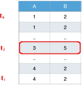
tuples are interchangeable as long as their LHS attribute is of the same value. For example, consider the following tables in Figure 1.6. Although it is a true fact the table IS sorted by attribute A and grouped by attribute B. It, however, does not satisfy the clustering constraint A 7→ {B}. Because we can exchange the first and the third row in the table, breaking the GROUP BY feature whilst still keeping the table sorted by A.

1.3

Comparison to Other Dependencies

Integrity constraints (ICs) have become more and more important nowadays when there is need to restrict the data values stored in a relational database with a series of constraints or rules to make the data accurate and consis-tent. Data integrity is the opposite of data corruption, which is a form of data loss. The overall intent of any data integrity technique is the same: ensure data is recorded exactly as intended (such as a database correctly rejecting mutually exclusive possibilities,) and upon later retrieval, ensure the data is the same as it was when it was originally recorded. In short, data integrity aims to prevent unintentional changes to information. Data integrity is not to be confused with data security, the discipline of protecting data from unauthorized parties. [19] There are a lot of integrity constraints that are already developed and well-known, like key constraints, function de-pendencies (FDs) [1][2] and conditional clustering constraints (CFDs) [12], ordering dependencies (ODs) [4][5][8][9], denial constraints (DCs) [14] and so on.

Definition 1.2. Functional Dependencies (FDs)[1][2]

A functional dependency states that the value of a specific attribute is uniquely determined by the values of a set of attributes. FD is a common

(19)

form of constraints in database system. Formally, when we are given a re-lation schema R and a relation r on R. A functional dependency X → A, whereX ⊆R andA∈R, will indicate that for any pair of tuplest, u∈r, if t[x] =u[x]for all x∈X thent[A] =u[A].

The inference axioms of functional dependencies,Armstrong’s axioms, developed by William W. Armstrong on his 1974 paper [10], can be used to infer all functional dependencies in a relational database. The axioms are soundin generating only functional dependencies in the closure of a set of functional dependencies (denoted asF+) when applied to that set (denoted asF). They are also complete in that repeated application of these rules will generate all functional dependencies in the closureF+.

Different approaches are introduced to deal with the mining problem of functional dependencies[2][3][6][7]. The mining methodologies can be divided into schema-driven and instance-driven approaches. TANE is a representa-tive for the schema-driven approach [7]. It adopts a level-wise candidate gen-eration and pruning strategy and relies on a linear algorithm for checking the validity of FDs. TANE is sensitive to the size of the schema. FASTFD is an instance-driven approach [6], which first computes agree-sets from data, then adopts a heuristic-driven depth-first search algorithm to search for covers of agree-sets. FASTFD is sensitive to the size of the instance. Both algorithms were extended in [11] for discovering CFDs [12].

Definition 1.3. Ordering Dependencies (ODs)[8][9]

An ordering dependency states that the ordering of a specific set of tu-ples are determined by another set of tutu-ples. Given a relation schemaR, an ordering dependency on a instancer on Ris represented as M N, where M and N are both sets of marked attributes,M ={Aopi1

1 , A opi₂ 2 , ..., A opim m } and N = {Bopj1 1 , B opj₂ 2 , ..., B opin n }, where A1, A2, ..., Am and B1, B2, ..., Bn are attributes fromR andopcan be=, <,6, >or_>. To better demonstrate this definition we need to define the operation u[M]v for any two tuples u and v. We say u[M]v is satisfied iff u[Ai](opi)v[Ai] is satisfied for every component{Aopi

i }inM. With that, we can say an instanceI satisfies order-ing dependencyM N iff for any two tuplesuandv,u[M]vimpliesu[N]v.

Recent papers [4][5] have come up with a variation of ordering dependen-cies, where they use lists of attributes on both LHS and RHS rather than using sets of marked attributes. In their definition, given a relation schema R, an ordering dependency is in the form ofX Y, whereXandY are both

(20)

list of attributes on a relation schemaR. We let|X|=mand|Y|=nand we will say that an ordering dependencyX Y holds if, when the relationr is ordered byx1, x2, ..., xm ∈X, it would also be ordered by y1, y2, ..., yn∈Y. In the following chapter however, we will use the first version of ordering dependency, since it would suit with our clustering dependencies better for future use.

Ordering dependencies deal with the problem of how a set of lexico-graphically ordered attributes are related to the ordering another set of lex-icographically ordered attributes. For example if the tuples are ordered by the attributes year, month, then they must also be ordered by attributes

year,quarter,monthas well. With ordering dependencies implied, when queries are processed, the query optimizer can rewrite the them to achieve better per-formance. In this case we don’t have to sort the tuples by quarter any more as long as the ordering dependency[year, quarter, month] [year, month]

is implied by the relation.

The axioms of ordering dependencies has been well-studied [4][9]. While ODs can be obtained through consultation with experts, it is an expensive process and requires expertise in the constraint language at hand as well as familiarity with the current data, thus warranting the necessity of automatic mining algorithms. However, the mining algorithm for ODs is highly non-trivial. Any list of attributes can serve as LHS and RHS of an OD. Thus the space to be explored for ODs discovery ism!×m!. Since OD focus on list of tuples rather than set of tuples and it has to deal with multiple attributes on both LHS and RHS, because an OD with multiple attributes on either side cannot be equivalently decomposed into smaller ODs. There have not been any efficient algorithm for OD mining yet. Even if there is, as the number of the attributes grows on both LHS and RHS, that dependency might become less and less interesting or helpful.

CFD discovery problem is also studied in [12], which not only is able to discover exact CFDs but also outputs approximate CFDs and dirty values for approximate CFDs, and in [13], which focuses on generating a near-optimal tableaux assuming an embedded FD is provided.

Denial constraints (DCs) significantly generalize FDs and CFDs. The complex form of DCs makes discovering them much harder. Chu et al. proposes an instance driven algorithm called FASTDC to discover DCs [14], which is quadratic w.r.t. the number of tuples due to the inherent complexity of checking if a DC is valid on a database instance. Two extensions, i.e., A-FASTDC, and C-A-FASTDC, are proposed by the same authors in order to discover DCs from dirty data, and in order to discover DCs with frequent constraints.

(21)

Chapter 2

Reasoning with Clustering

Dependencies

2.1

Overview and Preliminaries

In this chapter, we consider the decision problem and inference system w.r.t our clustering dependencies. The decision problem, which contains two sub-problems, the implication problem and consistency problem, is one of the basic problems in database field when it comes to integrity constraints. They can be very helpful to prune redundant dependencies and to test the valida-tion of new dependencies and thus without doubt could greatly benefit our clustering dependency mining process.

In the following sections, we first show that the complexity of clustering dependency decision problem is at least co-NP-complete. Then we will in-troduce and prove the inference rules we have discovered, some of which are developed with the help of functional dependencies and ordering dependen-cies.

2.2

Decision Problem

In database theory, the decision problem is one of the most classical problems to study. There are two basic decision problems in clustering dependencies for us to study. The implication problem and the consistency problem, both defined below:

Definition 2.1. The implication problem for clustering dependencies is the question whether a specific clustering dependencyd0 be implied by a

(22)

fi-nite set of dependenciesD which may contain clustering dependencies (CDs), ordering dependencies (ODs), and functional dependencies (FDs).

Definition 2.2. The consistency problem for clustering dependencies is the question whether a non-trivial model exist, given a finite set of depen-dencies D which may contain clustering dependencies (CDs), ordering de-pendencies (ODs), and functional dede-pendencies (FDs).

We need to clarify that the consistency problem is the dual of implication problem. We will say that a set of dependenciesD is inconsistent if and only if D implies a dependency of the form:

∀t·[r(t)⇒C]

whereC is any unsatisfiable constraint [24].

So we will just study the implication problem instead. As mentioned be-fore, the set of dependenciesD could contain clustering dependencies (FDs), ordering dependencies (ODs) or functional dependencies (FDs). Recall the FOL definitions for each of them. In the following content, for all the FOL formulas, we will user to represent an instance of any relational table. We use ti to denote the tuples in the table and capitalized letters to denote attributes within the table.

Clustering Dependency: A7→ {B1, B2, ..., Bm} ∀t1, t2, t3· (r(t1) ∧ r(t2) ∧ r(t3)∧ t1.A6t2.A ∧ t2.A6t3.A ∧ Vm j=1t1.Bj =t3.Bj ⇒ Vm j=1t1.Bj =t2.Bj ) Ordering Dependency: {Aop1 1 , A op2 2 , ..., A opn n } {Bop}, where opi∈ {=, <,6, >,>} ∀t1, t2· (r(t1)∧r(t2)∧ Vnj=1t1.Aj opj t2.Aj ⇒

(23)

t1.B op t2.B ) Functional Dependency: {A1, A2, ..., An} →B ∀t1, t2· (r(t1)∧r(t2)∧ Vn_j₌₁t1.Aj =t2.Aj ⇒ t1.B=t2.B )

Here we can see that FDs are special cases of ODs, hence in the following content, we will only consider ODs and CDs instead.

A study about constraint-generation dependencies [24] suggests that the implication problem for these dependencies can be linearly reduced to the validity of a universally quantified formula. The way to do this is:

First, we eliminate the quantification over tuples, which is refer as sym-metrization in [24].

Take the simplest case of a functional dependency,A →B for example, whose logic can be written as:

∀tx, ty·( r(tx)∧r(ty)∧ tx.A=ty.A ⇒ tx.B=ty.B )

According to [24], this dependency over r = {tx, ty} is equivalent to the constraint formula:

cf2(d) : [tx.A=ty.A⇒tx.B=ty.B]∧[ty.A=tx.A⇒ty.B =tx.B]

[tx.A=tx.A⇒tx.B=tx.B]∧[ty.A=ty.A⇒ty.B =ty.B] We can apply similar symmetrization process onto ordering dependencies and clustering dependencies as well. Such that the implication problem can be written as:

(∀tx1)...(∀tx3)[cf2(OD1)∧...∧cf2(ODn)∧

cf3(CD1)∧...∧cf3(CDm)⇒cf3(CD0)]

Herenandm are numbers of known ordering dependencies (ODs) and clus-tering dependencies (CDs). CD0 is the clustering dependency to be implied.

We can further replace the quantification over tuples with a quantifica-tion over elements of the domain:

(24)

(∀∗)[cf2(OD1)∧...∧cf2(ODn)∧

cf3(CD1)∧...∧cf3(CDm)⇒cf3(CD0)] (∗)

where (∀∗) quantifies all free variables in (∗). The implication problem of clustering dependencies can be linearly reduced to the validity of a univer-sally quantified formula(∗).

Now, take another look at our set of [cf2]s for ordering dependencies

and [cf3]s for clustering dependencies, all the constraints are of the form:

(tx.A op ty.A), where op∈ {=,6=, <,6}. Notice that we didn’t include > and_>since they can be replaced with <and ₆. Thus(∗) can be rewritten accordingly. First we define: ζ ::=tx.A op ty.A | ζ1∧ζ2 | ζ1 ⇒ζ2 | ¬ζ

whereop∈ {=,6=, <,6}. Then we can rewrite our implication problem as:

(∀∗)[ζ |=CD0 ]

With the constraint thatζ involves at most 3 domain variables. The paper [24] presented a theorem that states the following:

Proposition 2.3. The implication problem for clausal constraint-generating k-dependencies is:

1. in PTIME for dependencies with one atomic {=,6=, <,6}-constraint

2. co-NP-complete for dependencies with two or more atomic {=,6= }-constraints.

3. co-NP-complete for dependencies with two or more atomic {<,6 }-constraints.

However, none of the cases above suits our case because we have dependen-cies with two or more atomic {=,6=, <,6}-constraint. However, for the two remaining cases, they follow the fact that checking the satisfiability of a con-junction of equality and order constraints can be done in polynomial time.

(25)

These observations implies that the complexity of the implication problem for clustering dependencies is co-NP hard, which is unbearable. Consequently, there is a need to develop some inference rules to facilitate the implication and inference process, which could finally improve the performance of the mining algorithm that we will discuss in the next chapter.

2.3

Inference Rules

As claimed Chapter 1, functional dependencies are subsumed by ordering dependencies (The version within Definition 1.3). That is, for a functional dependency: {A, B} →C, we could rewrite it into{A=, B=} {C=}. How-ever, in this thesis, we are still considering them as two different dependen-cies. We claim that this has two benefits. First, a functional dependency is more straightforward. Second, functional dependencies are strongly related to clustering dependencies in a different way than ordering dependencies.

Inference rules can greatly help us to prone the search space. Accord-ing to our study, however, it turned out that inference rules for clusterAccord-ing dependencies alone is not that comprehensive. However, we have been able to discover that, with the help of functional dependencies and ordering de-pendencies, we will find some additional rules that can help address our CD mining problem.

Once again, in the rest of this section, we will use r to represent an instance of any relational table. We useti to denote the tuples in the table and capitalized letters to denote attributes within the table.

We will shown these rules below:

Theorem 2.4. (Empty cluster): For any attribute A, A7→ {}.

Proof: It is a empty clustering dependency and it holds trivially. Theorem 2.5. (Reflexivity): For any attribute A, A7→ {A}.

Proof: If the table is ordered by A, then it will be automatically clustered

by A as well.

Theorem 2.6. (Union): Given two clustering dependencies A 7→ S and

(26)

A7→S∪T will hold. Written as:

A7→S, A7→T A7→S∪T

Proof: LetS={B1, B2, ..., Bm}, T ={C1, C2, ..., Cn}.

Now that we have both A 7→S and A7→ T being valid, then by definition we will have: ∀tx, ty, tz·((tx.A6ty.A6tz.A ∧ Vm j=1tx.Bj =tz.Bj) ⇒ Vm j=1tx.Bj =ty.Bj) and ∀tx, ty, tz·((tx.A6ty.A6tz.A ∧ Vm j=1tx.Cj =tz.Cj) ⇒ Vm j=1tx.Cj =ty.Cj)

Putting them together, we got: ∀tx, ty, tz·((tx.A6ty.A6tz.A ∧ Vm j=1tx.Bj =ty.Bj ∧ Vm j=1tx.Cj =tz.Cj) ⇒ Vm j=1tx.Bj =ty.Bj ∧ Vmj=1tx.Cj =ty.Cj)

which is equivalent to the definition of clustering dependencyA7→S∪T.

Theorem 2.7. (Expansion with FD)Given a clustering dependencyA7→

{B1, B2, ..., Bm}and anfunctional dependencyS →C, whereS ⊆ {B1, B2, ..., Bm},

we can infer the dependency A7→ {B1, B2, ..., Bm, C}. We can also write it

as the form:

A7→ {B1, B2, ..., Bm}, S →C A7→ {B1, B2, ..., Bm, C}

Proof: First note that we did not specify thatm>1 andS 6=∅.

If m = 0 or m 6= 0 and S = ∅, we will get A 7→ {} and {} → C, with the former being a empty clustering dependency, and the latter being a functional dependency that says all the tuples have the same C value. If that is true, then we would knowC is clustered as well.

Form>1 and S6=∅,A7→ {B1, B2, ..., Bm} gives us:

(27)

⇒

Vm

j=1tx.Bj =ty.Bj)

Now, assumeA7→ {B1, B2, ..., Bm, C}does not hold, then by definition there

is at least one triple of tuplestx, ty, tz (wheretx, ty, tz are all in the relation r) that violates the rules, written as:

∃tx, ty, tz·( tx.A6ty.A6tz.A ∧ Vm j=1tx.Bj =tz.Bj ∧ tx.C =tz.C (∗) ∧ ¬(Vm j=1tx.Bj =ty.Bj)∨ ¬(tx.C =ty.C) )

Now consider (∗), since A 7→ {B1, B2, ..., Bm} then from the above

defi-nition the left part of (∗) will always be false since (Vm

j=1tx.Bj = ty.Bj)

will always be true. Now that (Vm

j=1tx.Bj = ty.Bj) is true, according to the functional dependency S → C, we can know that tx.C = ty.C is true as well. As a result, (∗) will be false which means clustering dependency A7→ {B1, B2, ..., Bm, C}will always hold.

Theorem 2.8. (OD implication) Clustering dependency can be inferred from a set of ordering dependencies, as introduced in Section 1.3. Primi-tively, given two ordering dependencies: {A<} {B6} and{A=} {B=}, we can get clustering dependency A7→B, written as:

{A<} {B6}, {A=} {B=} A7→ {B}

Proof: Assume A7→ {B} does not hold. Should that happen, by definition we will have at least one triple of tuples tx, ty, tz (where tx, ty, tz are all in the relation r) that violates the rules, written as:

∃tx, ty, tz·( tx.A6ty.A6tz.A ∧ tx.B=tz.B ∧ tx.B6=ty.B )

Let us divide the scenarios into four cases:

(1) tx.A =ty.A= tz.A (2) tx.A < ty.A < tz.A (3) tx.A < ty.A = tz.A and (4) tx.A=ty.A < tz.A.

(28)

Case 1: tx.A=ty.A=tz.A, according to the ordering dependency{A=} {B=},tx.B should be equal toty.B.

Case 2: tx.A < ty.A < tz.A, according to the ordering dependency{A<} {B6}, we will know that tx.B 6ty.B 6tz.B. If the violation occurs, then tx.B will be equal to tz.B, which means tx.B = ty.B = tz.B. Hence the violation would not occur.

Case 3: tx.A < ty.A=tz.A, according to the given ordering dependencies, we can gettx.B6ty.B=tz.B. If the violation occurs which indicates tx.B = tz.B, we will know that tx.B = ty.B = tz.B. Hence the violation would not occur.

Case 4: tx.A=ty.A < tz.A, according to the given ordering dependencies, we can gettx.B=ty.B6tz.B. If the violation occurs which indicates tx.B = tz.B, we will know that tx.B = ty.B = tz.B. Hence the violation would not occur.

Hence in general, the violation would not occur, meaningA7→ {B}will

always hold.

Theorem 2.7 also implies the following inference rules as special cases: {A<_} _{_B<_}_, _{_A=_} _{_B=_}

A7→ {B}

{A<} {B=}, {A=} {B=} A7→ {B}

Theorem 2.9. (Expansion with OD)Given a clustering dependencyA7→ {B1, B2, ..., Bm}and twoordering dependencies{A<} {C6},{A=}

{C=}, we can get the dependency A 7→ {B1, B2, ..., Bm, C} being true. We

can also write it as the form of:

A7→ {B1, B2, ..., Bm}, {A<} {C6}, {A=} {C=}

A7→ {B1, B2, ..., Bm, C}

Proof: Follows immediately from Theorem 2.5 and Theorem 2.7. Theorem 2.10. Given an ordering dependency{A<} 7→ {B₁<}, and a bunch of functional dependencies A → B1, A → B2, ... , A → Bm, we will have

(29)

clustering dependency asA7→ {B1, B2, ..., Bm}. As for:

{A<} 7→ {B₁<}, A→B1, A→B2, ..., A→Bm

A7→ {B1, B2, ..., Bm}

Proof: AssumeA7→ {B1, B2, ..., Bm}does not hold, then by definition there is at least one triple of tuples that violates the rules, written as:

∃tx, ty, tz·( tx.A6ty.A6tz.A ∧ Vm

j=1tx.Bj =tz.Bj ∧ ¬(Vm

j=1tx.Bj =ty.Bj)

According to functional dependency A → B1 and ordering dependency

{A<} 7→ {B₁<}, we will know that

1. WhenA is sorted, B1 will be sorted as well.

2. All the tuples with the sameA value should have the same B1 value.

Likewise, all the tuples with the sameB1 value should have the same

Avalue.

Now, for a violationt triple(tx, ty, tz), we must a haveVm

j=1tx.Bj =tz.Bj,

and thus we will know tx.B1 =tz.B1. According to (2), we can get tx.A= tz.A, furthermore,tx.A=ty.A=tz.A.

At this point, With tx.A=ty.A and all the remaining functional depen-dencies A → B2, A → B3, ..., A → Bm. We will know that (

Vm

j=1tx.Bj = ty.Bj). Should that be true, the violation would never occur. Thus the

orig-inal clustering constraint will hold.

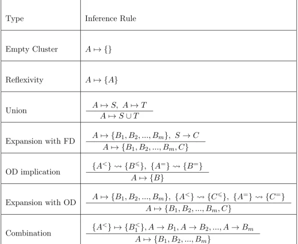
To summarize, we have discovered 7 inference rules for clustering depen-dencies, shown in Table 2.1 .

(30)

Type Inference Rule Empty Cluster A7→ {} Reflexivity A7→ {A} Union A7→S, A7→T A7→S∪T Expansion with FD A7→ {B1, B2, ..., Bm}, S→C A7→ {B1, B2, ..., Bm, C} OD implication {A <_} _{_B6_}_, _{_A=_} _{_B=_} A7→ {B} Expansion with OD A7→ {B1, B2, ..., Bm}, {A <_} _{_C6_}_, _{_A=_} _{_C=_} A7→ {B1, B2, ..., Bm, C} Combination {A <_{} 7→ {}_B< 1 }, A→B1, A→B2, ..., A→Bm A7→ {B1, B2, ..., Bm}

(31)

Chapter 3

Checking and Mining

Algorithms for Clustering

Dependencies

3.1

Clustering Dependency Validity Checking

Al-gorithm

3.1.1 Problem Definition

In this chapter, we will introduce clustering dependency validity checking algorithm.

Given a relational instancer, we use ti to represent the tuples in r and upper-case letters A, B1, B2, ..., Bk to represent attributes in r. Now given a potential clustering dependency on that instance, we want to determine whether A7→{B1, B2, ..., Bm} holds inr.

Recall the FOL representation of clustering dependencies presented in Definition 1.2: ∀tx, ty, tz·(r(tx)∧r(ty)∧r(tz)∧(tx.A6ty.A)∧(ty.A6tz.A) ∧( m ^ i=1 tx.Bi=tz.Bi)⇒( m ^ i=1 tx.Bi =ty.Bi))

a brute-force checking algorithm is quite obvious: we could enumerate every order triplet of tuple in the form of t1, t2, t3 and verify if they satisfy the

above FOL expression. If every triple satisfies the expression, we will say that this clustering dependency holds.

(32)

The correctness of this algorithm is obvious because if no violation oc-curs during the algorithm then we can assure that all the tuples satisfy the definition of CD and thus that potential CD must be valid. However, the brutal-force algorithm would take O(N3) time to enumerate all the triples and yet anotherO(m) time for to compare each attribute, making the time complexity for that would raising to O(N3m) where N is the number of tuples in instancer, andmis the number of attributes on the RHS. We can see that asN grows, the time cost of this algorithm would be huge.

In the following content, we will present an algorithm that gives us the time complexity ofO(N m), where N is the number of tuples and m is the size of RHS attributes of the clustering dependency to be verified.

3.1.2 Introduction of the Algorithm

Let us first consider the case where there is only one LHS attribute. We assume all the clustering dependencies to check are of the form:

A7→{B1, B2, ..., Bm}.

In the following content, we will denote our instance with t, and use ti to represent each tuple in the instance.

Before we introduce the algorithm. We will define another important and practical concept: “Interesting" Clustering Dependencies.

Definition 3.1. Interesting Clustering Dependency

LetA7→{B1, B2, ..., Bm} be a clustering dependency. We say this

clus-tering dependency isinterestingif either of the following two cases holds: 1. B1, B2, ..., Bm are not keys, and their values are not identical on every

row.

2. BothA andB1, B2, ..., Bm are sorted keys.

Consider the first case, the reason we add this constraint is, as the number of attributesm grows, the value combination of B1, B2, ..., Bm will be more likely to be different from each other, and eventually could become key of the table. Although by definition they are still valid clustering dependencies, they can provide us with no useful information and are not worth studying. Hence we should consider them as “uninteresting" clustering dependencies.

(33)

Also, if the RHS values of a CD are identical, that CD will hold trivially but we are not interested in that case.

The only exception for that is the second case, when the LHS is also a key and both sides are sorted. This would a special case of an ordering dependency. Hence, we could consider them “interesting" as well.

That being said, before our checking algorithm, it is necessary to check whether this CD candidate is interesting. The checking for attributes that contain identical values can be done when the table is read. The process of checking RHS for keys will be done prior to the checking algorithm for that CD candidate.

The details of the algorithm is shown below:

Preprocessing:

1. After reading in a table, found out the attributes that have only one identical value, and remove this attribute from the input.

2. For each RHS candidate, check if this RHS forms a key. If it does and the LHS is not, we will not proceed with this CD candidate.

Input for the checking algorithm:

• a table T with N rows and M columns, that contains the tuples {t1, t2, ..., tN}

• one LHS attribute, marked asA

• a set of RHS attributes, marked asB1, B2, ..., Bm, wherem6M

Main algorithm:

During the main part of the algorithm, we do a linear scan of all the tuples. Our algorithm terminates as soon as a violation is found. If the algorithm performed a scan of all tuples without finding a violation, we could consider this potential clustering dependency as valid. Our algorithm ensures that, when it reaches tupleti, then all the tuples before that, i.e., t1

to ti−1, will satisfy that clustering dependency. Consequently, when we are

atti, our job is to verify that adding this tuple will not cause any violation. To help explaining the algorithm we first introduce some variables and definitions that are used in the algorithm.

(34)

• LHS-cluster An LHS-cluster will represent a group of tuples with the same LHS value. Since for the rest of the algorithm the tuples are considered to be sorted by the LHS attribute, tuples with the same LHS value must belong to the same (and that only) LHS-cluster. Moreover, when we say “current LHS-cluster", we mean the group of tuples that has the same A value as tupleti−1 (since we will be verifyingti at that moment), and of course, these tuples must be adjacent to one another. • RHS-value A RHS-value indicates the value combination of all the RHS attributes in that clustering dependency candidate, a.k.a, B1, B2, ..., Bm. We would say that two tuples have the same RHS-value iff these two tuples have the sameBi for every i∈ {1,2, .., m}. • currentClusterMustIdentical currentClusterMustIdentical is a

boolean variable that could loosely be translated into “the tuples in the current LHS-cluster must have identical RHS-value". If this variable is true, any new tuple that comes into the current LHS-cluster with a different RHS-value is considered as a violation. This variable is used to check for violation when current tuple ti is in same LHS-cluster as ti−1.

• currentClusterIdentical currentClusterIdentical is another boolean variable that could be translated into “the tuples in the previous LHS-cluster have identical RHS-value". This variable is used to check for violation when current tuple ti is in different LHS-cluster as ti−1.

Definition 3.2. Valid Tuple/Row

Let A7→{B1, B2, ..., Bm} be a CD candidate. Our algorithm will perform a linear scan from the first tuple to the last tuple. In this process, we say a tupleti isvalid(i indicates the sequential number of that tuple) iff

1. Tuples t1, t2, ..., ti−1 are valid.

2. Within an instance composed with tuples {t1, t2, ..., ti},

A7→{B1, B2, ..., Bm} holds.

Intuitively, we say a tuple is valid if adding this tuple will not compromise the given CD.

The main logic of the algorithm is shown in Algorithm 1. We first check if RHS is a key and sort the table by the LHS attributeA. We choose to use a hash table data structure to save all the RHS-value combinations. We will use this to check whether that RHS-value has appeared in previous tuples.

(35)

The time complexity for each insert and search operation in a hash table is amortized O(1). Consequently, the total time complexity for CD checking algorithm would be O(Nm), since we need O(N) time to go through all the tuples and yet anotherO(m)time to check all the attributes on the RHS of each tuple in the worst case.

For each row, we will check its validity based on four cases. 1. Different LHS-cluster, RHS-value doesn’t exist.

The RHS-value of current tuple ti is not stored in the hash table and is not in the same LHS-cluster asti−1.

2. Same LHS-cluster, RHS-value doesn’t exist.

The RHS-value of current tuple ti is not stored in the hash table and is in the same LHS-cluster asti−1.

3. Different LHS-cluster, RHS-value exists.

The RHS-value of current tuple ti is already stored in hash table and is not in the same LHS-cluster asti−1.

4. Same LHS-cluster, RHS-value exists.

The RHS-value of current tuple ti is already stored in hash table and is in the same LHS-cluster asti−1.

If any violation occurs, the algorithm will terminate. We will discuss the outcomes for each case in the next section. Finally, if the algorithm scanned all the tuple without finding a violation, we would consider this CD candidate as a valid CD.

3.1.3 Correctness Proof

As introduced in the last section, the four situations would cover every case for each tuple. Hence every incoming tuple must fall into one of the four categories. In the algorithm, we will conduct 4 different types of condition check, one for each case, respectively, to determine if ti is violation. The outcome for each situation and the corresponding proof are shown below: Case 1: Different LHS-cluster, RHS-value doesn’t exist. In this

case,ti would always be valid. Consider the FOL for CD:

∀tx, ty, tz ·(r(tx) ∧r(ty)∧ r(tz) ∧(tx.A 6 ty.A) ∧(ty.A 6 tz.A) ∧

(Vm

(36)

Data: input table and a potential dependency A7→{B1, B2, ..., Bm}, number of rows N, number of columns M

Result: True or False(whether the above dependency holds)

if (RHS is key) return false; // uninteresting CD if (N==1) return true; // if only one tuple sortTuplesBy(table, A); // sort the tuples by LHS attribute HashInsert(r1.B1..m); // add the first tuple into hash table currentClusterIdentical = true;

currentClusterMustIdentical = false; fori←2 to ldo

if HashTableFind(ri.B1..m)==false AND ri.A6=ri−1.Athen

// CASE 1:

currentClusterIdentical=true; currentClusterMustIdentical=false; HashTableInsert(ri.B1..m);

continue ; // passes

else if HashTableFind(ri.B1..m)==false AND ri.A=ri−1.Athen

// CASE 2:

if currentClusterMustIdentical == false then currentClusterIdentical = false;

HashTableInsert(ri.B1..m);

else if HashTableFind(ri.B1..m)==true AND ri.A6=ri−1.A then

// CASE 3:

if currentClusterIdentical==true AND ri.B1..m =ri−1.B1..m then

currentClusterMustIdentical = true; currentClusterIdentical = true;

else if HashTableFind(ri.B1..m)==true AND ri.A=ri−1.A then

// CASE 4:

if currentClusterIdentical==true AND ri.B1..m =ri−1.B1..m then

currentClusterMustIdentical = true; currentClusterIdentical = true;

// If we got here, an violation occurred return false;

end

(37)

When we are atti, all the previous tuples satisfy the clustering depen-dency. That is, for all x, y, z < i, the above formula must hold. To prove adding ti will not break anything, we could replace one of the variables withti. Sinceti has different LHS-value and RHS-value from any previous tuples, we will have to prove the following:

∀tx, ty, ti ·(r(tx) ∧r(ty) ∧r(ti) ∧ (tx.A 6 ty.A) ∧ (ty.A < ti.A) ∧

(Vm

j=1tx.Bj =ti.Bj)⇒(

Vm

j=1tx.Bj =ty.Bj)).

The LHS of the this FOL expression could never be true. Thus in case

1,ti could never be a violation.

Case 2: Same LHS-cluster, RHS-value doesn’t exist. In this case, ti would be valid iff “currentClusterMustIdentical" is false.

“⇒” :

Since ti is in the same LHS-cluster with ti−1, and that it has a new

RHS-value, there must be at least two different RHS-values in the current LHS-cluster. Hence “currentClusterMustIdentical" could not be true.

“⇐” :

Sincetihas different RHS-value from all the previous tuples, it will not effect the previous tuples with different LHS-value, because its RHS-value could not equal to any one of those. Hence we only need to investigate the tuples in the current LHS-cluster. We can see that for any three tuplestx, ty in this LHS-cluster,ti would be valid if we have: ∀tx, ty, ti ·(r(tx) ∧r(ty) ∧r(ti) ∧ (tx.A 6 ty.A) ∧ (ty.A 6 ti.A) ∧

(Vm

Vm

j=1tx.Bj =ty.Bj)).

Since tx, ty and ti are all in the same LHS-cluster, they should have the same LHS value:A. Hence we can rewrite the formula as:

∀tx, ty, ti ·(r(tx) ∧r(ty) ∧r(ti) ∧ (tx.A = ty.A) ∧ (ty.A = ti.A) ∧

(Vm

Vm

j=1tx.Bj =ty.Bj)).

Now that “currentClusterMustIdentical" is false,(Vm

j=1tx.Bj =ti.Bj)

would never be true. It makes the LHS of this FOL false, and the whole FOL expression true. Thusti would be valid.

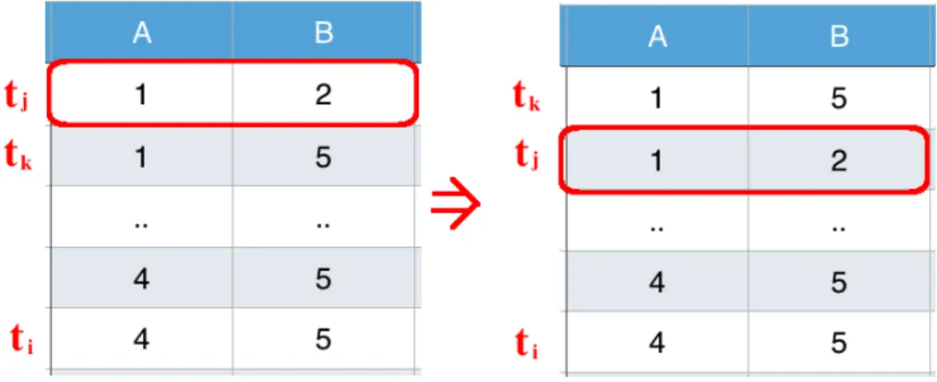
Case 3: Different LHS-cluster, RHS-value exists. In this case, ti would be valid iff (1) “currentClusterIdentical" is true and (2)ti has same RHS-value as ti−1.

(38)

Figure 3.1: Violation: tuple tj

“⇒” :

Now that we have a tuple ti whose RHS-value has occurred before, and it is in a different LHS-cluster asti−1 and all the previous tuples.

Consider any tuple that has the same RHS-value asti, saytk, then we can know the following two facts are true:

i) For any tj wherek 6j 6i, it should have the same RHS-value as tk.

ii) For any tj that are in the same LHS-cluster as tk, it should have the same RHS-value astk.

Fact i) can be easily seen. Sincetiandtkhave the same RHS-value, any tuple between them should also have the same RHS-value. Otherwise the RHS attributes would not be clustered. For example, in Figure 2.1, tj does not have the same RHS-value as tk and thus will corrupt the CD regulation.

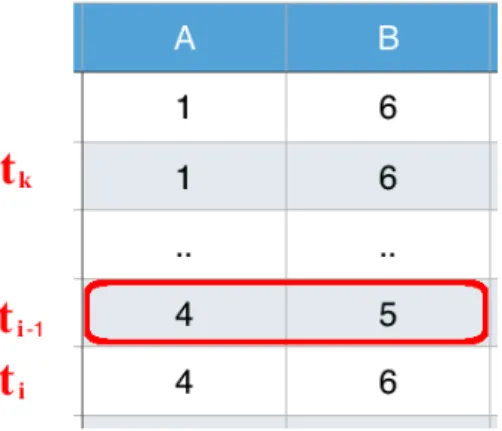
Fact ii) states that any tuple in the same LHS-cluster as tk should also have the same RHS-value as tk. This indicates that if there is any tuple in any cluster that has the same RHS-value asti, that LHS-cluster should have identical RHS-value. If we look at Figure 2.2, tk andtj are in the same LHS-cluster but have different RHS-values. Now if we swaptj andtk,tj would be sitting betweentiandtkwith different RHS-value, which is a violation of CD.

(39)

Figure 3.2: Violation: tuple tj

From the 2 facts above we can conclude that the LHS-cluster before timust have identical RHS-value, and “currentClusterIdentical" would then true. Also, since the RHS-value already exists, then there must be at least one tuple that has the same RHS-value as ti, and since those tuples must be adjacent, we can know that ti−1 must have the

same RHS-value asti.

“⇐” :

Again, consider the FOL expression:

(Vm

Vm

j=1tx.Bj =ty.Bj)).

First consider the cases where tx is in the same LHS-cluster as ti−1,

we will have: ∀tx, ty, ti ·(r(tx) ∧r(ty) ∧r(ti) ∧ (tx.A = ty.A) ∧ (ty.A < ti.A) ∧ (Vm j=1tx.Bj =ti.Bj)⇒( Vm j=1tx.Bj =ty.Bj)).

Since “currentClusterIdentical" is true and ti has same RHS-value as ti−1, it indicates thatti has the same RHS-value as every tuple in the previous LHS-cluster. Hence the expression holds.

On the other hand, if ti is not in the same LHS-cluster as ti−1. Since

“currentClusterIdentical" is true and ti has same RHS-value as ti−1,

we would know that all the previous LHS-cluster as well as ti share one common RHS-value. In the expression:

(Vm

Vm

(40)

For the LHS to be true,txshould have the same RHS-value asti. Also, we already know that tuples until ti−1 are all valid, which indicates

that tx and its LHS-cluster also share that common RHS-value with ti and the previous LHS-cluster. Thus the formula must be true.

Case 4: Same LHS-cluster, RHS-value exists. In this case, ti is valid iff (1) “currentClusterIdentical" is true and (2)ti has same RHS-value as ti−1.

“⇒” :

Using proof by contradiction, assume the statement is false, then either (1) or (2) would be false.

Consider (1) when the existed RHS-value belongs to a tuple in the current LHS-cluster. Let that tuple be tj. Since (1) is false, there would be at least one tuple that has different RHS-value asti, say tk. We could see that this violates the definition of clustering dependencies, because we can swap the order of the tuples, make tk sit between ti andtj and thus make a violation.

If the existed RHS-value belongs to a tuple in a LHS-cluster other than the current one, saytj. Since (1) is false, there would be at least one tuple that has different RHS-value as ti, say tk. Again, we can swap the order of the tuples and maketklay betweenti andtj, which would cause a violation of CD.

Consider (2), ti has a RHS-value different than ti−1. We could know

that there exists one tuple tk whose RHS-value equals toti, and that could not be ti−1. Hence no matter where it is, there would be no

valid CD within the table because ti−1 sits in-between ti and tk. An example is shown in Figure 3.3.

“⇐” :

Consider the FOL expression for a CD:

∀tx, ty, tz ·(r(tx) ∧r(ty)∧ r(tz) ∧(tx.A 6 ty.A) ∧(ty.A 6 tz.A) ∧

(Vm

j=1tx.Bj =tz.Bj)⇒(

Vm

j=1tx.Bj =ty.Bj)).

Assume that ty lies in the same LHS-cluster of ti, then we need to prove:

∀tx, ty, ti ·(r(tx) ∧r(ty) ∧r(ti) ∧ (tx.A 6 ty.A) ∧ (ty.A = ti.A) ∧

(Vm

(41)

Figure 3.3: A violation of CD

Since “currentClusterIdentical" is true, ty and ti must have the same RHS-value. If the LHS of the FOL expression is false, the FOL ex-pression itself would then be true. Otherwise, if the LHS of the FOL expression is true, it would indicate that tx has same RHS-value as ti. From that we can knowti, ty and ti have the same RHS-value, in which case the RHS of the FOL expression would be true.

On the other hand, if ty is not in the previous LHS-cluster of ti, for the LHS of the FOL expression to be true, tuples between tx and ti (inclusive) must share common RHS-value. In this case, tx and its corresponding LHS-cluster must also share that common RHS-value. The expression: ∀tx, ty, tz ·(r(tx) ∧r(ty)∧ r(tz) ∧(tx.A = ty.A) ∧(ty.A = tz.A) ∧ (Vm j=1tx.Bj =tz.Bj)⇒( Vm j=1tx.Bj =ty.Bj))

would hold trivially since tx, ty and tz will then share common

RHS-value.

3.2

Clustering Dependency Mining Algorithm

In this section, we will study the mining problem for clustering dependencies. Given a table or a set of dataset, we would like to know if there are any underlying interesting clustering dependencies that could let us understand our data and make better use of them.

However as the size of the table grows, and in particular, when the number of columns grows, the time cost of the mining algorithm could be a

(42)

big issue for us. Thus we will have to find ways to optimize our algorithm and prune the search space. We will talk about it in the following content.

3.2.1 Problem Definition

Given a relation instancer ∈R, whereR={R0, R1, ..., Rk}, a set of tuples, our CD mining algorithm is aiming to find out every clustering dependency within R. These dependencies will be of the form Ri → S, where S = {Rj1, Rj2, ..., Rjl}, and 16l6k+ 1.

We have two more specifications to make:

• First, to simply the problem, we will assume the LHS attribute of the mining algorithm is known beforehand in the following content. We do this because whichever attribute we use as the LHS, it will not make any difference to the algorithm.

• Second, for the LHS attributeRi, Ri ∈/ S, simply because Ri → {Ri} is trivial.

3.2.2 Algorithm Introduction

As claimed before, our problem is to find all the possible clustering depen-dencies in the form ofR0 →S within the S lattice, suppose S={A,B,C,D},

then our lattice will look like this in Figure 3.4:

As claimed before, we will consider that the LHS attribute is already known to the algorithm. We will let it beR.

Definition 3.3. ANode in the Latticedoes not mean the set of attributes represented in the lattice cell, it refers to the corresponding clustering de-pendency whose RHS equals the set of attributes in that cell.

Definition 3.4. Validity of Node

The validityof a node indicates whether the clustering dependency repre-sented by that node is valid.

As an intuition, consider one of the inference rules: the union rule: A7→ {B1, B2, ..., Bm}, A7→C

A7→ {B1, B2, ..., Bm, C}

(43)

Figure 3.4: An example of the complete lattice with S={A,B,C,D}.

• The first thing is that if both A 7→ {B1, B2, ..., Bm} and A 7→ C are true, we will know thatA7→ {B1, B2, ..., Bm, C}is true as well.

• Another way to look at this is, ifA7→ {B1, B2, ..., Bm, C} is false, and one of the premises, say,A7→ {B1, B2, ..., Bm}is true, then the other

premise must be false.

With that being said, once we acquire the validity of some nodes in the lattice, we will be able to discover all of the clustering dependencies in the lattice. The mining process can be done in two ways: a top-down approach and a bottom-up approach. Of course we could apply these two methods at the same time in our algorithm.

In an ideal world, with all the inference rules we know, we would be able to discover all of the clustering dependencies. But that is hardly the case most of the time. We are very likely to be stuck at some node where there is no more inference rules to help us go forward. Should this happen, we will need to use the checking algorithm we proposed in the last chapter to verify the clustering dependencies whose validity cannot be deduced solely from inference rules.

The way we use checking algorithm within mining algorithm is, we will first explore CDs with inference rules, until at some point no more depen-dencies can be inferred. At that moment, we will use the checking algorithm to check the validity of a CD, for the mining algorithm to proceed.

(44)

In the next section, we will see in detail how inference rules can be used to mine clustering dependencies.

3.2.3 Algorithm Implementation

Before we introduce the main part of the algorithm, there is another clarifi-cation we need to make.

Since we are only concerned with the mining algorithm for clustering dependencies, we will consider that all the ordering dependencies and functional dependencies are already known to the algorithm. That is, they are considered to be part of the input to the mining algorithm. We will first discover all the FDs and ODs and feed the result to the CD mining algorithm. To this end, we need to following definition:

Definition 3.5. AnInfluence Edgeis an directed edge between two nodes in the lattice. There will be an influence edge from node N1 to node N2 iff

the validity of N2 can be inferred by N1 and existing FDs/ODs.

Now we will see how we will use different types of inference rules to optimize the CD mining algorithm.

Case 1. Consider the OD implication rule:

{A<} {B6}, {A=} {B=} A7→ {B}

We can directly obtain some clustering dependencies from ordering dependencies, using Theorem 2.7:

This theorem can be easily applied in the algorithm. We only need to go through every OD and see if any CD that can be inferred from them.

Case 2. Consider the union rule in Theorem 2.5 with an example shown below:

A7→ {B}, A7→ {C, D} A7→ {B, C, D}

As introduced earlier, this inference rule can be used from both direc-tions:

(45)

Figure 3.5: Validate new clustering dependency with union rule (top-down).

For the top-down approach, assume we have already identified that bothA 7→ {B} and A 7→ {C, D} are true. Based on Theorem 2.5, we can know thatA7→ {B, C, D}must hold, as shown in Figure 3.5. In this situation, once we identified a valid clustering dependency (say, A7→ {B}), we will visted all the other unchecked nodes in the lattice that are disjoint with attributes in current RHS, and mark their union ({B, C, D}) as a valid node. We could then get a new valid CD:A7→ {B, C, D}.

As for the bottom-up approach, if we know that A 7→ {B, C, D} is false, and A7→ {B} is valid, we can know that A 7→ {C, D} must be false.

That is, once we have identified some invalid clustering dependency R0 7→ S, we can check for all the dependencies whose RHS is subset

of the RHS of current dependencyR0 7→S1. For example in our case,

the RHS ofA7→ {B}is a subset of the RHS of A7→ {B, C, D}. Once we find this, we can mark R0 7→ S2 as invalid clustering dependency

whereS2 =S−S1 (in our case, A7→ {C, D}), as shown in Figure 3.6.

Case 3. Consider the expanding rules with FD/OD with an example shown below:

R7→ {B}, B→C, D R7→ {B, C, D}

(46)

Figure 3.6: Invalidate new clustering dependency with union rule (bottom-up).

Figure 3.7: Validate new clustering dependency with FD/OD (top-down).

As claimed at the beginning of the section, we would assume that the FDs and ODs are already known. We can then account for them as base knowledge and represent them asInference Edgesin the lattice. For example, if we know a clustering dependency R 7→ {B} and a functional dependency B → C, D (which is a combination of B → C andB →D):

Based on Theorem 2.6, we will assume that clustering dependency R7→ {B, C, D}holds. In this case,B →C, Dwill act as anInference Edges that connects nodes B and BCD. It is not an edge in the original lattice, as we can see in Figure 3.7.

(47)

Figure 3.8: Invalidate new clustering dependency with FD/OD (bottom-up).

which corresponds to two different types of edges, one pointing down-wards in the lattice, as we just saw, and the other pointing updown-wards. In the first situation, we have one valid clustering dependency and one given FD/OD. We will be able to validate a new clustering dependency from them. In the algorithm, when we are at a valid node in the lattice, if there is an influence edge representing FD/OD pointing down, then we can just mark the node on the other side of the edge as valid. The other situation is as follows: we are an invalid clustering depen-dency and a related FD/OD. Based on Theorem 2.6, we can know that one of the premises must be wrong in this case, and since that given FD/OD must be correct, the clustering dependency premise should be wrong. In this case, we will draw an influence edge pointing up from the invalid node to the node representing that CD premise.

For example, if we know that R 7→ {B, C, D} is an invalid CD, and we know an FDB →CD. Then following the inference edge, we can deduce that the clustering dependencyR7→ {B} is invalid as well, as shown in Figure 3.8.

3.2.4 Main Algorithm

As introduced before, we will use both top-down and bottom-up search strategies to find out all the CDs. We will first check the validity (with our checking algorithm introduced in Section 3.1) of the second level of the lattice which contains all the single attribute and the last level which con-tains a set of all the attributes as RHS. We use these nodes because they can

(48)

Figure 3.9: An example of lattice

provide us with some good starting points for either top-down or bottom-up mining. Also checking the validity of these nodes would not cause much over-head. Once we got the validity of these nodes, we will use them as starting points and explore the whole lattice to mine CDs.

Ideally, with these starting points and the inference rules we can validate all the nodes in the lattice. However, most of cases we cannot find out the validity of every single node in the lattice with only inference rules. So whenever our algorithm cannot proceed, we need to use the check algorithm to check an unchecked node so that the mining process could proceed.

Another problem in this situation is, when we are no longer able to find CDs with inference rules, which node shall we choose to verify? In our algorithm we will use a greedy strategy and always find the node that could benefit the algorithm most. That is, the nodes with most outgoing inference edges.

(49)

Data: The input tableT, all the functional/ordering dependencies, a chosen LHS attributeR

Result: All the clustering dependencies onT with LHS beingR

Initialization;

Construct the lattice;

Use existing ordering dependencies to discover new clustering dependencies;

For each functional/ordering dependency, add an Inference Edge into the lattice graph;

Verify the nodes on the second level and last level of the lattice; // S is the set that save recently validated nodes in the

last step

newValidate = {Validity of nodes in the 2nd row and the last row}; // largestDeg is a priority queue (maximum heap) that saves

the nodes and uses degree as the keys

Generate largestDeg based on the degree of each nodes; repeat

// First, expand with the newly validated nodes whilenewValidate6=∅do

randomly choose a node p from newValidate; if p is a valid node then

S = {valid nodes found via pruning rule 1 and 3}; newValidate = newValidate + S;

end

else if p is an invalid node then

S = {invalid nodes found via pruning rule 2 and 4}; newValidate = newValidate + S;

end end

// No more inference rules can help, choose a node q = largestDeg.front();;

whileq is already verified do largestDeg.pop();

q = largestDeg.front(); end

verify node p;

mark node p as valid/invalid; apply according pruning rules onp;

newValidate = newValidate + { new validated nodes via p}; untillargestDeg =∅;

(50)

Our mining algorithm takes place on a lattice composed with a set of attributes except for the selected LHS attribute. The goal is to find out the validity of every node in the lattice and record them. An example with the attribute set being{A, B, C, D}is shown in Figure 3.9. We can see from the figure that at this stage of the algorithm we have found out the validity of 7 nodes.

To better demonstrate our algorithm, we will introduce the following concepts:

Definition 3.6. AnInference Graphcontains all the unverified nodes in the lattice and the relations between them. It is created when the algorithm starts.

Definition 3.7. Vertices of Inference GraphEvery node in the lattice is splitted into two counterparts. One indicates the node being valid (de-noted with(T rue)), the other indicates the node being invalid (denoted with

(T rue)). Both nodes will be placed into the inference graph asvertices. Definition 3.8. AKnowledge Poolof the algorithm contains the following three items:

1. All the FDs passed as inputs to the algorithm. 2. All the ODs passed as inputs to the algorithm. 3. Every verified nodes in the lattice and their status.

Definition 3.9. Edges of Inference Graph: Given two nodesN1andN2

in inference graph, there will be an edge pointing fromN1 to N2 iff we can

inferN2 fromN1 and the information in knowledge pool.

The main part of the algorithm in shown in Algorithm 2. The steps are: 1. We will use our CD checking algorithm to check the second and last level of the lattice. We will then add the validity of these nodes into our knowledge pool. For exam