Date of publication xxxx 00, 0000, date of current version xxxx 00, 0000. Digital Object Identifier 10.1109/ACCESS.2017.Doi Number
Hybrid Harmony Search Algorithm with Grey
Wolf Optimizer and Modified Opposition-based
Learning
Alaa A. Alomoush2, AbdulRahman A. Alsewari1,2 (Senior Member IEEE), Hammoudeh S. Alamri2, Khalid S. Aloufi3, and Kamal Z. Zamli2
I,IBM Centre of Excellence, Universiti Malaysia Pahang, 26300 Kuantan, Pahang, Malaysia
2Faculty of Computer Systems and Software Engineering, Universiti Malaysia Pahang, 26300 Kuantan, Pahang, Malaysia 3College of Computer Science and Engineering Taibah University Saudi Arabia
Corresponding author: (e-mail: [email protected]).
This research is partially funded by UMP DSS, UMP (RDU190334), A Novel Hybrid Harmony Search Algorithm with Nomadic People Optimizer algorithm for global optimization and feature selection, and (FRGS/1/2018/ICT05/UMP/02/1) (RDU190102), A novel Hybrid Kidney-inspired algorithm for Global Optimization Enhance Kidney Algorithm for IoT Combinatorial Testing Problem.
ABSTRACT
Most metaheuristic algorithms, including harmony search (HS), suffer from parameter selection. Many variants have been developed to cope with this problem and improve algorithm performance. In this paper, a hybrid algorithm of HS with grey wolf optimizer (GWO) has been developed to solve the problem of HS parameter selection. Then, a modified version of opposition-based learning technique has been applied on the hybrid algorithm to improve the HS exploration because HS easily gets trapped into local optima. Two HS parameters were automatically updated using GWO, namely, pitch adjustment rate and bandwidth. The proposed hybrid algorithm for global optimization problems is called HS. GWO-HS was evaluated using 24 classical benchmark functions with 30 state-of-the-art benchmark functions from CEC2014. Then, GWO-HS has been compared with recent HS variants and other well-known metaheuristic algorithms. Results show that the GWO-HS is superior over the old HS variants and other well-known metaheuristics in terms of accuracy and speed process.INDEX TERMS Computational Intelligence, Grey wolf optimizer, Harmony search, Hybrid algorithm, Metaheuristic, Optimization algorithm, CEC2014.
I. INTRODUCTION
Solving the NP-hard problem using an exhaustive search is an impractical technique because of long-time consumption and complex application. A well-known solution to solve the NP-hard problem with minimal time consumption is using a heuristic technique that can find a near-optimal solution. Heuristic algorithm sacrifices optimality or completeness to obtain quickly the best result.
Meta-heuristic algorithms are higher-level heuristic algorithms that can cover a wider range of problems, with a lack of information or high computation time [1]. The main functionality of meta-heuristic algorithms is obtained by merging rules and randomness to simulate natural phenomena, such as physical annealing in a simulated annealing (SA) algorithm [2], the human intelligence in the harmony search (HS) algorithm [3], the biological evolutionary process in an evolutionary algorithm (EA) [4], and animal behavior in Tabu search [5].
The efficiency of metaheuristic algorithms depends on the utilization of explorative and exploitative ranges through the
search process [6]. The exploitative process is accomplished by utilizing the information obtained to guide the search toward its goal. The explorative process is the capability of an algorithm to examine uncovered areas quickly within considerable search sizes. Overall performance develops if the balance between these two characteristics is established [7].
Harmony search (HS) algorithm is a well-known metaheuristic algorithm, introduced by Geem et al. [3] by mimicking the musician's process in creating a new musical harmony[8, 9]. The HS algorithm is used in different fields of optimization problems, such as engineering [10, 11], water distribution [12], structural optimization [6], music ensemble [13], and university timetable [14], Software testing [15-18]. Many other applications and variants of the HS algorithm were made according to previous survey articles [19, 20].
The success of using HS in different research fields is attributed to its characteristics. The main advantage of HS is its capability to utilize exploration and exploitation simultaneously through the search process [14].
Most metaheuristic algorithms, including HS, suffer from parameter selection, and premature convergence. Many variants have been developed to cope with this problem and improve algorithm performance [21-26].
Generally, researchers have two ways of setting metaheuristic parameter values, namely, by using parameter tuning or by using parameter control.
A. PARAMETER TUNING
The use of parameter tuning is achieved by finding the best values for algorithm parameters before running the algorithm to fix the problem. Parameter tuning involves a number of difficulties, such as longtime consumption because of the need to cover all possibilities, which is practically impossible; another difficulty is high complexity because parameters are not independent; moreover, choosing a fixed parameter as optimal value through the search process is against the idea of EA of a dynamic and adaptive process[27].
B. PARAMETER CONTROL
The other way to modify algorithm parameter values is through the search process, which can be accomplished in three ways.
1: First method: The algorithm parameter values can be modified using a deterministic function to replace the static value of the parameters in the search process; an example of this process is the improved HS by Mahdavi et al. [21], who replaced the static values of pitch adjustment rate (PAR) and bandwidth (BW) with new functions to modify their values throughout the search process. The following equations present the dynamic BW:
𝐶 = (𝑙𝑛 (𝐵𝑊 𝑚𝑖𝑛 𝐵𝑊 𝑚𝑎𝑥
) ÷ NI) (1)
𝐵𝑊 (𝑡) = 𝐵𝑊 𝑚𝑎𝑥× 𝑒(c ×𝑡). (2)
(BWmin; BWmax) are the minimum and maximum values of BW, t is the current number of iterations. The following equation present the dynamic PAR:
PAR(t) = PARmin+
(PARmax – PARmin)
𝑁𝐼 × t. (3)
(PARmin; PARmax) are minimum and maximum values of PAR, t is the current number of iterations, NI is the total number of iterations.
2: Second method: The algorithm can use feedback from the search process to improve the search parameter values, such as updating step size (by decreasing or increasing it) on the basis of the success rate of the search process.
3: Third method: The third method uses the self-adaptive values of the algorithm parameters. The adapted parameters can change in chromosomes and mutation processes on the basis of the previous results; an
example of this approach is the self-adaptive global best HS algorithm by Pan et al. who constructed the mutated values of harmony memory consideration rate (HMCR) and PAR through the search process
.
In the current article, we present a hybrid algorithm of HS and grey wolf optimizer (GWO). GWO is a newly developed algorithm inspired by the hunting and leadership of grey wolf packs [28]. Inspired by the idea of finding the best values using optimization algorithms, GWO was used in the current paper to modify the HS parameters as a self-adaptive process. Hence, instead of tuning the PAR and BW parameters before the search start, the GWO algorithm modifies the parameter values throughout the search process.
To improve HS exploration and avoid premature convergence, a modified version of the original opposition-based learning (OBL) [29] is implemented in the hybrid algorithm. This paper mainly aims to design, implement, and evaluate a new hybrid algorithm of HS and GWO with self-adaptive parameter selection. This paper also aims to improve HS algorithm exploration using a modified version of the OBL technique.
To evaluate the effectiveness of the suggested hybrid algorithm, the hybrid algorithm has been tested using 24 classical benchmark functions with 30 state-of-the-art benchmark functions from CEC and compared them with previous HS variants as well as with well-known metaheuristic algorithms. Parametric tests, namely, Wilcoxon’s rank test and Friedman test, were used. The tests were used to provide an insight into the new hybrid algorithm in contrast to the previous variants and hybrid algorithm at α = 5% significance level. The new hybrid algorithm shows highly competitive results in all experiments. To find the best values of harmony memory size (HMS) and HMCR for the hybrid algorithm, some experiments were conducted as presented in the experimental results and analysis section.
The remaining sections of this paper are organized as follows. The original HS and its variants. Then GWO algorithm and modified OBL are investigated. The proposed algorithm is described after that. Then, a section will provide the results and discussion. Finally, a conclusion is provided, and possible future improvements are provided.
II. HS and its Variants
In this part, we will comprehensively describe HS, and different variants were created to overcome the HS variable selection and improve its performance. Some researchers utilized fuzzy logic to automatically update the HS parameters [40]. Mahdavi et al. [21], created a modified variant of HS by adding new functions to modify the HMCR and PAR values throughout the search process. Other researchers, such as Omran et al. [22], modified the search process, which he borrowed from Particle Swarm Optimization [41].
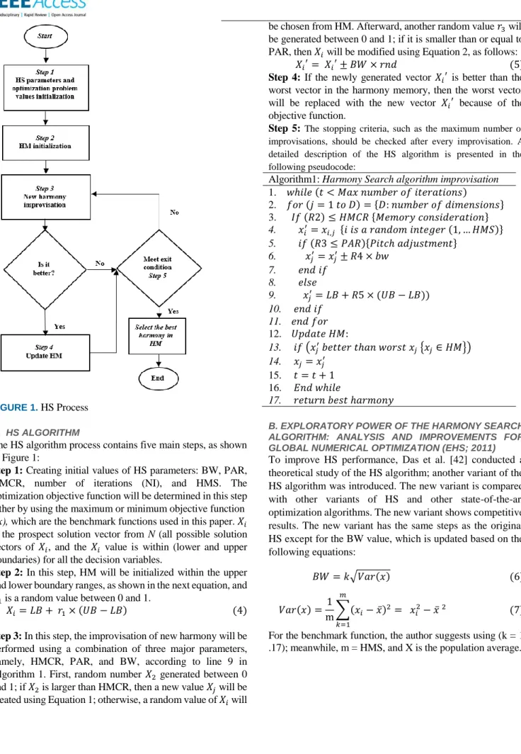
FIGURE 1.HS Process
A. HS ALGORITHM
The HS algorithm process contains five main steps, as shown in Figure 1:
Step 1: Creating initial values of HS parameters: BW, PAR, HMCR, number of iterations (NI), and HMS. The optimization objective function will be determined in this step either by using the maximum or minimum objective function
f(x), which are the benchmark functions used in this paper. 𝑋𝑖 is the prospect solution vector from N (all possible solution vectors of 𝑋𝑖, and the 𝑋𝑖 value is within (lower and upper boundaries) for all the decision variables.
Step 2: In this step, HM will be initialized within the upper and lower boundary ranges, as shown in the next equation, and
𝑋1 is a random value between 0 and 1.
𝑋𝑖= 𝐿𝐵 + 𝑟1× (𝑈𝐵 − 𝐿𝐵) (4)
Step 3: In this step, the improvisation of new harmony will be performed using a combination of three major parameters, namely, HMCR, PAR, and BW, according to line 9 in Algorithm 1. First, random number 𝑋2 generated between 0 and 1; if 𝑋2 is larger than HMCR, then a new value 𝑋𝑗 will be created using Equation 1; otherwise, a random value of 𝑋𝑖 will
be chosen from HM. Afterward, another random value 𝑟3 will be generated between 0 and 1; if it is smaller than or equal to PAR, then 𝑋𝑖 will be modified using Equation 2, as follows:
𝑋𝑖′= 𝑋𝑖′± 𝐵𝑊 × 𝑟𝑛𝑑 (5)
Step 4: If the newly generated vector 𝑋𝑖′ is better than the worst vector in the harmony memory, then the worst vector will be replaced with the new vector 𝑋𝑖′ because of the objective function.
Step 5: The stopping criteria, such as the maximum number of improvisations, should be checked after every improvisation. A detailed description of the HS algorithm is presented in the following pseudocode:
Algorithm1: Harmony Search algorithm improvisation
1. 𝑤ℎ𝑖𝑙𝑒 (𝑡 < 𝑀𝑎𝑥 𝑛𝑢𝑚𝑏𝑒𝑟 𝑜𝑓 𝑖𝑡𝑒𝑟𝑎𝑡𝑖𝑜𝑛𝑠) 2. 𝑓𝑜𝑟 (𝑗 = 1 𝑡𝑜 𝐷) = {𝐷: 𝑛𝑢𝑚𝑏𝑒𝑟 𝑜𝑓 𝑑𝑖𝑚𝑒𝑛𝑠𝑖𝑜𝑛𝑠} 3. 𝐼𝑓 (𝑅2) ≤ 𝐻𝑀𝐶𝑅 {𝑀𝑒𝑚𝑜𝑟𝑦 𝑐𝑜𝑛𝑠𝑖𝑑𝑒𝑟𝑎𝑡𝑖𝑜𝑛} 4. 𝑥𝑖′= 𝑥𝑖,𝑗 {𝑖 𝑖𝑠 𝑎 𝑟𝑎𝑛𝑑𝑜𝑚 𝑖𝑛𝑡𝑒𝑔𝑒𝑟 (1, … 𝐻𝑀𝑆)} 5. 𝑖𝑓 (𝑅3 ≤ 𝑃𝐴𝑅){𝑃𝑖𝑡𝑐ℎ 𝑎𝑑𝑗𝑢𝑠𝑡𝑚𝑒𝑛𝑡} 6. 𝑥𝑗′= 𝑥𝑗′± 𝑅4 × 𝑏𝑤 7. 𝑒𝑛𝑑 𝑖𝑓 8. 𝑒𝑙𝑠𝑒 9. 𝑥𝑗′= 𝐿𝐵 + 𝑅5 × (𝑈𝐵 − 𝐿𝐵)) 10. 𝑒𝑛𝑑 𝑖𝑓 11. 𝑒𝑛𝑑 𝑓𝑜𝑟 12. 𝑈𝑝𝑑𝑎𝑡𝑒 𝐻𝑀: 13. 𝑖𝑓 (𝑥𝑗′ 𝑏𝑒𝑡𝑡𝑒𝑟 𝑡ℎ𝑎𝑛 𝑤𝑜𝑟𝑠𝑡 𝑥𝑗 {𝑥𝑗∈ 𝐻𝑀}) 14. 𝑥𝑗= 𝑥𝑗′ 15. 𝑡 = 𝑡 + 1 16. 𝐸𝑛𝑑 𝑤ℎ𝑖𝑙𝑒 17. 𝑟𝑒𝑡𝑢𝑟𝑛 𝑏𝑒𝑠𝑡 ℎ𝑎𝑟𝑚𝑜𝑛𝑦
B. EXPLORATORY POWER OF THE HARMONY SEARCH ALGORITHM: ANALYSIS AND IMPROVEMENTS FOR GLOBAL NUMERICAL OPTIMIZATION (EHS; 2011)
To improve HS performance, Das et al. [42] conducted a theoretical study of the HS algorithm; another variant of the HS algorithm was introduced. The new variant is compared with other variants of HS and other state-of-the-art optimization algorithms. The new variant shows competitive results. The new variant has the same steps as the original HS except for the BW value, which is updated based on the following equations: 𝐵𝑊 = 𝑘√𝑉𝑎𝑟(𝑥) (6) 𝑉𝑎𝑟(𝑥) =1 m∑(𝑥𝑖− 𝑥̅) 2 𝑚 𝑘=1 = 𝑥𝑖2− 𝑥̅ 2 (7)
For the benchmark function, the author suggests using (k = 1 .17); meanwhile, m = HMS, and X is the population average.
TABLE 1
BENCHMARK FUNCTIONS (GOV: GLOBAL OPTIMUM VALUE).
Function Function Formula Type Range GOV
F1: Sphere ∑ 𝑥𝑖2 𝑛 𝑖=1 UM -100, 100 0 F2: Schwefel’s 2.22 ∑|𝑋𝑖| 𝐷 𝑖=1 + 𝛱𝑖=1𝐷 = |𝑋𝑖| UM -10, 10 0 F3: Step ∑(|𝑋𝑖+ 0.5|)2 𝐷 𝑖=1 UM -100, 100 0 F4: Rosenbrock ∑ 100 × (𝑋𝑖− 𝑋𝑖−12 )2+ (𝑥𝑖−1− 1)2 𝐷 𝑖=1 UM -30, 30 0 F5: Schwefel’s 2.26 − ∑ [𝑥𝑖𝑠𝑖𝑛 (√|𝑥𝑖|)] 𝑛 𝑖=1 UM -500, 500 −12569.5 F6: Rastrigin ∑(𝑋𝑖2− 10 𝑐𝑜𝑠(2𝜋𝑥𝑖) + 10) 𝐷 𝑖=1 M -5.12, 5.12 0 F7: Ackleys −20 𝑒𝑥𝑝 ( −0.2√1 30∑ 𝑥 2 𝐷 𝑖=1 ) − 𝑒𝑥𝑝 ( √1 30∑ 𝑐𝑜𝑠 2𝑥 2 𝐷 𝑖=1 ) + 20 + 𝑒 M -32, 32 0 F8: Griewank 1 4000∑ 𝑥 2 𝐷 𝑖=1 − 𝛱𝑖=1𝐷 𝑐𝑜𝑠 𝑥𝑖 √𝑖+ 1 M -600, 600 0 F9: Rotated hyper-ellipsoid ∑(∑ 𝑥𝑗 𝑗=𝑖 𝑗=1 )2 𝑛 𝑖=1 UM -100, 100 0 F10: Schaffer 0.5 +𝑠𝑖𝑛 2(√(𝑥 12+ 𝑥22) − 0.5 |1 + 0.001(𝑥12+ 𝑥 22)|2 M -100, 100 0 F11: Zakharov ∑ 𝑥𝑖2 𝑛 𝑖=1 + (∑ 0.5𝑖𝑥𝑖 𝑛 𝑖=1 ) 2 + (∑ 0.5𝑖𝑥𝑖 𝑛 𝑖=1 ) 4 M -5, 10 0 F12: Alpine ∑|𝑥𝑖 . 𝑠𝑖𝑛(𝑥𝑖) + 0.1𝑥𝑖| 𝑛 𝑖=1 M -10, 10 0
F13: Inverted Cosine Wave − ∑ 𝑒(−(𝑥𝑖
2+𝑥 𝑖+12 +0.5𝑥𝑖𝑥𝑖+1) 8 )𝑐𝑜𝑠 4 × √𝑥 𝑖2+ 𝑥𝑖+12 + 0.5𝑥𝑖𝑥𝑖+1 𝑛−1 𝑖=1 M -1, 1 0 F14: Dixon price (𝑥1− 1)2+ ∑ 𝑖(2𝑥𝑖2− 𝑥𝑖− 1)2 𝑛 𝑖=1 UM -10, 10 0
F15: Axis parallel hyper-ellipsoid 2.2 ∑ 𝑖 × 𝑋𝑖2 𝐷 𝑖=1 UM -5.12, 5.12 0 F16: Sum of a different power 2.8 ∑ 𝑋𝑖{1+𝑖} {𝐷} {𝑖=1} UM -1, 1 0
F17: Levy 𝑠𝑖𝑛2(𝜋𝜔 1) + ∑(𝜔𝑖− 1)2[1 + 10\𝑠𝑖𝑛2(𝜋𝜔𝑖+ 1)] 𝐷−1 𝑖=1 + (𝜔𝐷− 1)2[1 +\𝑠𝑖𝑛2(2𝜋𝜔𝐷)] M -10, 10 0 F18: Salomon’s 2.8 1 − 𝑐𝑜𝑠(2𝜋 | 𝑥 |) + 0.1| 𝑥 | , | 𝑥 | = √∑ 𝑥𝑖 2 𝑛 𝑖=1 M -100, 100 0 F19: Pathologic ∑[0.5 +] 𝑠𝑖𝑛2(√{100𝑥𝑖 2+𝑥 {𝑖+1}2 }) − 0.5 1 + 0.001 (𝑥𝑖2− 2𝑥𝑖𝑥{𝑖+1}+ 𝑥{𝑖+1}2 ) 2 𝑛−1 𝑖=1 M -100, 100 0 F20: Whitley's ∑ ∑ ((100(𝑥𝑖2− 𝑥𝑗) 2 + (1 − 𝑥𝑗) 2 )2 4000 𝑛 𝑖=1 𝑛 𝑖=1 − 𝑐𝑜𝑠 (100(𝑥𝑖2− 𝑥𝑗) 2 + (1 − 𝑥𝑗) 2 ) + 1) M -10, 10 0 F21: Schwefel's problem 2.21 𝑚𝑎𝑥𝑖{|𝑥𝑖|, 1 ≤ 𝑖 ≤ 𝑛 } UM -100, 100 0 F22: Quartic ∑ 𝑖 𝑛 𝑖=0 𝑥𝑖4+ 𝑟𝑎𝑛𝑑𝑜𝑚(0,1) UM -1.28, 1.28 0 F23: Penalized 1 𝜋 𝑛× {10 × 𝑠𝑖𝑛 2(𝜋𝑦 1) +} ∑𝑛−1𝑖=1(𝑦1− 1)2[1 + 10 𝑠𝑖𝑛2(𝜋𝑦1+ 1)] + (𝑦𝑛− 1)2+ ∑𝑛𝑖=1𝑢(𝑥𝑖, a, k, m) UM -50, 50 0 F24: Penalized 2 𝜋 𝑛× {10 × 𝑠𝑖𝑛 2(𝜋𝑦 1) +} ∑𝑛−1𝑖=1(𝑦1− 1)2[1 + 10 𝑠𝑖𝑛2(𝜋𝑦1+ 1)] + (𝑦𝑛− 1)2+ ∑𝑛𝑖=1𝑢(𝑥𝑖, a, k, m) UM -50, 50 0
C. AN IMPROVED GLOBAL-BEST HARMONY SEARCH ALGORITHM (IGHS; 2013)
El-Abd [24] developed as an improved variant of GHS [22] by focusing on the explorative range at the beginning, and then on the exploitative range at the end of a search. To accomplish this, the author used Gaussian distribution to select the random pitch adjustment, as described in the next Equation:
𝑋𝑗′= 𝐻𝑀𝑑𝑟+ 𝐺𝑎𝑢𝑠𝑠(0,1) × 𝐵𝑊 (8) Where 𝐻𝑀𝑑𝑟 is a randomly selected value from HM, and Gauss is a random number with a mean of 0 and a standard deviation of 1. For pitch adjustment, the next equation is used as follows:
𝑋𝑗′= 𝐻𝑀𝑑𝑏𝑒𝑠𝑡+ ∅ × 𝐵𝑊 (9) Where 𝐻𝑀𝑑𝑏𝑒𝑠𝑡is the best value in HM based on the objective function evaluation f(x). The value φ is a random number that is uniformly distributed within the range “-1 to 1”. PAR value is decreased within the iterations to achieve great exploitation, as described by [43]. For BW, the author borrowed its formula from the IHS [21] variant. The algorithm was compared with seven previous HS-variants using the CEC 2005 benchmark function.
D. DIFFERENTIAL-BASED HARMONY SEARCH ALGORITHM FOR THE OPTIMIZATION OF CONTINUOUS PROBLEMS (DH/BEST; 2016)
Hosein et al.[25] introduced a new HS-variant by modifying two aspects of the original HS. The first modification is applied to the initialization of HS by using a new method to initiate feasible solutions with less randomness. The second modification involves replacing pitch adjustment with the applied to the initialization of HS by using a new method to initiate feasible solutions with less randomness. The second modification involves replacing pitch adjustment with the updated version inspired by the differential evolution (DE) mutation strategy and excluding the BW parameter. The following algorithm describes the new initialization processes, which is implemented by replacing the random value with a new calculation based on HMS:
Algorithm4: DH/best Initialization (Hosein 2016) 1. 𝑓𝑜𝑟(𝑗 = 1 𝑡𝑜𝐷) {𝐷 = 𝑑𝑖𝑚𝑒𝑛𝑠𝑖𝑜𝑛𝑠} 2. 𝑓𝑜𝑟(𝑖 = 1 𝑡𝑜 𝐻𝑀𝑆) 3. 𝑡𝑒𝑚𝑝𝑖= 𝐿𝐵 + ((𝑖 − 0.5 𝐻𝑀𝑆)) × (𝑈𝐵 − 𝐿𝐵) 4. 𝑒𝑛𝑑 𝑓𝑜𝑟 5. 𝑆ℎ𝑢𝑓𝑓𝑙𝑒 𝑡ℎ𝑒 𝑡𝑒𝑚𝑝𝑜𝑟𝑎𝑟𝑦 𝑎𝑟𝑟𝑎𝑦 6. 𝑓𝑜𝑟(𝑖 = 1 𝑡𝑜 𝐻𝑀𝑆) 7. 𝐻𝑀 = 𝑡𝑒𝑚𝑝𝑖 8. 𝑒𝑛𝑑 𝑓𝑜𝑟 9.𝑒𝑛𝑑 𝑓𝑜𝑟
Where UB and LB are the upper and lower bounds of the decision variables. The new variant eliminates the requirement of setting BW, and pitches are adjusted based on the distances between the pitches in HM by using DE/best/1 mutation, as described in the following Pseudo-code:
Algorithm5: DH/best Improvisation (Hosein 2016)
1: 𝑓𝑜𝑟 (𝑖 = 1 𝑡𝑜 𝐷) 2: 𝑖𝑓 (𝑟(0~1) ≤ 𝐻𝑀𝐶𝑅) 3: 𝑋𝑖′= 𝑋𝑖𝑗 (𝑖 𝑖𝑠 𝑟𝑎𝑛𝑑𝑜𝑚 𝑖𝑛𝑡𝑒𝑔𝑒𝑟 𝑓𝑟𝑜𝑚 1. . 𝐻𝑀𝑆) 4: 𝑖𝑓( 𝑟(0~1) ≤ 𝑃𝐴𝑅) 5: 𝑋𝑖′= 𝑋𝑏𝑒𝑠𝑡+ 𝑟(0~1) × (𝑋𝑟1,𝐽− 𝑋𝑟2,𝐽 ) 6: 𝑖𝑓( 𝑋𝑗′< 𝐿𝐵 𝑜𝑟 𝑋𝑗′> 𝑈𝐵) 7: 𝑋𝑗′= 𝑟(0~1) × (𝑈𝐵 − 𝐿𝐵) + 𝐿𝐵 8: 𝑒𝑛𝑑 𝑖𝑓 9: 𝑒𝑛𝑑 𝑖𝑓 10: 𝑒𝑙𝑠𝑒 11: 𝑋𝑗′= 𝑟(0~1) × (𝑈𝐵 − 𝐿𝐵) + 𝐿𝐵 12: 𝑒𝑛𝑑 𝑖𝑓 13:𝑒𝑛𝑑 𝑓𝑜𝑟
where UB and LB are the upper and lower bounds of the decision variables, 𝑟(0– 1) is the random value between 0 and 1, 𝑋𝑏𝑒𝑠𝑡 is the best 𝑋𝑖 in HM based on the objective function, and 𝑋𝑟1,𝐽 and 𝑋𝑟2,𝐽 are two random values in the 𝑗𝑡ℎ dimension.
E. A HYBRID HARMONY SEARCH AND SIMULATED ANNEALING (HS-SA; 2018)
New hybrid HS algorithm and SA algorithm were presented by Assad et al. [26], the temperature parameter in SA has been introduced inside the HS algorithm. The new hybrid algorithm adopts a similar process to the original HS, except that it has been updated to accept the poor results of the improvisation process via the probability of the temperature parameter. The temperature starts with a high value to provide high exploration, and it then decreases at each iteration to focus on exploitation through the search process. The new hybrid algorithm provided better results in comparison with the original HS and SA.
III. GWO ALGORITHM
GWO algorithm is a new metaheuristic algorithm developed by Mirjalili et al. [28], GWO has been presented as a swarm-based algorithm that simulates the natural driving life of grey wolves[30, 31]. The GWO algorithm shows high performance in many optimization problems [32-35].
The GWO algorithm divides the population into four groups, namely alpha α, beta β, Delta δ, and Omega ω.
Firstly, random populations of wolves are created. The wolves change their location through the optimization phase on the basis of the fittest wolves, which is α. Consequently, the second and third best solutions are named β, and δ, ω will be guided through the search by those wolves. In order to attack the prey, wolves will encircle the prey as described in the following equations: 𝐷 ⃗⃗⃗ = | 𝐶⃗⃗⃗ . 𝑋⃗⃗⃗ 𝑝(𝑡) − 𝑋⃗⃗⃗ (𝑡) | (10) 𝑋 ⃗⃗⃗ (𝑡 + 1) = 𝑋⃗⃗⃗ 𝑝(𝑡) − 𝐴⃗⃗⃗ . 𝐷⃗⃗⃗ (11) 𝑋
⃗⃗⃗ 𝑝 marks the location vector of the prey, and 𝑋⃗⃗⃗ marks the location vector of the grey wolf. 𝐶⃗⃗⃗ and 𝐴⃗⃗⃗ represent the coefficient vectors, whereas t indicates the current iteration value. 𝐶⃗⃗⃗ and 𝐴⃗⃗⃗ values are calculated using the following equations:
𝐴
⃗⃗⃗ = 2 𝐴⃗⃗⃗ . 𝑟⃗⃗ 1− 𝑎⃗⃗⃗ (8)
𝐶
⃗⃗⃗ = 2. 𝑟⃗⃗ 2 (9) where ⃗⃗ 𝑟1 and 𝑟⃗⃗ 2 are random vectors in (0,1), and 𝑎⃗⃗⃗ decreased from 2 to 0 through iterations.
The α, β, and δ values will be the best solution acquired thus far. Then, all the other values (wolves) are considered as ω and will be relocated with respect to α, β, and δ. The updated value of the wolves is based on the following equations:
𝐷 ⃗⃗⃗ α= | 𝐶⃗⃗⃗ 1 . 𝑋⃗⃗⃗ α− 𝑋⃗⃗⃗ | (12) 𝐷 ⃗⃗⃗ β= | 𝐶⃗⃗⃗ 2 . 𝑋⃗⃗⃗ β− 𝑋⃗⃗⃗ | (13) 𝐷 ⃗⃗⃗ δ= | 𝐶⃗⃗⃗ 3 . 𝑋⃗⃗⃗ δ− 𝑋⃗⃗⃗ | (14)
Where 𝑋⃗⃗⃗ is the location of the current solution; 𝑋⃗⃗⃗ 𝛼, 𝑋⃗⃗⃗ 𝛽, and 𝑋⃗⃗⃗ 𝛿 are the α, β, δ locations, respectively; 𝐶⃗⃗⃗ 1, 𝐶⃗⃗⃗ 2, and 𝐶⃗⃗⃗ 3 are random vectors between (0 to 2); and 𝑋⃗⃗⃗ 𝛼, 𝑋⃗⃗⃗ 𝛽, and 𝑋⃗⃗⃗ 𝛿, represent the distance between the current solution and α, β, and δ, respectively. Afterward, the final location of the current solution is calculated using the following equations:
𝑋 ⃗⃗⃗ 1= 𝑋⃗⃗⃗ α− 𝐴⃗⃗⃗ 1 . (𝐷⃗⃗⃗⃗⃗ α) (15) 𝑋 ⃗⃗⃗ 2= 𝑋⃗⃗⃗ β− 𝐴⃗⃗⃗ 2 . (𝐷⃗⃗⃗⃗⃗ β) (16) 𝑋 ⃗⃗⃗ 3= 𝑋⃗⃗⃗ δ− 𝐴⃗⃗⃗ 3 . (𝐷⃗⃗⃗⃗⃗ δ) (17) 𝑋 ⃗⃗⃗ (𝑡 + 1) = 𝑋⃗⃗⃗ 1+ 𝑋⃗⃗⃗ 2+ 𝑋⃗⃗⃗ 3 3 (18)
Where 𝐴⃗⃗⃗ 1, 𝐴⃗⃗⃗ 2, 𝐴⃗⃗⃗ 3 are random vectors between {-2a, 2a}, where a decreased from 2 to 0, within the course of iteration (t).
The final location will be calculated using Equations (10 to 12). Finally, 𝐴⃗⃗⃗ and 𝐶⃗⃗⃗ assist the exploration and exploitation as random and adaptive vectors, respectively. The entire process is described in algorithm 2.
IV. Modified opposition-based learning technique
The original OBL introduced by Tizhoosh [29], and many variants of OBL developed after that and used by different research areas [36]. Many HS variants and hybridizations utilized the OBL and its variants in the literature [37-39].
In this article we applied a modified version of the original OBL within the HS updating process, to improve the HS exploration, as described in Algorithm 3.
Algorithm2: Grey wolf algorithm
1. Initialize grey wolf population within the boundaries
𝑥𝑖(𝑖 = 1,2, … . , 𝑛) 2. Initialize A, a and C
3. Calculate the fitness of each search agent 4. 𝑥α= 𝑏𝑒𝑠𝑡 𝑠𝑒𝑎𝑟𝑐ℎ 𝑎𝑔𝑒𝑛𝑡 5. 𝑥β= 𝑠𝑒𝑐𝑜𝑛𝑑 − 𝑏𝑒𝑠𝑡 𝑠𝑒𝑎𝑟𝑐ℎ 𝑎𝑔𝑒𝑛𝑡 6. 𝑥δ= 𝑡ℎ𝑖𝑟𝑑 − 𝑏𝑒𝑠𝑡 𝑠𝑒𝑎𝑟𝑐ℎ 𝑎𝑔𝑒𝑛𝑡 7. 𝑤ℎ𝑖𝑙𝑒 (𝑡 < 𝑀𝑎𝑥 𝑛𝑢𝑚𝑏𝑒𝑟 𝑜𝑓 𝑖𝑡𝑒𝑟𝑎𝑡𝑖𝑜𝑛𝑠)do 8. 𝑓𝑜𝑟 (𝑒𝑎𝑐ℎ 𝑠𝑒𝑎𝑟𝑐ℎ 𝑎𝑔𝑒𝑛𝑡) 9. 𝑢𝑝𝑑𝑎𝑡𝑒 𝑡ℎ𝑒 𝑐𝑢𝑟𝑟𝑒𝑛𝑡 𝑠𝑒𝑎𝑟𝑐ℎ 𝑎𝑔𝑒𝑛𝑡 𝑝𝑜𝑠𝑠𝑖𝑡𝑖𝑜𝑛 𝑏𝑦 𝑒𝑞 18 10. End for 11. Update A, a, and C
12. Calculate the fitness of all search agents 13. Update 𝑥α, 𝑥β and 𝑥δ
14. 𝑡 = 𝑡 + 1
15. 𝑟𝑒𝑡𝑢𝑟𝑛 𝑋𝑎
In algorithm 3, 𝑥{𝑑} represents the new improvisation vector, r is a random value between 0, and 1, d is the number of dimensions, and 𝑥𝑖 is the modified opposition value. Once the improvisation process of HS creates a new value 𝑥𝑗, the modified opposition will be applied on the new improvisation value 𝑥𝑗 in the update section and will replace it if it is better on the basis of the objective function f.
V. PROPOSED HYBRID ALGORITHM
A hybrid algorithm is an algorithm that merges two or more algorithms to solve a problem. The goal of this algorithm is to create a new algorithm that combines advantages from these algorithms. The main purpose of this paper is to design, implement, and evaluate a new hybrid algorithm of HS and GWO with a self-adaptive parameter selection, where the benchmark functions are the case studies to evaluate the new proposed algorithm.
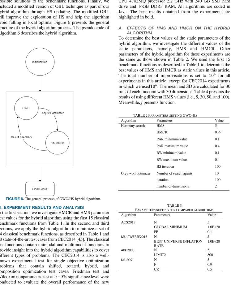
Given that the PAR and BW have a high effect on the efficiency of HS [22, 44], we utilize the GWO algorithm to find the right values of PAR and BW through the search process. We use a modified version of the original OBL technique [29] to improve improvisation results because HS suffers from bad exploration, especially if one or more of its vectors are near the local optimum. Meanwhile, we use the static values of 5 and 0.99 for HMS and HMCR, respectively. The new algorithm was tested on the benchmark function and proves the superior performance compared with the previous HS variants and other well-known metaheuristics. Figure 6 presents the general process of the hybrid algorithm, which is described as follows:
1. Hybrid algorithm parameter and population initialization:
a. Hybrid parameters will be initialized, as described in Table 2: HMCR, HMS, the minimum and maximum value of PAR and BW, number of iterations of HS (HS-NI), GWO number of iterations (GWO-NI), and the number of GWO search agents.
b. The GWO population will be initialized for PAR and BW within their upper and lower boundaries and represented as two dimensions.
c. The HS population vectors (for the benchmark functions in this paper) will be initialized using HS initialization process. These vectors will be used as HM through the whole process of the hybrid algorithm.
2. Improvisation process:
a. In the HS-improvisation process, the HM vectors will be optimized using the objective function (benchmark functions in this paper).
b. A modified OBL was used to improve the obtained result, from HS improvisation process, within the updating phase of HS, which is described in Algorithm 3. The final result is sent as a fitness function value of GWO optimization process. c. The GWO improvisation process, as described in
Algorithm 2, will be used to improvise the PAR and BW values. The fitness function (as included in line 3 in Algorithm 2) value will be the result of HS improvisation process in every GWO improvisation. 3. Results: The best results of the hybrid algorithm will be
presented in this phase.
Algorithm 6: Hybrid algorithm GWO-HS
1: Define the objective function f(x)
2: Initialize HS and GWO Parameters (HMS, HMCR, GWO-Number-of-Agents, HS-NI, GWO-NI)
3: Initialize GWO population (PARi; BWi) 4: Initialize HS population (Xi)
5: 𝑤ℎ𝑖𝑙𝑒(𝑖𝑡 < 𝐺𝑊𝑂 𝑚𝑎𝑥 𝑖𝑡𝑒𝑟𝑎𝑡𝑖𝑜𝑛)𝑑𝑜 6: 𝑤ℎ𝑖𝑙𝑒(𝑖 < 𝑠𝑒𝑎𝑟𝑐ℎ 𝑎𝑔𝑒𝑛𝑡𝑠)𝑑𝑜 7: 𝑤ℎ𝑖𝑙𝑒(𝑑 < 2)𝑑𝑜 (𝑓𝑜𝑟 𝑃𝐴𝑅 𝑎𝑛𝑑 𝐵𝑊) 8: 𝑓𝑖𝑡𝑛𝑒𝑠 = 𝐻𝑆()(HS-improvisation) 9: 𝐼𝑚𝑝𝑟𝑜𝑣𝑖𝑠𝑒 𝑛𝑒𝑤 𝑃𝐴𝑅 𝑎𝑛𝑑 𝐵𝑊(𝑢𝑠𝑖𝑛𝑔 𝐺𝑊𝑂) 10: 𝑈𝑝𝑑𝑎𝑡𝑒 𝐴𝑙𝑝ℎ𝑎, 𝐵𝑒𝑡𝑎, 𝑎𝑛𝑑 𝐷𝑒𝑙𝑡𝑎 11: 𝐼𝑚𝑝𝑟𝑜𝑣𝑖𝑠𝑒 𝑛𝑒𝑤 𝑃𝐴𝑅 𝑎𝑛𝑑 𝐵𝑊 (𝑢𝑠𝑖𝑛𝑔 𝐺𝑊𝑂 𝑖𝑚𝑝𝑟𝑜𝑣𝑖𝑠𝑎𝑡𝑖𝑜𝑛 12: 𝑝𝑟𝑜𝑐𝑒𝑠𝑠) 13: 𝑅𝑒𝑡𝑢𝑟𝑛 𝑏𝑒𝑠𝑡 ℎ𝑎𝑟𝑚𝑜𝑛𝑦
The values of PARi, BWi in Algorithm 6 are random values of
PAR and BW within their lower and upper bounds. Possible solutions for
x
i for HS initialization are the random valuesbetween the objective function boundaries.
To conclude the whole process, the GOW-initialization will be used to create PAR and BW possible values (as search agents). HS initialization will be used to initialize the benchmark functions possible solution vectors (as HM). In every iteration of GWO, the GWO-fitness function will be the result of HS optimization using the PAR and BW values from GWO-memory. HS improvisation will improvise HM values to find Algorithm3: Modified opposition
1. 𝑥{𝑑} = {𝑥1, 𝑥2, … . . 𝑥𝑑} 2. 𝑟 = 𝑟𝑎𝑛𝑑𝑜𝑚 𝑣𝑎𝑙𝑢𝑒 𝑏𝑒𝑡𝑤𝑒𝑒𝑛 (0 , 1) 3. 𝑓𝑜𝑟 (𝑖 = 1 𝑡𝑜 𝑑 )𝑑𝑜 4. 𝑋̅ = −1 × 𝑥{𝑖} × 𝑟;𝑖 5. 𝑖𝑓(𝑓(𝑥̅) < 𝑓(𝑥)) 6. x = 𝑥̅
possible solutions to the benchmark functions. Finally, we included a modified version of OBL technique as part of our hybrid algorithm through HS updating. The modified OBL will improve the exploration of HS and help the algorithm avoid falling in local optima. Figure 6 presents the general structure of the hybrid algorithm process. The pseudo code of Algorithm 6 describes the hybrid algorithm.
4.
FIGURE 6. The general process of GWO/HS hybrid algorithm. VI. EXPERIMENT RESULTS AND ANALYSIS
In the first section, we investigate HMCR and HMS parameter best values for the hybrid algorithm using the first 15 classical benchmark functions from Table 1. In the second and third sections, we apply the hybrid algorithm to minimize a set of 24 classical benchmark functions, as described in Table 1 and 30 state-of-the-art test cases from CEC2014 [45]. The classical test functions contain unimodal and multimodal functions to provide insight into the hybrid algorithm capabilities to cover different types of problems. The CEC2014 is also a well-known experimental test for single objective optimization problems that contain shifted, rotated, hybrid, and composition optimization test cases. Friedman test and Wilcoxon nonparametric test at α = 5% significance level were conducted to evaluate the overall performance of the new hybrid algorithm. All experiments are performed on Microsoft Windows 10 Education in a computer with Intel Core i7 Quad
CPU 4702MQ processor 2.2 GHz with 240 GB SSD hard drive and 16GB DDR3 RAM. All algorithms are coded in Java. The best results obtained from the experiments are highlighted in bold.
A. EFFECTS OF HMS AND HMCR ON THE HYBRID ALGORITHM
To determine the best values of the static parameters of the hybrid algorithm, we investigate the different values of the static parameters, namely, HMS and HMCR. Other parameters of the hybrid algorithm for these experiments are the same as those shown in Table 2. We used the first 15 benchmark functions as described in Table 1 to determine the best values of HMS and HMCR as static values in this article. The total number of improvisations is set to 104 for all experiments in this article, except for CEC2014 experiments in which we used106. The mean and SD are calculated for 30 runs of each function with 30 dimensions. Table 4 presents the results of using different HMS values (i.e., 5, 30, 50, and 100). Meanwhile, f presents function.
TABLE 2 PARAMETERS SETTING GWO-HS
Algorithm Parameters Value
Harmony search HMS 5
HMCR 0.99
PAR minimum value 0.1 PAR maximum value 0.4 BW minimum value 0.1 BW maximum value 0.4
HS iteration 100
Grey wolf optimizer Number of search agents 10
iteration 100
number of dimensions 2
TABLE 3
PARAMETERS SETTING FOR COMPARED ALGORITHMS
Algorithm Parameters Value
ACS2013 N 5
GLOBAL MINIMUM 1.0E+20
PP 0.1
MULTIVERSE2016 N 5
BEST UNIVERSE INFLATION RATE 1.0E+20 ABC2005 N 5 LIMIT2 800 DE1997 N 5 F 0.9 CR 0.5
TABLE 4
PARAMETERS SETTING FOR HS VARIANTS
Algorithm HMS HMCR PAR BW Other
EHS2011 5 0.99 PAR = 0.33 𝐵𝑊 = 𝑘. √𝑉𝑎𝑟(𝑥) IGHS2013 5 0.9 𝑃𝐴𝑅𝑚𝑖𝑛= 0.01 𝑃𝐴𝑅𝑚𝑎𝑥= 0.99 𝐵𝑊𝑚𝑖𝑛= 0.0001 𝐵𝑊max=0.06 DHBest2016 5 0.99 0.9 - CR=0.5 HS-SA2018 5 0.9 0.3 0.001 α =0.99 TABLE 5
EFFECTS OF HMS ON THE GWO-HS PERFORMANCE (HMCR = 0.99).
F Index HMS
5 30 50 100
F1 Mean 0.0 0.0 4.7E-147 2.1E-157
SD 0.0 0.0 4.7E-147 2.1E-157
F2 Mean 0.0 0.0 6.3E-161 2.0E-74
SD 0.0 0.0 6.3E-161 2.0E-74 F3 Mean 0.0 0.0 0.0 0.0 SD 0.0 0.0 0.0 0.0 F4 Mean 27.6 27.729 27.738 27.73 SD 27.6 27.729 27.738 27.73 F5 Mean -12528 -12500 -12494 -12454 SD 12528 12500 -2494 12454 F6 Mean 0.0 0.0 0.0 0.0 SD 0.0 0.0 0.0 0.0
F7 Mean 4.4E-16 4.4e-16 4.4e-16 4.4e-16
SD 4.4E-16 4.4e-16 4.4e-16 4.4e-16
F8 Mean 0.0 0.0 0.0 0.0 SD 0.0 0.0 0.0 0.0 F9 Mean 0.0 0.0 0.0 0.0 SD 0.0 0.0 0.0 0.0 F10 Mean 0.06 0.049 0.009 0.06 SD 0.06 0.049 0.009 0.06
F11 Mean 3.8e-14 4.0e-8 4.0e-2 1.59
SD 3.8e-14 4.0e-8 4.0e-2 1.59
F12 Mean 1.5e-53 3.2e-107 4.5e-145 0.45
SD 1.5e-53 3.2e-107 4.5 e-145 0.45
F13 Mean -26.836 -26.79 26.783 -26.87
SD 26.836 26.79 26.783 -26.87
F14 Mean 0.666 0.667 0.666 0.67
SD 0.666 0.667 0.666 0.67
F15 Mean 0.0 0.0 1.3E-241 1.3E-148
SD 0.0 0.0 1.3E-241 1.3E-148
TABLE 6
EFFECTS OF HMCR ON THE GWO-HS PERFORMANCE (HMS = 5).
F Index HMCR
0.7 0.8 0.9 0.99
F1 Mean 7.0E-24 1.4E-37 3.9E-76 0.0
SD 7.0E-24 1.4E-37 3.9E-76 0.0
F2 Mean 1.1E-1 9.6E-15 4.3E-70 0.0
SD 1.1E-1 9.6E-15 4.3E-70 0.0
F3 Mean 0.0 0.0 0.0 0.0 SD 0.0 0.0 0.0 0.0 F4 Mean 28.05 27.91 27.5 27.6 SD 28.05 27.91 27.5 27.6 F5 Mean -10081 -12091 -12552 -12528 SD -10081 -12091 -12552 12528 F6 Mean 0.0 0.0 0.0 0.0 SD 0.0 0.0 0.0 0.0
F7 Mean 3.6E-12 8.3E-13 4.4E-16 4.4E-16
SD 3.6E-12 8.3E-13 4.4E-16 4.4E-16
F8 Mean 0.0 0.0 0.0 0.0
SD 0.0 0.0 0.0 0.0
F9 Mean 6.6E-20 4.0E-34 7.1E-15 0.0
SD 6.6E-20 4.0E-34 7.1E-15 0.0
F10 Mean 8.4 0.79 0.029 0.009
SD 8.4 0.79 0.029 0.009
F11 Mean 2.59 2.60 7.7E-6 3.8e-14
SD 2.59 2.60 7.7E-6 3.8e-14 F12 Mean 0.49 0.45 0.062 1.5e-53 SD 0.49 0.45 0.062 1.5e-53 F13 Mean -26.44 -26.73 -26.87 -26.836 SD -26.44 -26.73 -26.87 26.836 F14 Mean 3.08 2.6 0.84 0.666 SD 3.08 2.6 0.84 0.666
F15 Mean 1.1E-23 1.0E-30 0.0 0.0
TABLE 7
MEAN AND SD OF THE ERRORS OF HS VARIANTS FOR (D = 30).
F Index Algorithms
EHS2011 IGHS 2013 DHBest 2016 HS-SA2018 GWO-HS
F1 Mean 2.235 e-60 14.613 0.0 10.242 0.0 SD 2.235 e-60 14.61 0.0 10.242 0.0 F2 Mean 3.484 e-35 0.179 0.0 0.851 0.0 SD 3.484 e-35 0.179 0.0 0.851 0.0 F3 Mean 0.0 20.0 0.0 11.766 0.0 SD 0.0 20.0 0.0 11.766 0.0 F4 Mean 28.712 393.048 28.767 553.709 27.766 SD 28.712 393.048 28.767 553.709 27.766 F5 Mean -10238.560 -12539.117 -12565.425 -12542.17 -12540.709 SD 10238.560 12539.117 12565.425 12542.17 12540.709 F6 Mean 0.0 3.152 0.335 1.449 0.0 SD 0.0 3.152 0.335 1.449 0.0
F7 Mean 5.417 e-15 1.841 4.440 e-16 1.610 4.440 e-16
SD 5.417 e-15 1.841 4.440 e-16 1.610 4.440 e-16
F8 Mean 8.924 e-4 1.050 0.0 1.103 0.0 SD 8.924 e-4 1.050 0.0 1.103 0.0 F9 Mean 11.881 70.978 0.0 92.409 0.0 SD 11.881 70.978 0.0 92.409 0.0 F10 Mean 0.016 0.441 0.155 0.405 0.009 SD 0.016 0.441 0.155 0.405 0.009
F11 Mean 9.206 e-5 975.251 57.17 24.633 1.002 e-5
SD 9.206 e-5 975.251 57.17 24.633 1.002 e-5
F12 Mean 5.954 e-4 0.189 0.032 0.068 1.153 e-62
SD 5.954 e-4 0.189 0.032 0.068 1.153 e-62 F13 Mean -26.530 -26.875 -26.786 -26.842 -26.753 SD 26.530 26.875 26.786 26.842 26.753 F14 Mean 0.697 4.555 10.520 7.625 0.666 SD 0.697 4.555 10.520 7.625 0.666 F15 Mean 0.032 1.45 e-5 0.033 0.10 0.0 SD 0.032 1.45 e-5 0.033 0.10 0.0
F16 Mean 3.250 e-10 4.692 e-14 1.785 e-8 1.70E-16 0.0 SD 3.250 e-10 4.692 e-14 1.785 e-8 1.70E-16 0.0
F17 Mean 1.587 0.785 2.869 0.043 0.305 SD 1.587 0.785 2.869 0.043 0.305 F18 Mean 0.103 3.506 0.0 1.867 0.0 SD 0.103 3.506 0.0 1.867 0.0 F19 Mean 1.22 2.623 0.0 1.674 0.0 SD 1.22 2.623 0.0 1.674 0.0 F20 Mean 372.07 947.823 411.16 394.573 362.217 SD 372.07 947.823 411.16 394.573 362.217 F21 Mean -2835.156 -2985.634 -2129.06 -3076.838 -2928.403 SD 2835.156 2985.634 2129.06 3076.838 2928.403 F22 Mean 4.574 8.894 6.747 8.116 2.80 SD 4.574 8.894 2 6.747 8.116 2.80 F23 Mean 0.330 2.175 1.592 0.054 0.398 SD 0.330 2.175 1.592 0.054 0.398 F24 Mean 2.086 7.155 2.938 0.448 1.976 SD 2.086 7.155 2.938 0.448 1.976
TABLE 8
MEAN AND STANDARD DEVIATION (SD) OF THE ERRORS OF HS VARIANTS FOR (D = 50).
F Index Algorithms
EHS2011 IGHS 2013 DHBest 2016 HS-SA 2018 GWO-HS
F1 Mean 3.958 e-6 382.791 0.0 524.218 0.0 SD 3.958 e-6 382.791 0.0 524.218 0.0 F2 Mean 2.08 e-5 8.310 0.0 10.119 0.0 SD 2.08 e-5 8.310 0.0 10.119 0.0 F3 Mean 0.0 280 0.0 535.9 0.0 SD 0.0 280 0.0 535.9 0.0 F4 Mean 48.869 18234 48.644 30394 47.718 SD 48.869 18234 48.644 30394 47.718 F5 Mean -12372.787 -20216 -20929 -20093 -20750 SD 12372.787 20216 20929 20093 20750 F6 Mean 2.677 41.536 1.519 45.022 0.0 SD 2.677 41.536 1.519 45.022 0.0
F7 Mean 1.678 e-4 4.366 4.440 e-16 5.711 4.440 e-16
SD 1.678 e-4 4.366 4.440 e-16 5.711 4.440 e-16
F8 Mean 0.054 2.476 0.0 5.788 0.0 SD 0.054 2.476 0.0 5.788 0.0 F9 Mean 54.862 4507.177 0.0 8509 0.0 SD 54.862 4507.177 0.0 8509 0.0 F10 Mean 0.057 0.471 0.306 0.488 0.037 SD 0.057 0.471 0.306 0.488 0.037 F11 Mean 3.165 7410.696 175.885 131.789 0.036 SD 3.165 7410.696 175.885 131.789 0.036 F12 Mean 0.103 1.08 0.051 2.329 2.528 e-68 SD 0.103 1.08 0.051 2.329 2.528 e-68 F13 Mean -42.985 -45.301 -45.144 -45.094 -45.370 SD 42.985 45.301 45.144 45.094 45.370 F14 Mean 0.724 270.194 25.759 360.223 0.666 SD 0.724 270.194 25.759 360.223 0.666 F15 Mean 0.195 17.166 0.169 23.059 0.0 SD 0.195 17.166 0.169 23.059 0.0
F16 Mean 2.50 e-9 3.774 e-12 2.799 e-7 6.07 E-13 7.591 e-19
SD 2.50 e-9 3.774 e-12 2.799 e-7 6.07 E-13 7.591 e-19
F17 Mean 3.319 7.999 1.813 1.729 2.954 SD 3.319 7.999 1.813 1.729 2.954 F18 Mean 0.129 7.635 0.0 5.176 0.0 SD 0.129 7.635 0.0 5.176 0.0 F19 Mean 3.835 5.289 0.0 4.437 0.0 SD 3.835 5.289 0.0 4.437 0.0 F20 Mean 1051.242 682667.321 1096.557 4199.406 1032.046 SD 1051.242 682667.321 1096.557 4199.406 1032.046 F21 Mean -4094.937 4539.074 -4936.221 -4894.840 -4399.1614 SD 4094.937 4539.074 4936.221 4894.840 4399.1614 F22 Mean 11.247 23.853 12.479 21.414 8.30 SD 11.247 23.8532 12.479 21.414 8.30 F23 Mean 0.527 25.025 0.652 2.710 0.579 SD 0.527 25.025 0.652 2.710 0.579 F24 Mean 4.004 173.633 3.528 22.184 3.887 SD 4.004 173.633 3.528 22.184 3.887
TABLE 9
MEAN AND STANDARD DEVIATION (SD) OF THE ERRORS FOR THE EXISTING OPTIMIZATION ALGORITHMS FOR (D = 30).
F Index Algorithms
ACS 2013 Multiverse 2016 ABC2005 DE 1997 GWO-HS
F1 Mean 3.356 e-34 0.0039 1.674 173.066 0.0 SD 3.356 e-34 0.0039 1.674 173.066 0.0 F2 Mean 5.936 e-20 0.024 0.158 0.623 0.0 SD 5.936 e-20 0.024 0.158 0.623 0.0 F3 Mean 0.0 0.666 0.0 775.266 0.0 SD 0.0 0.666 0.0 775.266 0.0 F4 Mean 33.133 28.816 2232289.712 161316.322 27.766 SD 33.133 28.816 2232289.712 161316.322 27.766 F5 Mean -12542.508 -6745.606 -11701.463 -10417.237 -12540.709 SD 12542.508 6745.606 11701.463 10417.237 12540.709 F6 Mean 0.8622 2.026 7.07 44.736 0.0 SD 0.8622 2.026 7.07 44.736 0.0 F7 Mean 0.098 0.051 2.545 6.379 4.440 e-16 SD 0.098 0.051 2.545 6.379 4.440 e-16 F8 Mean 0.001 0.009 0.348 3.338 0.0 SD 0.001 0.009 0.348 3.338 0.0 F9 Mean 8.252 e-34 0.582 0.0 2137.225 0.0 SD 8.252 e-34 0.582 0.0 2137.225 0.0 F10 Mean 0.195 0.009 0.459 0.347 0.009 SD 0.195 0.009 0.459 0.347 0.009 F11 Mean 0.871 0.001 335.010 4.624 1.002 e-5 SD 0.871 0.001 335.010 4.624 1.002 e-5
F12 Mean 1.221 e-6 0.017 0.014 0.567 1.153 e-62
SD 1.221 e-6 0.017 0.014 0.567 1.153 e-62 F13 Mean -26.864 -26.850 -26.553 -26.833 -26.753 SD 26.864 26.850 26.553 26.833 26.753 F14 Mean 0.746 0.741 3366.446 1036.294 0.666 SD 0.746 0.741 3366.446 1036.294 0.666 F15 Mean 1.186 e-36 0.001 0.230 6.354 0.0 SD 1.186 e-36 0.001 0.230 6.354 0.0
F16 Mean 2.913 e-148 9.550 e-12 1.131 e-16 1.439 e-4 0.0 SD 2.913 e-148 9.550 e-12 1.131 e-16 1.439 e-4 0.0
F17 Mean 3.349 3.349 3.349 3.349 0.305 SD 3.349 3.349 3.349 3.349 0.305 F18 Mean 0.0 0.0 0.0 0.0 0.0 SD 0.0 0.0 0.0 0.0 0.0 F19 Mean 0.0 3.250 e-10 0.0 0.0 0.0 SD 0.0 3.250 e-10 0.0 0.0 0.0 F20 Mean 413.952 413.952 413.952 413.952 362.217 SD 413.952 413.952 413.952 413.952 362.217 F21 Mean -3099.99 -2971.234 -3088.953 -3075.226 -2928.403 SD 3099.99 2971.234 3088.953 3075.226 -2928.403 F22 Mean 7.013 3.324 13.676 17.238 2.80 SD 7.013 3.324 2 13.676 17.238 2.80 F23 Mean 1.668 1.668 1.668 1.668 0.398 SD 1.668 1.668 1.668 1.668 0.398 F24 Mean 3.0 3.0 3.0 3.0 1.976 SD 3.0 3.0 3.0 3.0 1.976
TABLE 10
MEAN AND STANDARD DEVIATION (SD) OF THE ERRORS EXISTING OPTIMIZATION ALGORITHMS FOR (D = 50).
F Index Algorithms
ACS 2013 Multiverse 2016 ABC2005 DE 1997 GWO-HS
F1 Mean 5.212 e-19 0.027 1689.224 459.970 0.0 SD 5.212 e-19 0.027 1689.224 459.970 0.0 F2 Mean 5.496 e-12 0.065 6.481 1.352 0.0 SD 5.496 e-12 0.065 6.481 1.352 0.0 F3 Mean 1.4 1.633 0.3 2854.266 0.0 SD 1.4 1.633 0.3 2854.266 0.0 F4 Mean 96.360 50.836 2050687.392 2232815.458 47.718 SD 96.360 50.836 2050687.392 2232815.458 47.718 F5 Mean -20842.549 -10662.148 -17807.783 -16560.174 -20750.237 SD 20842.549 10662.148 17807.783 16560.174 20750.237 F6 Mean 4.123 5.1942 50.508 95.855 0.0 SD 4.123 5.1942 50.508 95.855 0.0 F7 Mean 0.271 0.097 9.991 9.743 4.440 e-16 SD 0.271 0.097 9.991 9.743 4.440 e-16 F8 Mean 0.004 0.057 13.013 10.318 0.0 SD 0.004 0.057 13.013 10.318 0.0 F9 Mean 3.679 e-18 18.199 26232.197 14722.357 0.0 SD 3.679 e-18 18.199 26232.197 14722.357 0.0 F10 Mean 0.384 0.042 0.497 0.477 0.037 SD 0.384 0.042 0.497 0.477 0.037 F11 Mean 24.058 0.034 667.084 144.123 0.036 SD 24.058 0.034 667.084 144.123 0.036
F12 Mean 1.573 e-4 0.114 0.619 1.804 2.528 e-68
SD 1.573 e-4 0.114 0.619 1.804 2.528 e-68 F13 Mean -45.313 -45.385 -44.409 -45.283 -45.370 SD 45.313 45.385 44.409 45.283 45.370 F14 Mean 3.910 1.022 43610.849 23618.905 0.666 SD 3.910 1.022 43610.849 23618.905 0.666 F15 Mean 7.768 e-21 0.016 88.173 41.068 0.0 SD 7.768 e-21 0.016 88.173 41.068 0.0
F16 Mean 2.123 e-124 6.993 e-12 8.463 e-5 2.128 e-4 7.591 e-19
SD 2.123 e-124 6.993 e-12 8.463 e-5 2.128 e-4 7.591 e-19
F17 Mean 5.166 5.166 5.166 5.166 2.954 SD 5.166 5.166 5.166 5.166 2.954 F18 Mean 0.0 0.0 0.0 0.0 0.0 SD 0.0 0.0 0.0 0.0 0.0 F19 Mean 0.0 0.0 0.0 0.0 0.0 SD 0.0 0.0 0.0 0.0 0.0 F20 Mean 1149.869 1149.869 1149.869 1149.869 1032.046 SD 1149.869 1149.869 1149.869 1149.869 1032.046 F21 Mean -5099.996 -4682.634 -4891.577 -5011.839 -4399.161 SD 5099.996 4682.634 4891.5774 5011.839 4399.161 F22 Mean 15.965 9.513 34.917 31.775 8.30 SD 15.965 9.513 34.917 31.775 8.30 F23 Mean 1.472 1.472 1.472 1.472 0.579 SD 1.472 1.472 1.472 1.472 0.579 F24 Mean 5.0 5.0 5.0 5.0 3.887 SD 5.0 5.0 5.0 5.0 3.887
TABLE 11
MEAN AND STANDARD DEVIATION (SD) OF THE ERRORS FOR HS VARIANTS USING THE CEC2014 (D = 30).
F Index Algorithms
EHS2011 IGHS 2013 DHBest 2016 HS-SA 2018 GWO-HS
F1 Mean 4.78 E7 2.44 E7 2.17 E7 1.64 E7 413113 SD 4.78 E7 2.44 E7 2.17 E7 1.64 E7 413113 Time 35 36 402.25 32.483 60.163 F2 Mean 1.016 E9 2799924 1.62 E8 1180792 18904 SD 1.016 E9 2799924 1.62 E8 1180792 18904 Time 20 18 219.85 17.855 20.395 F3 Mean 9247 12394 15863.40 13003 5051 SD 9247 12394 15863.40 13003 5051 Time 20 21 239.87 20.542 25.632 F4 Mean 644 533 530.31 538 439 SD 644 533 530.31 538 439 Time 21 20.45 256.36 20.926 25.033 F5 Mean 520.67 519.99 520.08 520.04 520.00 SD 520.67 519.99 520.08 520.04 520.00 Time 33.023 31.048 405.066 32.749 49.116 F6 Mean 619.58 616.68 614.96 616 620.245 SD 619.58 616.68 614.96 616 620.245 Time 3305 3499.66 39014 4057.221 6312.374 F7 Mean 708.46 700.95 708.03 700.52 700.01 SD 708.46 700.95 708.03 700.52 700.01 Time 41 40.83 485 41.882 52.229 F8 Mean 863.71 800.20 803.37 800.09 800 SD 863.71 800.20 803.37 800.09 800 Time 29 27.35 335 27.826 27.31 F9 Mean 1047.49 977.72 989.04 971.87 1037 SD 1047.49 977.72 989.04 971.87 1037 Time 36 38.59 460 39.245 37.85 F10 Mean 1995.28 1001.11 1048.71 1001.26 1001 SD 1995.28 1001.11 1048.71 1001.26 1001 Time 58 56.51 13273 60.757 63.43 F11 Mean 4479.43 3333.98 3282.25 3220.57 3793.02 SD 4479.43 3333.98 3282.25 3220.57 3793.02 Time 67 82.37 726.23 69.857 97.10 F12 Mean 1200.71 1200.16 1200.17 1200.22 1200.18 SD 1200.71 1200.16 1200.17 1200.22 1200.18 Time 690 708.27 8221 739.323 1083.54 F13 Mean 1300.64 1300.57 1300.62 1300.59 1300.55 SD 1300.64 1300.57 1300.62 1300.59 1300.55 Time 28 26.45 360.72 26.858 17.811 F14 Mean 1686.38 1660.91 1686.04 1685.41 1685.40 SD 1686.38 1660.91 1686.04 1685.41 1685.40 Time 29 26.40 370 26.07 16.18 F15 Mean 1541.48 1519.03 2321.51 1515.24 1537.52 SD 1541.48 1519.03 2321.51 1515.24 1537.52 Time 43 40.17 492 41.091 32.40 F16 Mean 1611.25 1610.12 1610.06 1610.07 1610.51 SD 1611.25 1610.12 1610.06 1610.07 1610.51 Time 42 39.22 497 41.409 31.95 F17 Mean 2699841 3011342 2894964 3716289.87 58210.62 SD 2699841 3011342 2894964 3716289.87 58210.62 Time 52 51.86 639 54.856 24.30 F18 Mean 12719 7058.42 445339 5989.24 3523.70
SD 12719 7058.42 445339 5989.24 3523.70 Time 37 34.15 437 37.037 24.30 F19 Mean 2539.23 2296.31 2534 2538.38 2539 SD 2539.23 2296.31 2534 2538.38 2539 Time 834 798.49 9895 947.406 1046 F20 Mean 14549.12 15983.76 28188 17269.85 15049.83 SD 14549.12 15983.76 28188 17269.85 15049.83 Time 37 36.81 448 30.658 49.09 F21 Mean 748419 585489 1097997 774049.91 61828 SD 748419 585489 1097997 774049.91 61828 Time 49 47.32 856 40.798 63 F22 Mean 2758 2727.08 2844 2703.86 2813 SD 2758 2727.08 2844 2703.86 2813 Time 115 114.450 1696 109.921 139.4 F23 Mean 2617 2616.48 2620.21 2616.43 2500 SD 2617 2616.48 2620.21 2616.43 2500 Time 139 139.79 1976 134.524 173.45 F24 Mean 2600 2635.87 2603 2634.43 2600 SD 2600 2635.87 2603 2634.43 2600 Time 107 111.17 1503 118.136 127.97 F25 Mean 2707 2710.26 2700.32 2709.29 2700 SD 2707 2710.26 2700.32 2709.29 2700 Time 140 142.09 1846 155.969 172.26 F26 Mean 2782 2740.74 2800.04 2766.17 2798.04 SD 2782 2740.74 2800.04 2766.17 2798.04 Time 4118 4186.60 50167 3616.477 11220.31 F27 Mean 3443 3431.52 3273.93 3401.17 2900 SD 3443 3431.52 3273.93 3401.17 2900 Time 4382 4398 45428 2723.65 5419.98 F28 Mean 4495 3925.84 4050.87 3870.42 3000 SD 4495 3925.84 4050.87 3870.42 3000 Time 299 295.40 2768 186.109 344.37 F29 Mean 16215 4177.09 2015087 4362.35 3100 SD 16215 4177.09 2015087 4362.35 3100 Time 926 825 9245 646.452 1190.62 F30 Mean 14983 11741.60.0 17050.01 11977.69 3200 SD 14983 11741.60 17050.01 11977.69 3200 Time 208 178.75 1773 126.545 369.84 TABLE 12
MEAN AND STANDARD DEVIATION (SD) OF THE ERRORS EXISTING OPTIMIZATION ALGORITHMS USING THE CEC2014 (D = 30).
F Index Algorithms
ACS 2013 MultiVerse 2016 ABC2005 DE 1997 GWO-HS
F1 Mean 68849 2463618 2.34 E7 3889379 413113 SD 68849 2463618 2.34 E7 3889379 413113 Time 273 174 113 449 60.163 F2 Mean 200 1908 993 4.76 E8 18904 SD 200 1908 993 4.76 E8 18904 Time 147 97 32 163 20.395 F3 Mean 300 374 1600.05 5684 5051 SD 300 374 1600.05 5684 5051 Time 161 95 38 197 25.632 F4 Mean 400.42 470 500.03 512 439 SD 400.42 470 500.03 512 439 Time 172 99 43 198 25.033 F5 Mean 520.01 520 520.01 520.81 520.00 SD 520.01 520 520.01 520.81 520.00
Time 228 139 89 389 49.116 F6 Mean 610.23 604.01 617.59 613 620.245 SD 610.23 604.01 617.59 613 620.245 Time 37222 16555 17323 84542 6312.374 F7 Mean 700 700.01 700.11 706.74 700.01 SD 700 700.01 700.11 706.74 700.01 Time 235 207 110 451 52.229 F8 Mean 800.91 868 800 856.48 800 SD 800.91 868 800 856.48 800 Time 162 165 12749 856.48 27.31 F9 Mean 961 971 1039.01 993 1037 SD 961 971 1039.01 993 1037 Time 231 192 85 527 37.85 F10 Mean 1000.49 2649.50 1000.08 1743 1001 SD 1000.49 2649.50 1000.08 1743 1001 Time 337 316 158 881 63.43 F11 Mean 2899.09 4168.99 3536.66 6115 3793.02 SD 2899.09 4168.99 3536.66 6115 3793.02 Time 423 360 221 1103 97.10 F12 Mean 1200.10 1200.16 1200.14 1201.50 1200.18 SD 1200.10 1200.16 1200.14 1201.50 1200.18 Time 4105 3451 3011 11534 1083.54 F13 Mean 1300.29 1300.26 1300.22 1300.40 1300.55 SD 1300.29 1300.26 1300.22 1300.40 1300.55 Time 160 167 56 215 17.811 F14 Mean 1685.39 1691 1685.39 1686.15 1685.40 SD 1685.39 1691 1685.39 1686.15 1685.40 Time 169 169 67 227 16.18 F15 Mean 1505.86 1508.67 1516.61 1612.67 1537.52 SD 1505.86 1508.67 1516.61 1612.67 1537.52 Time 243 216 116 476 32.40 F16 Mean 1609.12 1610.97 1610.11 1611.78 1610.51 SD 1609.12 1610.97 1610.11 1611.78 1610.51 Time 247 218 127 497 31.95 F17 Mean 15909.63 68155 3051313 440195.74 58210.62 SD 15909.63 68155 3051313 440195.74 58210.62 Time 348 267 203 701 24.30 F18 Mean 1970.31 3693 7320 3.09 E7 3523.70 SD 1970.31 3693 7320 3.09 E7 3523.70 Time 277 205 112 406 24.30 F19 Mean 2538.04 2547.94 2538.38 2538.97 2539 SD 2538.04 2547.94 2538.38 2538.97 2539 Time 6847 3787 3944 14593 1046 F20 Mean 2799 2227 22185.48 5931 15049.83 SD 2799 2227 22185.48 5931 15049.83 Time 246 221 118 434 49.09 F21 Mean 7125.01 34062 658713 125970 61828 SD 7125.01 34062 658713 125970 61828 Time 314 275 160 593 63 F22 Mean 2550.16 2475.32 2657.33 2486 2813 SD 2550.16 2475.32 2657.33 2486 2813 Time 721 611 503 1809 139.4 F23 Mean 2615.24 2502 2617.83 2617.13 2500 SD 2615.24 2502 2617.83 2617.13 2500 Time 999 715 662 2406 173.45 F24 Mean 2627 2600.60 2630 2646.36 2600 SD 2627 2600.60 2630 2646.36 2600
Time 781 703 500 1761 127.97 F25 Mean 2707.99 2700.08 2712 2711.38 2700 SD 2707.99 2700.08 2712 2711.38 2700 Time 1059 919 633 2227 172.26 F26 Mean 2715 2700.34 2721 2725.87 2798.04 SD 2715 2700.34 2721 2725.87 2798.04 Time 26476 21762 21399 61044 11220.31 F27 Mean 3124 2903.90 3168 3297.27 2900 SD 3124 2903.90 3168 3297.27 2900 Time 25270 21615 20556 48621 5419.98 F28 Mean 3753 3017.05 4751 3913.60 3000 SD 3753 3017.05 4751 3913.60 3000 Time 1776 1831 1339 2895 344.37 F29 Mean 3626.38 19816.49 4931 59318.770 3100 SD 3626.38 19816.49 4931 59318.770 3100 Time 6063 4775 4515 9249 1190.62 F30 Mean 5500.63 5142.61 7907 7762.58 3200 SD 5500.63 5142.61 7907 7762.58 3200 Time 1403 1232 916 1876 369.84 TABLE 13
WILCOXON SIGNED-RANK TEST RESULTS GWO-HS VS HS VARIANTS 30D.
Algorithms P-value R+ R- n/h/l/s GWO-HS vs EHS2011 0.0001 221 -52 24/21/1/2 GWO-HS vs IGHS 2013 0.00022 276 0 24/24/0/0 GWO-HS vs DHBest 2016 0.00782 217 -23 24/14/2/8 GWO-HS vs HS-SA 2018 0.00614 254 -22 24/21/3/0 TABLE 14
WILCOXON SIGNED-RANK TEST RESULTS GWO-HS VS HS VARIANTS 50D.
Algorithms P-value R+ R- n/h/l/s GWO-HS vs EHS2011 0.0001 208 -2 24/20/3/1 GWO-HS vs IGHS 2013 0.0001 251 -21 24/22/2/0 GWO-HS vs DHBest 2016 0. 02642 188 -29 24/13/3/8 GWO-HS vs HS-SA 2018 0.0002 247 -6 24/21/3/0 TABLE 15
WILCOXON SIGNED-RANK TEST RESULTS GWO-HS VS OTHER METAHEURISTICS 30D.
Algorithms P-value R+ R- n/h/l/s GWO-HS vs ACS 2013 0. 00374 225 0 24/21/0/3 GWO-HS vs MultiVerse 2016 0. 00124 228 0 24/22/0/2 GWO-HS vs ABC2005 0. 00078 213 -8 24/19/1/4 GWO-HS vs DE 1997 0. 00044 228 0 24/22/0/2 TABLE 16
WILCOXON SIGNED-RANK TEST RESULTS GWO-HS VS OTHER METAHEURISTICS 50D.
Algorithms P-value R+ R- n/h/l/s
GWO-HS vs ACS 2013 0. 00214 231 -15 24/20/2/2
GWO-HS vs MultiVerse 2016 0. 00086 240 -4 24/21/1/2
GWO-HS vs ABC2005 0. 00034 249 -8 24/20/2/2
TABLE 17
WILCOXON SIGNED-RANK TEST RESULTS GWO-HS VS HS VARIANTS CEC2014 30D.
P-value R+ R- n/h/l/s GWO-HS vs EHS2011 0.0002 414 -50 30/25/4/1 GWO-HS vs IGHS 2013 0.01778 347 -117 30/19/-11/0 GWO-HS vs DHBest 2016 0.00044 403 -62 30/24/6/0 GWO-HS vs HS-SA 2018 0.00782 359 -103 30/22/8/0 TABLE 18
WILCOXON SIGNED-RANK TEST RESULTS GWO-HS VS OTHER METAHEURISTICS CEC 2014 30D.
Algorithms P-value R+ R- n/h/l/s
GWO-HS vs ACS 2013 0. 03662 362 -103 30/22/8/0
GWO-HS vs Multiverse 2016 0. 4965 267 -195 30/17/11/2
GWO-HS vs ABC2005 0. 14706 300 -163 30/16/13/1
GWO-HS vs DE 1997 0. 00128 389 -76 30/23/7/0
FIGURE2.CONVERGENCE CURVE FOR F1
FIGURE 3. CONVERGENCE CURVE FOR F4
0 0.2 0.4 0.6 0.8 1 1 11 21 31 41 51 61 71 81 91
F1: Convergence Rate
GWO-HS Multiverse 2016 ABC 2005 ACS 2013 DE 1997 0.E+00 2.E+08 4.E+08 6.E+08 8.E+08 1.E+09 1.E+09 1.E+09 2.E+09 2.E+09 1 11 21 31 41 51 61 71 81 91F4: Convergence Rate
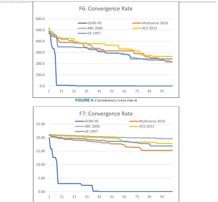
GWO-HS Multiverse 2016 ABC 2005 ACS 2013 DE 1997FIGURE4.CONVERGENCE CURVE FOR F6
FIGURE 5. CONVERGENCE CURVE FOR F7 TABLE 19
FRIEDMAN TEST RESULTS GWO-HS VS HS VARIANTS.
Algorithms Classical 30D Classical 50D CEC2014 30D
EHS2011 2.8542 2.9583 4.0833 IGHS 2013 4.1250 4.2083 2.6333 DHBest 2016 2.9792 2.1875 3.6000 HS-SA 2018 3.3750 4.1667 2.7000 GWO-HS 1.6667 1.4792 1.9833 TABLE 20
FRIEDMAN TEST RESULTS GWO-HS VS OTHER METAHEURISTICS.
Algorithms Classical 30D Classical 50D CEC2014 30D
ACS 2013 2.4792 2.5417 1.8667 Multiverse 2016 3.1458 2.8750 2.6667 ABC2005 3.6250 2.5417 3.4500 DE1997 4.1875 3.9583 4.2333 GWO-HS 1.5625 1.5000 2.7833 0.0 100.0 200.0 300.0 400.0 500.0 600.0 1 11 21 31 41 51 61 71 81 91
F6: Convergence Rate
GOW-HS Multiverse 2016 ABC 2005 ACS 2013 DE 1997 0.00 5.00 10.00 15.00 20.00 25.00 1 11 21 31 41 51 61 71 81 91F7: Convergence Rate
GOW-HS Multiverse 2016 ABC 2005 ACS 2013 DE 1997Table 4 shows that the best results for the hybrid algorithm are obtained using HMS = 5 and shows the fastest results obtained in most functions. Table 4 shows that increasing HMS does not improve the performance in most algorithms. Thus, a small HMS improves the update rate in HM for most cases. Table 5 presents the results of running the hybrid algorithm with different HMCR values (i.e., 0.7, 0.8, 0.9, and 0.99). The obtained results show that the HMCR value has a high influence on the HS performance. A large HMCR value provides improved results. The best results are obtained using HMCR = 0.99 for most benchmark functions with the fastest convergence rate. Through the experiment of HMS values, we use HMCR = 0.99 and HMS = 5 to run the HMCR value experiment.
B. EXPERIMENT 1
In this part, we will analyze the experiment of the new hybrid algorithm compared with four recent HS variants and one hybrid algorithm (i.e., EHS 2011, IGHS 2013, DH/best 2016 and HS-SA 2018). The parameter configurations for these variants are described in Table 4. The parameter values for the hybrid algorithm are the same as those listed in Table 2. First, we examine the hybrid algorithm together with four HS variants using 24 benchmark functions with 30 and 50 dimensions, as described in Table 1.
For both dimensions, as presented in Tables 7 and 8, the hybrid algorithm provides better results than the other HS variants in most cases. Second, we compare the hybrid algorithm with the recent variants of HS using 30 state-of-the-art CEC benchmark functions [45], with 30 dimensions. The results presented in Table 11 show that the new hybrid algorithm outperforms the recent variants in 20 out of the 30 test cases and provides highly competitive results. In terms of speed, the algorithm only outperforms the other variants in seven functions, but it provides high speed in all cases.
Wilcoxon’s rank test was applied to the mean results of Tables 7, 8, and 11 presented in Tables 13, 14, and 17 respectively. The p-value shows the significance of the results and performance improvement in comparison with other variants. A low p-value means high improvement. R+ presents the total ranks whenever the hybrid algorithm provides better results than the other variants, whereas R- provides the total ranks of lower results than the other variants. N is the total number of benchmark functions, l, h, and s indicate the total number of functions with higher, lower, or similar results of the hybrid algorithm compared with other variants. As presented in Tables 13, 14, and 17, the new hybrid algorithm outperforms all variants of HS with improved performance. Finally, to establish a comparative assessment, Friedman statistical test has been conducted based on the mean results of Tables 7, 8, and 11. The results presented in Table 19 confirm that the new hybrid algorithm outperforms all previous variants of HS because it provides the highest ranking. These results obtained the lowest value on the Friedman test, which shows a high ranking. The results contain classical 30D as classical benchmark functions with 30 dimensions, and classical 50D as classical benchmark functions with 50 dimensions, and finally the CEC2014 test cases with 30 dimensions.
C. EXPERIMENT 2
To investigate the capability of the hybrid algorithm, we evaluate it with other state-of-the-art metaheuristic algorithms from different families, as follows: artificial cooperative search (ACS 2013) [46], (multi-verse 2016) [47], artificial bee colony (ABC 2005)[48], and differential evolution (DE 1997) [49]. The parameter characteristics of these algorithms are shown in Table 3 as used in this experiment.
In Table 9, we compare the hybrid algorithm with other metaheuristics using classical benchmark functions as described in Table 1. These functions have 30 dimensions. The hybrid algorithm provides the best results in all test functions, except for F5 and F13. The hybrid algorithm provides the second-best results. Table 10 presents the mean, and the SD of the hybrid algorithm with other metaheuristics by using 50 dimensions for the classical benchmark functions. The hybrid algorithm outperforms other metaheuristics in all test functions, except for F5, F13, and F16; the hybrid algorithm provides the second-best result. Finally, we compare the hybrid algorithm with other metaheuristics in Table 12 using 30 state-of-the-art benchmark functions from CEC 2014. The results of mean and standard deviations and running time show that the hybrid algorithm provides the highest speed in all the 30 cases. Moreover, this algorithm outperforms all other metaheuristics in 12 cases, as presented in Table 12. Overall, according to the results shown in Tables 9 and 10, the hybrid algorithm provides a competitive result compared to other metaheuristic algorithms in terms of efficiency.
Similar to the previous section, we conducted Wilcoxon’s rank test and Friedman statistical test based on the mean results of Tables 9, 10, and 12. The Wilcoxon’s rank test results presented in Tables 15, 16, and 18 were derived from 30, 50 dimensions of classical benchmark functions, and CEC2014 test cases, respectively.
As shown in Tables 15 and 16, the hybrid algorithm provides very small p-values. Therefore, it outperforms all other metaheuristic algorithms and provides very high significant improvement. Table 18 shows the results based on CEC2014 experiment results presented in Table 12. The hybrid algorithm provides high significance results against two algorithms, namely, ACS and DE.
For the Friedman test, Table 20 presents a full overview of the classical benchmark functions with two dimensions, 30 and 50, and the CEC test cases. As seen in the classical experiments, the hybrid algorithm has the lowest value on Friedman test, which means it has the highest ranking among other metaheuristics. For the CEC2014 experiment, the hybrid algorithm has the second raking following ACS algorithm. To provide insight into the hybrid algorithm convergence rate, we run experiment using four benchmark functions. Two functions with unimodal optimum (F1, F4), and two functions with multimodal optimum (F6, F7). Figures (2 - 5) illustrate the best score obtained so far of the hybrid algorithm and other HS variants versus the iteration.
VII. CONCLUSION
This paper presents a new hybrid algorithm of the HS algorithm with the GWO algorithm called GWO-HS algorithm for the global continuous optimization problem. The