This is the author‘s version of a
work that was published in the
following source:
Patrick Jochem, Martin Schönfelder, Wolf
Fichtner, 2015
An efficient two-stage algorithm for
decentralized scheduling of micro-CHP units
In, European Journal of Operational
Research, Volume 245, Issue 3, Pages
862-874,
https://doi.org/10.1016/j.ejor.2015.04.016
Please note: Copyright is owned by the
author(s) and / or the publisher. The
commercial use of this copy is not
allowed.
An Efficient Two-stage Algorithm for Decentralized
Scheduling of Micro-CHP Units
Patrick Jochem1, Martin Schönfelder, Wolf Fichtner
Karlsruhe Institute of Technology (KIT)
Institute for Industrial Production (IIP), Chair of Energy Economics Hertzstraße 16, 76187 Karlsruhe, Germany
Abstract
In this paper we present an efficient two-stage hierarchical decomposition algorithm aiming at determining economically improved operation
schedules for residential proton exchange membrane fuel cell micro-combined heat and power (PEMFC micro-CHP) units and optimizing local charging of electric vehicles (EV) in the same household. Based on an
individual short-term load forecasting (STLF) approach (imperfect forecast) for households implemented as an adaptive network-based fuzzy inference system (ANFIS), a mixed-integer linear program (MILP) and a two-stage greedy algorithm are used for determining optimized schedules based on a rolling-window approach. The results of the case study performed for eight variants in exemplary German households reveal that with both the MILP and the algorithmic approach, significant economic savings can be achieved compared to the standard heat-led strategy. Compared to the MILP,
however, the two-stage algorithm has the additional advantage of a reduced computing time of only about 151 . Deviations from the MILP solutions are mostly smaller than 3 percent regarding the annual supply costs. Moreover, the comparison between the use of perfect and imperfect demand forecasts quantifies additional average losses due to forecasting errors of 2 percent and 3.3 percent at the maximum. Altogether, the algorithmic approach
1 Corresponding author, phone: +49-721-608 44590, fax: +49-721-608 44682, Email
address: [email protected] (Patrick Jochem)
seems to be convincing for real applications in households due to its good results, high reliability, easy implementation, and short computing times. The combination of a micro-CHP unit and an EV is highly synergetic.
Keywords: OR in Energy, PEMFC Micro-Combined Heat and Power,
Predictive Scheduling and Optimisation, Mixed-Integer Programming, Algorithmic Approach
1. Introduction
Ongoing extensive research, development, and funding activities regarding micro-combined heat and power units (micro-CHP units) are likely to enhance their distribution in small and medium-sized households. In Germany this is supported by legal measures designed to leverage the governmental target of doubling the share of CHP elec-tricity generation from about 12 percent in 2012 to 25 percent by 2020 (Federal Republic of Germany, 2012). The target will only be reached if the share of domestic micro-CHP units will grow above average com-pared to large-scale and industrial CHP (Westner & Madlener, 2011). To reach this ambitious goal, profitable micro-CHP solutions have to be developed. These are also highly efficient in terms of emission reduction. With proton exchange membrane fuel cell (PEMFC)-based micro-CHP units, the coupled generation of
electricity and heat allows for a more efficient use of primary energy due to their comparably high power to heat ratio (ρ). A PEMFC micro-CHP
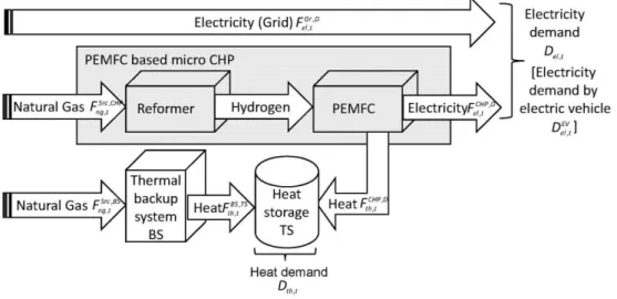
includes a reformer for generating hydrogen and a PEMFC for generating electricity and heat (cf. Fig. 2). While PEMFC systems reach values of ρ 0.6, other technologies like mostly applied gas engines (ρ 0.4) or Stirling en-gines (ρ 0.3) only reach lower values (Pehnt & Colijn, 2006; Thomas, 2011). However, especially the promising and efficient PEMFC sys-tems suffer from a limited operational flexibility (Hawkes, Brett, & Brandon, 2009) leading to economic disadvantages and, hence, to the necessity of special methods to address the challenge of reaching economically optimized operation.
1.1. Problem Setting
The key advantages of domestic micro-CHP mentioned above are only valid, if two important aspects are fulfilled:
1. The unit is operated to such an extent only that all thermal energy produced can be used in the local building either directly or with the help of a thermal buffer storage and
2. the electricity generated on-site is used by the household to the largest possible extent (which also is economically reasonable).
The legal framework in Germany accounts for these two key requirements by funding the whole electricity generated with micro-CHP units via a CHP-bonus within the first half of the expected lifetime of 20 years, while the co-produced thermal energy is to be used locally and not allowed to be dumped (Federal Republic of Germany, 2012). From the micro-CHP operator’s point of view, it is therefore economically reasonable to maximize the own consumption rate of self-generated electricity. This is due to the CHP-bonus payments and the generated savings that correspond to the electricity purchase price (0.25 € /kilowatt-hour, estimated conservatively) which are higher than the total feed-in tariff (0.11 € /kilowatt-hour) paid to the unit’s owner, if the electricity produced is fed into the grid. How-ever, most micro-CHP units in Germany are still operated in heat-led based modes (cf. Section 2), because there is a lack of intelligent control algorithms providing for an optimized operation with respect to the time-dependent local demand of electric energy, which is not necessarily correlated perfectly with the local heat demand (particularly in times of low heat consumption).
Beyond scheduling the operation of a PEMFC micro-CHP unit tailored to the temporal characteristics of the local electricity demand, the presence of an electric vehicle (EV) which is mainly charged at home can influence the unit’s profitability. The latter might possibly become more common due to a predicted increasing market share of EV between 3 and 30 percent until 2030 (Kay, Hill, & Newman, 2013). As a result of the vehicle’s commonly high electricity demand and long parking times at home, significant degrees of freedom are generated, which may be utilized by a load shifting approach in or-der to maximize own consumption of locally produced electricity (Grässle, Becker, Knapp, Allerding, Schmeck, & Wagner, 2011). The methods used in the following case study take all these case-specific aspects into account by an integrated modeling approach which includes both the optimization of PEMFC micro-CHP operation and the charging time of an EV aiming at minimizing a household’s total sup-ply costs. To do so, an online optimization of the operating strategy is developed.
1.2. Related Work
Based on the specific problem setting described, we present a con-cept for the determination of improved operating strategies through an auto-adaptive approach which individually takes each household’s customs into account. Standard methods of optimizing the operation of micro-CHP units are mostly based on deterministic optimization models, which neglect the lack of perfect information in reality (cf. e.g. Hawkes, Aguiar, Hernandez-Aramburo, Leach, Brandon et al., 2006; Oh, Kim, Oh, & Kwak, 2012; Pehnt, Mellwig, Steinborn, Lehr, Lutz et al., 2012). Therefore, without additional effort, they are not suited for the online optimization of the operating strategy. Extended by an adaptive method of load forecasting in the first stage, delivering the most likely single realization (so called point forecast) of the short-term development of the household’s demand, however, the opti-mization methods may also be used online. Successful works are pre-sented in Thoma (2007); Wille-Haussmann, Erge, and Wittwer (2010) on a more aggregated level and in Cho, Luck, Eksioglu, and Chamra (2009); Collazos, Marechal, and Gähler (2009); Yun, Cho, Luck, and Mago (2011) for single households. The latter works, however, are non-generic at least referring to the households considered, as they are based on detailed building models which are highly complex to implement for every household under consideration. Besides, some works (Boait, Rylatt, & Stokes, 2006; Hawkes & Leach, 2007) could be identified, which try to implement rule-based control, which, how-ever, is also fairly limited to the special circumstances assumed in the development process. Other authors developed methods for schedul-ing interconnected fleets of micro-CHP units (e.g. Bosman, Bakker, Molderink, Hurink, & Smit, 2012; Hu, Weir, & Wu, 2010) and large CHP power plants (e.g. Rong, Hakonen, & Lahdelma, 2008a; Rong & Lahdelma, 2007; Rong, Lahdelma, & Luh, 2008a,b).
Closely connected to our problem setting is classical literature for unit commitment problems, which, however, mostly deals with larger energy systems and multiple units with heterogeneous characteristics regarding outputs and flexibility, that apply a mul-titude of different methods (cf. Padhy, 2004; Sheble & Fahd, 1994). An extensive overview of works focusing on the short-term opera-tion planning on cogeneration systems can be found in Salgado and Pedrero (2008), where the authors argue that the scheduling prob-lem is frequently addressed in the form of a mixed-integer program-ming (MIP) problem. In addition, several works regarding unit com-mitment can be found, which account for demand uncertainties by using multi-stage
stochastic programming methods separating deci-sions into long-term policies and short-term corrective actions, e.g. Carøe and Schultz (1998); Handschin, Neise, Neumann, and Schultz (2006); Nowak and Römisch (2000). Due to the computational ef-fort, decomposition techniques like those described in Carøe and Schultz (1999) are frequently used. More methodological aspects are addressed in Ruszczynski and Shapiro (2003); Sahinidis (2004), for example. Further work regarding unit commitment applies stochas-tic multi-objective models (Chang & Fu, 1998), chance-constrained programming techniques (Ozturk, Mazumdar, & Norman, 2004), and multi-objective particle swarm optimization (Wang & Singh, 2008).
1.3. Methodological Approach of the Case Study
An optimized operation of independent decentralized systems, such as the PEMFC micro-CHP unit investigated in our case study, is a highly complex problem (cf. Kim & Edgar, 2014; Rieder, Christidis & Tsatsaronis, 2014 and Section 5). However, our units are equipped neither with powerful
computers nor with sophisticated solver soft-ware. Hence, our goal is to provide for an encapsulated modeling approach which tackles the problems described in a computationally manageable way without requiring
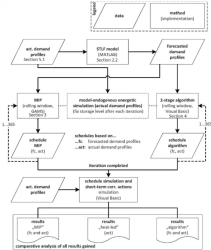
additional computing power and also satisfying the need of incorporating demand uncertainties. The methodological approach used in our case study focuses on applicable integrated methods to find a cost-minimized schedule for both the operation of a given domestic PEMFC micro-CHP unit and the charg-ing of an EV. In a preliminary step, this is achieved by load forecasting for each individual household and deterministic optimization meth-ods based on these individual point forecasts. The methodological approach is also outlined in Fig. 1.
1.3.1. Short-term Load Forecasting Approach
The first task is to address household-specific demand uncertain-ties, which is achieved by using a short-term load forecasting (STLF) approach based on the neuro-fuzzy model ANFIS (adaptive network based fuzzy inference system) (Jang, 1993). It is aimed at overcoming the lack of perfect information regarding near-future (day-ahead) demand patterns in reality by daily generating household individual (thermal and electric) point forecasts based on both historic data and exogenous influencing factors (weather, type of day, holiday indicator, etc.). Hence, the STLF approach addresses the uncertainties al-ready in a preliminary stage, which keeps the following optimization manageable even in highly decentralized systems
with low computing power and avoids the use of computationally expensive stochastic programming methods which would also cause the forecasting procedure to be much more complex. Our problem-specific implementation of ANFIS is described in Schönfelder, Jochem, and Fichtner (2012). Various other works successfully use ANFIS (cf. e.g. Ying & Pan, 2008; Yun, Quan, Caixin, Shaolan, Yumin, & Yang, 2008) or other methods, such as neural networks (Hsu & Chen, 2003) or support vector machines (Pai & Hong, 2005) for STLF purposes, mostly on a more aggregated level.
1.3.2. Optimization of Operation and Charging Schedules
The second task of our methodological approach is to create the
optimized operation and charging schedules based on forecasted demand patterns. For this purpose, an MILP (cf. Section 3.1) is defined
and implemented in a rolling window optimization fashion (cf. Section 3.2). Due to the common lack of sophisticated solver soft-ware in embedded systems, an additional algorithmic approach is developed, which is easy to implement and less computationally ex-pensive than the optimization approach (cf. Section 4). Consequently, it is better suited for the direct integration into real applications. Both methods integrate (energetic) model-endogenous simulation to fix storage levels deviating from reality in case of the occurrence of thermal forecasting errors after each iteration. This procedure is not necessary in reality, because the actual storage level can be measured directly before each iteration of the optimization. Due to the at least near-optimal solution generated by the MILP, it can also serve as a benchmark for the algorithmic approach. Furthermore, both methods can be also used with actual demand patterns instead of forecasted ones to define an upper bound for achievable savings for both of the optimization methods used (benchmark solution).
1.3.3. Simulation in Order to Consider Operation in Reality
Final results for each method are obtained in a third step by simu-lation runs in which the application of optimized schedules1 is simu-lated using actual demand patterns. Therefore, simulation represents the performance which could have been reached in an actual appli-cation. The simulation also includes rule-based application of short-term corrective actions, such as additional use of the backup (peak load) system in case of unforeseen thermal shortages or emergency shutdowns of the micro-CHP unit, if the thermal buffer storage system is filled unexpectedly, which very rarely happens due to forecasting errors (max. five times per year in our analysis). Hence, the simulation also represents online control in reality. To further improve the accuracy of simulation, actual demand patterns are synthesized to a temporal resolution of 1 minute (maintaining the boundary condi-tions given by the real demand patterns and using profiles in high resolution from VDI, 2008). This corrects averaging effects due to the use of discrete demand data in larger temporal resolution (cf. Section 3).
As a synopsis, the methods are finally compared with respect to their economic results within the framework of our case study (cf. Section 5). The results are additionally assessed with respect to their solutions’ quality depending on the method and quality of information (use of actual vs.
forecasted demand patterns). Section 6 concludes our findings and gives a critical review of our work.
As a synopsis, the methods are finally compared with respect to their economic results within the framework of our case study (cf. section 5). The results are additionally assessed with respect to their solutions’ quality depending on the method and quality of information (use of actual vs. forecasted demand patterns). Section 6 concludes our findings and gives a critical review of our work.
2. Micro-CHP Operating Strategies
The following section describes different approaches to scheduling micro-CHP units and their usability in real applications with the focus on PEMFC units. At first, we introduce the heat-led strategy, which serves together with equalized EV charging as the reference case in our case study.
2.1. Heat-led Strategy
In the case of a heat-led strategy, the operation of the micro-CHP unit is solely triggered by the thermal load of the building in which the unit is located. Assuming the presence of a thermal storage system, the signal for starting the operation of the CHP-unit is the drop of the thermal storage temperature below a specified lower temperature limit. Then, the unit works until the storage temperature reaches a specified upper limit again. The heat-led strategy is the most common operating strategy of micro-CHP units today (Schönfelder, 2013), as it meets the primary goal of covering the household’s thermal demand rather than deliv-ering electricity to it.
However, the legal situation in Germany favors own consumption of self-produced electricity in a direct (CHP bonus payment) and an indirect way (feed-in tariffs below purchase price of electricity) (Federal Republic of Germany, 2012).
2.2. Cost-minimizing Strategy
The economically optimized operating strategy is to provide for the supply of a local building with thermal energy and electricity at minimum
total operation costs2. The main variables of the optimization are the
electrical and thermal output power of the micro-CHP unit at each time step
t within the period under consideration T. Several parameters may be defined within an optimization model, such as variable electricity prices and feed-in tariffs, varying fuel prices, and technical restrictions of the unit like maximum cycles per time period, minimum up- and downtimes, ramp rates, and efficiency functions. However, as regards the level of technical detailing, a good compromise between accuracy of the results and the duration of the optimization has to be found in order to allow for an application in reality.
Apart from the parameters mentioned, the knowledge of the future temporal development of thermal and electrical demand of the considered household is crucial for the optimization. This is a major problem in practice, as these values vary as a function of the day, time, habits of the occupants, and many other properties of the household. Due to the lack of information, the cost-minimized strategy is often proclaimed in literature (Oh et al., 2012; Hawkes et al., 2006) but not yet implemented in practice. Our approach to STLF is based on demand patterns forecasted by our neuro-fuzzy model
Figure 2: Outline of the PEMFC micro CHP unit integration
2 Simply following the local electric load with the electric output power of the microCHP
ANFIS. All parameters of the adaptive nodes are part of the fuzzy inference system and modifiable during the learning procedure. As the accuracy of STLF increases with decreasing time horizon and term of the learning data, one iteration (learning based on recent load profiles and forecast of future load profile) per day seems to be suitable for our application. The scope of each forecasting iteration is at least 2 days. We use a multi-model approach (Hippert et al., 2001) with separate models for each type of day (regular working days, Fridays, Saturdays, Sundays, holidays). Training is based on historic data collected iteratively after the system’s installation. The scope of the training data set was determined by sensitivity analyses and is 12 days of the same type per model in our examples. More detailed information on our forecast model is given by Schönfelder (2013) and Schönfelder et al. (2012). 3. Economic Optimisation of the Unit Operation
The economically optimized operation of the CHP unit under consideration is defined to be the strategy with minimal operating costs that respects all techno-economic constraints. For the determination of the optimal unit operation, we use initially a MILP. The objective function comprises all relevant economic factors which are influenced by unit operation. The driving force of the MILP is (forecasted) local demand for thermal energy and electricity. Further constraints are formulated regarding technical properties of the PEMFC micro-CHP unit below. An outline of the system is given in Figure 2 and a comprehensive description can be found in Schönfelder (2013).
3.1. Mathematical Description
The following notations are introduced to formulate the problem.
Variables
B1CHP,t ) binary variable for the first (second) operating point of CHP in t
Bton binary variable indicating unit startup in t Btoff binary variable indicating unit shutdown in t Btc binary variable for counting operation cycles of CHP C total costs for household supply during T [e]
DtEV electric demand of the EV in t [kWh] Fecu,,tu′
LTSth,t
energy/material flow of ec from u ∈ U to u′ ∈ U in t [kWh]
level of thermal storage TS in t [kWh] energy supply ec in t at node node [kWh]
Parameters
process efficiency at node u regarding ec
maximum count of cycles per time period
demand for energy carrier ec in time step t (kilowatt-hour) length of each time step t (hour)
minimum downtime of the unit (given as number of timesteps) minimum uptime of the unit (given as number of timesteps)
Pecu,max maximum power at node u regarding ec (kilowatt)
pec,t price of ec in t (€ /kilowatt-hour) ρ power to heat ratio
σec,type,t subsidy type regarding ec in t (€ /kilowatt-hour)
Indexes Nodes
ec energy carrier BS thermal backup system
el electric D demand node
fit feed-in tariff EV electric vehicle
ng natural gas CHP PEMFC micro-CHP unit
oc own consumption Gr electricity grid
sl charging slot (EV) NG natural gas source
st start TS thermal buffer storage
stp stop Index Sets
t time step EC set of energy carriers ec tax energy taxes T set of time steps t th thermal SL set of charging slots sl u node U set of nodes u
The objective function of the MILP (equation (1)) minimizes the sum of all system-relevant costs of the operator in each time step t ∈ T, where T is the set of all time steps within the time horizon. Energy flows are denoted as
Fec,tu,u′, where ec ∈ EC indicates the energy carrier (ng=natural gas,
el=electricity, th=thermal energy). The model’s nodes to which the superscripts u, u′ ∈ U of energy flows refer are NG for the natural gas source,
Gr for the electricity grid, BS for the backup system, CHP for the PEMFC micro-CHP unit, TS for the thermal storage system, EV for the electric vehicle, and D for the demand. Time-flexible prices of energy carriers are labeled pec,t and specific subsidies from the operation of the unit are referred to as σec,type,t (type: oc=own consumption, fit=feed-in tariff, tax=tax savings). The operation of the micro-CHP unit is restricted in multiple respects. Besides the driving force of covering the thermal demand (constraint (2)), the model also has to ensure the coverage of the electrical demand either through local production or through the grid (constraint (3)). Concerning the demand restrictions, it is to be noted that the electrical demand of a possibly present EV DtEV is not a parameter, but a decision variable. Constraint (4) makes the model shift the charging process of the vehicle in an optimal manner with respect to individual temporal limits of each charging slot sl ∈ SL = {sl1,...,sln}
while covering the slot demand DslEV . The total charging demand DslEV of each charging slot sl ∈ SL as well as the individually associated quantity of time steps Tsl are exogenous parameters.
Thermal demands may be covered directly or through the storage system
TS. The model has to consider both the upper and lower (energetic) limit of the storage level (constraints (6) and (7)) as well as the (dis-)charging rate and storage efficiency ( out and ) according to constraint (5). The output power of the thermal storage system is not restricted due to the assumption that it is designed to meet the maximum thermal loads in the considered household.
Technical restrictions are defined regarding the power constraints of the micro-CHP unit and the backup system (constraint (8)) as well as in terms of maximum EV charging power (constraint (9)) for all time steps under consideration of time step’s duration ht. Further technical and physical
constraints are subject to the energy and material balances for all nodes u
and each energy carrier (constraint (10)).
A major cost driver is fuel consumption that depends on the operation and the efficiency ηtotCHP of the PEMFC micro-CHP and the backup system (constraints (11) and (12)). Due to the limited flexibility of PEMFC micro-CHP units, it is assumed that the unit allows for two fixed operating points (for our reference system these are 50 % and 100 % of nominal electrical power) apart from being switched off (constraint (13)). For modeling, binary variables B1CHP,t and B2CHP,t are implemented. The assumption of a fixed
relation of electrical to thermal power (power to heat ratio (ρ), constraint (14)) leads to the simplification that it is sufficient to limit the process level of one output energy carrier only (constraint (15)). Of course, these constraints can be adjusted easily when other micro-CHP technologies are studied.
The technological based minimum up- (¯τ) and downtimes (τ) of the PEMFC micro-CHP are defined in constraints (18) and (19) with the help of the binary variables Bton and Btoff indicating the start (in t = tst) and stop (in t
= tstp) of the CHP operation (constraints (16) and (17)). Because minimum
downtimes of the PEMFC micro-CHP are very low (τ = 1) (cf. Wakui and Yokoyama (2015)), constraint (19) was never binding. Therefore, we do not consider minimum downtimes τ in the following. Additionally, the technical restricted maximum number of cycles B¯c is considered where one cycle is defined as switch-on and complete switch-off (Btc) (constraint (20)).
3.2. Implementation as Rolling Window Optimisation
In the real application of the optimization problem defined in the previous section, several special circumstances have to be considered. Firstly, there is a considerable uncertainty regarding the future demand patterns of the household in which the PEMFC micro-CHP unit is located. This is addressed via the household individual load forecast (cf. section 2.2). However, even when utilizing point forecasting methods, there is only a short time horizon in which the demand is approximately known. Second, in case of an implementation of the methods described in an embedded system (preferably at low costs), limited computing power must be expected. This is mainly due to the goal of not significantly increasing the necessary investments for unit control. The solution of both problems is to perform the optimization in a repeated manner, e.g. once per day. This leads to permanently updated demand data and to a decreasing problem size (depending on the time horizon chosen). Technically, this way of optimizing
corresponds to a time-based decomposition of the global optimization into several static sub-problems (Bassett et al., 1996). Other decomposition techniques, e.g. disassembling the problem into multiple stages (cf. section 4), are likely to have higher negative effects, because the interdependencies between all parts of the problems are considerably strong. Also the global optimization for 1 year would neither be reasonable due to lacking information nor practicable, because the number of binaries (more than 140,000 binaries for one year in quarter-hourly resolution) would exceed common computing resources.
In connection with the given type of problem, there are two different ways of time-based decomposition:
(1) Construct several static and distinct sub-problems, e.g. daily optimization with the data of one day, or
(2) construct several overlapping sub-problems, e.g. daily optimization with a time horizon longer than 1 day.
Alternative (1) corresponds to the so-called myopic optimization (Chu, 1995; Ball, 2006) which neglects any data beyond the time horizon for which the operation is to be optimized. Hence, any influence of future demand patterns is ignored, which will obviously lead to suboptimal behavior in the sense of the global problem. For example, the optimization might stop CHP operation as soon as all remaining thermal loads can be covered by the storage system, which leads to thermal shortages at the very beginning of the following day. However, in Chu (1995) some other cases are discussed, in which a myopic approach does lead to global optimality or at least to the so-called near-optimality. Another problem of the myopic approach is that a small time window might cause infeasibilities although the global problem actually has feasible solutions (Bassett et al., 1996).
Alternative (2) describes the principle of a rolling window optimization (also called receding horizon optimization). Every sub-problem comprises several days and determines optimal operation for the given time horizon. However, only the schedule of the actual day remains as a fixed solution and the subsequent sub-problem will partly overwrite the solution determined the day before. Hence, consistency is achieved, because each optimization also takes future demand patterns into account (at least to the extent these are already known). The principle of rolling window optimization has been widely and successfully used in many areas (Li and Ierapetritou, 2010; Ovacik and Uzsoy, 1994; Zhang et al., 2007). An extensive overview and
classification of works on rolling window optimization and control is given in Chand et al. (2002).
4. Two-stage Algorithm for the Determination of Cost-effective Unit Operation
Due to the necessity of binary variables in the optimization model, the time and algorithmic effort to solve the model increase significantly compared to a purely linear problem. As the objective is to provide for an approach which is easily transferable to real applications, however, a simpler approach is desirably. Moreover, the long-term objective of an embedded system at low costs, which schedules the operation of the PEMFC micro-CHP unit, is associated with limited computing power and a lack of sophisticated solver3software in real applications. Therefore, we developed a two-stage
algorithm, which allows for the computation of a good operating strategy in a daily repeated manner, is easy to implement, and modest regarding the necessary computing power. In section 5 the results of both approaches (MILP and two-stage algorithm) are compared. Like the MILP, the two-stage algorithm can be used as a myopic or n-day rolling window approach (cf. section 3). The first stage of the algorithm is to determine an improved operation of the PEMFC micro-CHP unit (section 4.1). The second stage assigns an economically improved charging strategy for an EV. A complete integration of both scheduling tasks (micro-CHP and charging of EV) in one single stage is not reasonable in the algorithmic approach, as this would significantly increase the iterations necessary to compute a feasible solution. The algorithm is designed to use the household individual load forecasts based on ANFIS (cf. section 2.2). To also demonstrate the unaltered quality of results, however, besides forecasted demand patterns, also perfectly known actual data is used in the later analysis. This enables a detailed comparison of all variants and, hence, investigating both the influences of forecasting errors and the quality of the algorithm in comparison to the MILP. Furthermore, all techno-economic constraints described in section 3.1 are fully integrated in the algorithmic approach, although they are partly not mentioned again in the following sections. The following notations are used in the algorithm.
b time block of CHP operation PelCHP,t electrical power of CHP at time t
BtCHP level of CHP-operation PthCHP,t thermal power of CHP at time t
d set of days per iteration PthCHP,max max. thermal power of CHP [kW]
Dth,t thermal demand in t [kWh] Rt rate of t (Del,t · pel,t)
4.1. Stage 1: PEMFC Micro-CHP Operation
The algorithm’s first stage is designed to determine the daily operation of the PEMFC micro-CHP unit and consists of the mathematical implementation of rules which are easy to formulate in linguistic form. According to the number of days d considered and the applied temporal resolution of 15 minutes (ht = 0.25h), the count of set members in set T equals to d · 96. Furthermore, in all calculations within our case study we use a 2-day rolling window (i.e. we consider the actual and the following day). However, the algorithm is also compatible with higher
resolutions, e.g..
In the following sections the variable BtCHP represents the operation level of the CHP-unit. As valid points of operation, three different levels (0 %, 50 %, and 100 % of maximum power) are assumed, which are represented by
BtCHP ∈ {0,0.5,1}. The resulting electricity supply SelCHP,t is then calculated depending on the maximum electric power of the unit PelCHP,t and the length of the time steps ht (equation 23). Thermal supply SthCHP,t is determined accordingly (equation 24). Hence, BtCHP also represents the fraction of fullload operation in time step t. The number of full-load hours can therefore be computed as
Del,t electric demand in t [kWh] Rstb rate of block starting with tstb
DslEV total EV electric demand in sl Rmax highest rate of blocks considered
DtEV electric demand of EV in t [kWh] SthCHP,t thermal supply by CHP in t [kWh]
DEV,min min. EV electric demand for each t SelCHP,t electrical supply by CHP in t [kWh]
DEV,max max. EV electric demand for each t SL set of charging slots in T
ht length of time step t [h] T set of time steps t
level of thermal storage in t [kWh] sl charging slots sl ∈ SL LTSth ,max max. level of thermal storage in t tstb first t of block b LTSth ,min min. level of thermal storage in t teb last t of block b ¯τ min. operating time of CHP [h] tstsl first t of slot sl pel,t electricity price in t [e/kWh] tesl last t of slot sl
The first step of the algorithm is to determine whether the thermal demand of the following time steps t ∈ T minus the current thermal storage level does exceed the maximum thermal supply of the micro-CHP unit (in equation 25). If this is true, the unit is operated at maximum power for the next d · 96 hours (equation 26). LTSth,0 is the storage level at the beginning of time step t = 1 and
LTSth ,min is the minimum level of thermal storage in t. If additional thermal energy is needed temporarily, the backup system has to be put in operation as well (ensured with the last step of the algorithm).
If the first condition is false, there are degrees of freedom in the unit’s operation. Hence, the stored operational values BtCHP are initialized as zero (equation 27).
Now, it is to be checked whether a t∗ ∈ T ∗ exists, in which a thermal energy
shortage occurs. Accordingly, the whole considered time period is split up into (at least) two parts with part 1 ending in t∗ (cf. expression 31). Now, we
compute a ranking of the technically valid temporal blocks of operation within this first part equal to the minimum operation time ¯τ (given as a number of time steps). The minimum downtime is not binding and therefore not considered here. As depicted above, minimum downtimes τ of the PEMFC micro-CHP units are neglected here, as they are not relevant for this technology. The blockwise rates Rstb, which are based on the stepwise rates
with T˜ = {t ∈ T|t + ¯τ ≤ t∗} and ending at teb = tstb + ¯τ. The stepwise rates Rt are
defined as the product of the entire local electricity demand in time step t and the (possibly time-dependent) electricity price pel,t. This considers already the simplified equalized electricity demand by EV during the charging slot (SL starting at time step tstsl and ending at tesl) (cf. expression 34). This way of
deriving the stepwise rates ensures the compatibility of the algorithm with time-flexible electricity prices. Based on the block ranking of all eligible blocks in this first part of the considered time period, we choose the best rated one (maximum rate) to run the micro-CHP unit (expressions 32-37). Hence, the variable BtCHP, indicating the operation level of the unit, is increased for the best rated block beginning in time step tstb (BtCHP is restricted to a maximum value of 1). Then, the values of BtCHP are stored to
BˆtCHP and the procedure is repeated iteratively. The rates and ranks are updated before the next iteration until no further shortage occurs or no further degrees of freedom exist. The algorithm is not only able to add new blocks of operation, but also to extend those blocks already planned in previous steps (which then means a block of operation longer than ¯τ). In case of missing degrees of freedom, the backup system is used to provide the thermal energy lacking (determined in the last step of the algorithm).
The following step of the algorithm (expressions 38-43) is applied, if no or no further thermal energy shortage occurs but the minimum total operating time is not yet reached and, hence, degrees of freedom still exist. This step is especially relevant, if high degrees of freedom exist, e.g. in summer months. Together with the previous step, this is the key difference to the heat-led strategy commonly used today.
In this situation, where the minimum total operating time is not yet reached, a block ranking is calculated again. However, now the entire time horizon is considered. Based on the ranking, those operating times are preferred, which promise a high rate of own consumption of locally produced electricity or which have the highest ranking based on time-flexible electricity prices. This is equivalent to the goal of economic improvements from the investor’s point of view.
Once more, an iterative approach is selected to supplement the blocks of operation with further time steps or to add whole blocks of operation. The iteration ends as soon as the minimum operating time, necessary to cover the heat demand of the considered days, is reached.
then calculate for all t ∈ T the corresponding rates Rstb
In the last step of the first stage all remaining thermal shortages are treated through the operation of the backup system. Furthermore, it is checked whether one or more time steps t¯exist, in which the maximum thermal storage level LTSth ,max is exceeded. In this case, the operation of the PEMFC micro-CHP unit is adapted accordingly. In an iterative approach the algorithm sanctions the time steps t ≤ t¯ with the lowest stepwise rates so that the operation is shifted to the time after the storage level is exceeded. By a repetition of the algorithm’s first stage, the validity of the new solution is ensured.
After the completion of the algorithm’s first stage, the second one is applied to determine an improved charging strategy for the EV compared to the equalized strategy assumed in algorithm one. This second stage is described in the following section.
4.2. Stage 2: EV Charging
Monotonous charging of the EV (i.e. charging the required electricity during the whole parking time at constant (low) load) assumed in the first stage of the algorithm is not necessarily economically advantageous. However, a simultaneous determination of optimal operation of the micro-CHP unit and optimal charging of the EV is highly complex and requires high computing time. Hence, a simple stepwise approach is selected on the
algorithmic level. The first assumption of monotonous charging increases the probability of the unit operating in times when the EV is present. Possible degrees of freedom regarding the charging process are generated and now utilized with the second stage of the algorithm.
In the first step of stage 2 the number of charging slots SL in the considered time horizon is detected. If the number is higher than zero, the limits (begin tstsl and end tesl) of each temporal slot are determined and the aggregated electrical demand of the EV DslEV of each slot sl ∈ SL is calculated with the assumption of full charging, if possible (equation 45). If |SL| = 0, the algorithm ends, because either the household is not equipped with an EV or the EV is not present in the considered time horizon or there is no need for charging, because the battery already is fully charged. Again, for algorithmic reasons, the slot demands are stored in the auxiliary variables DˆslEV .
The second step of the algorithm calculates the times to charge the EV for every slot sl in a way which maximizes the own consumption of the locally produced electricity SelCHP,t in each time step t ∈ {tstsl,...,tesl}. Potentially time-flexible electricity prices are only considered, if no further own consumption can be generated. This is due to the assumption, that own consumption is generally preferable, if possible. The algorithm now plans the charging process of the EV with respect to technical constraints, such as minimum and maximum charging power (expressed by minimum DEV,min and maximum
DEV,max energy per time step) as well as in accordance with the requirement of charging the vehicle as soon as possible, if no further economic advantages can be generated (p′el respresents the lowest possible charging tariff in
compliance with technical constraints). Again, the algorithm is implemented as an iterative approach performed for each charging slot sl ∈ SL according to the equations below (expressions 47-53). The iterations are stopped when the maximum electricity demand by EV DslEV is satisfied for all charging slots.
Since the results of the algorithm are valid integer solutions, they can also be used as starting solution for the MILP described in section 3. Usually, this accelerates the solution process of the MILP, especially if long time horizons for the sub-problems are applied. In contrast to the first stage of the algorithm (cf. section 4.1), the second stage (EV charging) assumes a perfect foresight for the availability of the EV. The resulting costs could be therefore interpreted as a lower bound.
5. Application and Results
The application of both the two-stage algorithm and the MILP in our case study is to analyze the economic benefits from both methodologies and to compare them to the results from the standard heat-led strategy and monotonous charging of the EV. Furthermore, we compare the computing time of both approaches. For the results of the case study to be perfectly
comparable, the analysis is performed both based on forecasted demand patterns (based on our STLF approach) and under the assumption of perfectly knowing future demand patterns in advance (each in quarter-hourly temporal resolution). Using forecasted demand patterns as input for the optimisation represents the realistic case, while the use of actual demand data prevents disturbing influences of possible forecasting errors and allows for a principle statement regarding the solution quality of the two-stage algorithm. The quality measure is the percentage deviation from the benchmark solution which is calculated by solving the MILP. In total, there are four different methodological variants to be analyzed per household:
1. MILP (act): MILP based on actual demand data to calculate a schedule representing a benchmark for all other versions,
2. MILP (fc): MILP based on forecasted demand patterns to present the MILP’s results under realistic uncertainty conditions (benchmark for 4.),
3. Alg. (act): two-stage algorithm based on actual demand data to calculate the best possible schedule delivered by the algorithm (can be compared to 1. to evaluate the quality of the algorithm),
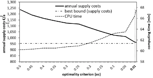
4. Alg. (fc): two-stage algorithm based on forecasted demand patterns topresent the algorithm’s results under realistic demand uncertainty. The MILPs are implemented in the modeling system GAMS (General Algebraic Modeling System (Corporation, 2012)). The solver used is CPLEX 12.0 (IBM, 2012) which applies the branch-and-cut algorithm for the solution of the MILP sub-problems. Every sub-problem includes 2,075 real-valued variables, 760 binaries, and 1,592 restrictions. As the proof of optimality for MIP problems can be very expensive because they are NP-hard (Karp, 1972; Tseng, 1996), we applied a relative optimality criterion oc = 0.01 as a good compromise between quality of the solution and computing time. This means that an integer-feasible solution with a deviation of 1 % from the actual dual bound is accepted as optimal. To illustrate the effects of the selection of the optimality criterion, we varied it in a typical application for household 2, as presented in Figure 3. While the value of the objective function decreases approximately linearly, the computing time ct increases rapidly for very small values of the optimality criterion. In our test runs no solution was found after 20 hours of computing time with oc < 0.005. Hence, we found oc = 0.01 to be the best compromise between quality of the solution and computing time. We carried out all experiments in a 64 bit Windows 7 environment on a 3.3 GHz Quad Core machine with 16 GB of RAM. The computing time with
the applied relative optimality criterion oc = 0.01 amounts to about 66 minutes for the MILP.
Figure 3: Annual supply costs for an illustrative household and computing time for one year depending on the relative optimality criterion.
The rolling window approach (cf. section 3.2) with a time horizon of two days shows significantly lower annual supply costs of households as a time horizon of one day and only very marginal higher costs as larger time horizons. Simultaneously, the computing time and the number of binaries per sub-problem both increase linearly with increasing numbers of days considered (Sch¨onfelder, 2013). We, therefore, applied the 2-day rolling window approach.
Final results for all variants are derived using the simulation as described in section 1.3 and including all additional short-term corrective actions necessary due to forecasting errors. To evaluate economic effects, all results are compared with those of the standard case of the heat-led strategy. The definition of error and quality measures capturing all dimensions of the comparison of different variants is given in section 5.2 in connection with the results.
5.1. Assumptions and Data
Our case study comprises the two exemplary households defined in Table 1. Each of these households is represented with thermal and electrical demand data of 1 year. These two households are chosen to represent the main target group of PEMFC micro-CHP units in Germany, namely small and
medium-sized households with aver-age heat demand (Federal Republic of Germany, 2009). Besides the different sums of yearly electricity demand, the yearly heat demand is given per household, which results in slightly differing degrees of freedom for the unit commitment. The system specifications of the PEMFC micro-CHP unit have been defined before and satisfies all requirements (cf. Schönfelder, 2013). The operation of the CHP in both households is once optimized with the presence of an EV and once without. Its electricity demand is derived from a measured driving profile and amounts to 2549 kilowatt-hour per year (IIP, 2012). This corresponds to an annual mileage of approx. 13,000 kilometer. The mobility pattern is compliant with representative German mobility surveys (Infas, DLR, & DIW, 2010; KIT & TNS, 2012). The thermal demand patterns are derived using actual weather data from Germany’s meteorological service (DWD) and according to the calculation rules from VDI (2008) indicating values with a temporal resolution of up to 1 minute. Electric load profiles were measured in 66 real German households over 1 year with quarter-hourly temporal resolution (IIP, 2012). Out of this data set we selected two profiles matching the average annual electricity demand of households of the considered size. Furthermore, the variants defined are analyzed both with constant and time-flexible electricity tariffs. The latter is to demonstrate the optimization methods’ ability of utilizing time-dependent differences in electricity prices by adapting both the operation and the charging schedule. In total, the two different households, the distinction be-tween the presence or absence of an EV, and the differentiation of a constant and time-flexible tariff structure lead to a total of eight variants (cf. Table 2) which are investigated with two different optimization methods (MILP and Algorithm) and two different qualities of information (actual and forecasted demand patterns).
Demand forecasting with the ANFIS model (cf. section 2.2) results in overall median absolute percentage errors (MdAPE) of MdAPEel,hh1 = 13 %
and MdAPEel,hh2 = 22 % for the electrical forecasts and MdAPEth ≈ 15 % for
both thermal forecasts. Compared to STLF on an aggregated level, these error values, which also nearly represent the range of errors in the whole case study considering four households in total4, are not completely satisfying.
However, they are due to the highly fluctuating demand structure of single households and, hence, have to be judged according to these special circum-
Table 1: Definition of two test households with hh2 being better insulated than hh1.
Heat demand Electricity demand Household Living space Residents per year per year
hh1 90 m2 2 13,538 kWh/a 2,845 kWh/a
hh2 120 m2 3 10,891 kWh/a 4,385 kWh/a
stances. Nevertheless, the following analyses will show that the forecasting quality is good enough to allow for major improvements in the operation of the micro-CHP unit. This is mainly due to the fact that exactly meeting absolute values is not as important as correctly anticipating rough times of high household demand in our application. Yet, it is clear that positive effects are finally dependent on the overall forecasting quality. Certainly, there are households in which the proposed methods fail when they are not adapted to special circumstances. For example, this could be necessary in shift workers’ households with a stochastic shift distribution. Further limitations of our approach are discussed in section 6 in the form of a critical review.
The reference system considered for both households is a PEMFC-based micro-CHP unit with a maximum electric power of 1.2 kWel. The system’s output power is chosen to fit the annual thermal demand of both houesholds, resulting in approx. 5,000 annual full load hours. This corresponds to well-established dimensioning rules for fuel cell-based micro-CHP units in Germany (Thomas, 2011). The PEMFC unit used in our case study is highly efficient compared to other technologies like CHP systems based on gas engines for example, but still suffers from its high price and its limited flexibility which is mainly due to the necessity of decentralized conversion of natural gas into hydrogen (Thomas, 2011; Pehnt et al., 2012). This is reflected by a minimum operation time which is assumed to be 2 hours (= 8 time steps) as well as by fixed operating points at 0, 50, and 100 % of the nominal power. The overall efficiency of the unit is ηchp = 0.91. As described above, household electricity prices are estimated conservatively and assumed to be either constant over the entire time horizon (pel,t = 0.25 e/kWh ∀t ∈ T) or time-dependent (pel,t ∈ {0.18,0.25,0.32} e/kWh) with a tariff structure inspired by Gerpott and Paukert (2013) and exogenously given depending on the residual grid load (grid load minus feed-in of non-controllable renewable energy sources). The latter tariffs are likely to become more common in the near future due to the necessity of better integrating fluctuating feed-ins from renewable energy sources (Hirsch et al., 2010). Other economic parameters like natural gas prices (png = 64.3 e/MWh) or CHP bonus
payments (σel,oc = 0.0541 e/kWh) (Federal Republic of Germany, 2012) correspond to current market values for residential customers in Germany.
5.2. Numerical Results
The following sections describe numerical results for the two illustrative households defined in Table 1. Computing times for the MILP and the algorithmic approach are rather constant for all scenarios due to similar problem sizes. The differences between energy economic values are, however, substantial.
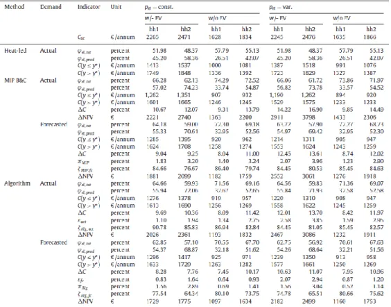
Table 2: Comparison of the energy economic results for different methods and different qualities of information (actual=using actual demand patterns, forecasted=using forecasted demand patterns). End of the funding period according to Germany’s CHP Act (Federal Republic of Germany, 2012) is marked as y∗.
Cuc: annual costs of uncoupled supply; C(y ≤ y∗)/C(y > y∗): annual costs before/after the end of funding period (10
years of bonus payments according to CHP act (Federal Republic of Germany, 2012)); ∆C: change of C(y ≤ y∗) compared to heat-led operation; ∆NPV: change of NPV compared to heat-led operation; φel,tot: fraction of the
household’s total el. demand covered by the micro-CHP unit; φel,prod: fraction of the micro-CHP’s total el. production
5.2.1. Yearly Absolute Savings due to the Optimisation
The absolute values of the results given in Table 2 show that the coupled generation of heat and electricity is advantageous for both households considered, even with the heat-led strategy compared to the uncoupled supply (Cuc, representing household supply with electricity solely from the grid and thermal energy from a decentral heating based on natural gas). However, this does not guarantee any positive net present value (NPV) in total, because only operational costs, but not the investments are considered in this analysis. Furthermore, the analysis reveals that the schedules determined by the MILP or by the two-stage algorithm result in lower annual costs than in case of the heat-led strategy. Obviously, the positive effects strongly depend on the degrees of freedom in the unit commitment. The slightly lower total thermal energy demand of hh2 combined with its higher electricity demand results in the possibility of larger improvements than in hh1. Consequently, slightly oversized units will profit more from the optimization, while undersized units might be better driven heat-led, because no significant improvements are to be expected. Summing up the results of our case study with the well-dimensioned system, yearly savings (∆C) of about 7.5 to 16.9 % are possible, which mainly depends on the method and the quality of information (actual vs. forecasted data) used. Here, all short-term corrective actions (determined in the simulation of the schedules) which would have been necessary in a real application are already included. For example, for hh2 and the schedule derived by the algorithmic approach based on forecasted demand patterns, the simulation calculates an increase of the backup system’s application due to thermal forecasting errors of approx. 5 % compared to the value originally stated by the two-stage algorithm. Furthermore, compared to unaltered algorithmic results (where forecasts are assumed to be
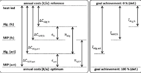
Figure 4: Developed and applied error measures. The values of π and ϵ are defined as relative values as defined in the equations 55a,b and 56a,b.
correct), the simulation shows increasing electricity purchase from the grid of approx. 7 % which results in an equivalent unexpected feed-in of locally produced electricity and, hence, a decrease of own consumption. The latter is the main reason for the difference of economic results between optimisation based on actual and forecasted demand patterns.
5.2.2. Assessment of Scale-transformed Results
Beside absolute values, Table 2 also provides energy economic performance indicators regarding the scale-transformed (percentage scale) loss of the solution’s quality due to the use of a non-optimal algorithm and due to forecasting errors. The latter also includes economic impacts of all
short-term corrective actions described above. Consequently, error measures are introduced as depicted in Figure 4. Starting point for the calculation of the change of annual costs (∆C) is the reference case of heat-led strategy. ∆C is given separately for each combination of method and quality of information. The loss due to forecasting errors is expressed by π as a percentage for both methods. However, the comparison of πMIP and πAlg does not necessarily reveal whether one of the two methods handles forecasting errors better than the other due to the different reference values. Nevertheless, it gives interesting information on each method’s individual sensitivity to the forecast errors. The third error measure ϵ is defined relatively to the MILP solution serving as a benchmark for the given quality of information. ϵact and
ϵfc express to what an extent the annual costs calculated in the simulation of the schedule determined by the algorithm deviate from the corresponding value of the MILP schedule. Together, π and ϵ explain the overall loss due to imperfect information on future demand patterns and the non-optimal solution of the two-stage algorithm. Furthermore, a measure ζ is used to evaluate the overall goal achievement of one method relative to the ex-post optimal solution given by the MILP’s solution based on actual demand data. Mathematical definition of all measures mentioned is given in the following set of equations.
The values of πMIP range between 1.2 and 4.0 %, while πAlg lies between 0.52 and 3.0 % (cf. Table 2) and therefore the two-stage algorithm perform similar with forecasting errors than the MILP. However, due to its non-optimal solution in general, its total performance is, as expected, slightly worse than for the MILP. The latter is expressed by the values of ϵact between 1.1 and 3.8 % and ϵfc ranging between 0.64 and 2.94 %. The presence of an EV increases these differences because the two-stage algorithmic planning approach is, compared to the MILP, less able to take interdependencies between CHP scheduling and EV charging into account. While the relative goal achievement of the algorithm is at least closer to the result of the MILP than to the heat-led strategy (ζAlg,fc between 64.3 and 80.7 %), the value is considerably higher for the perfect foresight scenario (ζAlg,act between 81.05 and 90.78 %). The average computing time on a desktop computer could be reduced from about 66 minutes for the MILP (cf. section 5) to about four minutes for one year optimization on the average for the algorithm for all eight variants considered. Even though the computing time might be somewhat higher for low-cost embedded systems, our approach seems to be very promising for real applications.
Comparing the standard case of the heat-led strategy and the operation based on the algorithmic optimization on a monthly basis in hh2 with the assumption of a constant tariff, it becomes obvious, that the amount of electricity produced each month strongly depends on the corresponding thermal demand which directly determines the maximum time of CHP operation. A rough classification of the months leads to three substantially different phaseswhich are mainly weather-dependent. The first one is the
winter period with a high thermal demand, mainly due to the requirement of
heating the household. The micro-CHP unit normally operates at full power throughout this period. There are hardly any degrees of freedom to be exploited by the optimization, which is why only few positive effects can be generated. Another period in which the optimization is barely able to generate improvements is the summer period. This is due to a thermal household demand near to zero (only for warm water), which means that the CHP-unit is hardly run and, hence, does not produce much electricity. The third period may be classified as transition period and is characterized by constantly decreasing (between winter and summer) or increasing (between summer and winter) thermal demand. This period provides significant degrees of freedom regarding the operation and, hence, the potential for generating positive effects in terms of increasing the share of own consumption (marked as φel,prod in Table 2). Furthermore, the presence of an EV seems to have positive effects on the own consumption rate in all seasons due to the increase of the household’s total electricity demand.
6. Conclusions and Critical Review
We presented a case study based on a comprehensive approach to determining improved residential PEMFC micro-CHP operating strategies. As information about the short-term local demand patterns is imperfect in real applications, we used an STLF model (cf. section 2.2). It is based on ANFIS addressing the demand uncertainty in a first stage via so-called point forecasts representing the most likely realization of the short-term local demand. Subsequently, both an MILP and a two-stage algorithmic method were presented. They use the point forecasts to derive economically optimized schedules in a rolling window optimization fashion. Hence, we address demand uncertainty by load forecasting instead of using stochastic programming, as it is more realistic for real applications. The schedules derived in a daily repeated manner are then analyzed in a simulation using actual demand patterns in a temporal resolution of one minute to derive all necessary short-term corrective actions and, hence, the performance which
could have been realized in the real application. The results obtained with the schedule generated by the algorithmic approach in our case study mostly deviated by less than 3 % from those of the MILP’s integer optimal solution and computing time could be reduced by a factor of 15. Furthermore, the two-stage algorithm might have further advantages in being implemented in current PEMFC micro-CHP units and not to be dependent on sophisticated hardware and solver software and therefore operating more reliable than MILP based systems during the unit lifetime of about 20 years.
However, the absolute advantages generated by both approaches compared to the standard case of heat-led operation strongly depend on the individual household’s characteristics. If only few degrees of freedom in unit operation exist, it might be easier to apply the heat-led strategy (e.g. in winter months). Nevertheless, especially in transition periods and with the presence of an EV, the methods developed yield significantly improved solutions. For example, for an illustrative household in our case study, overall discounted savings of approximately 2,500 e were reached compared to the heat-let strategy using forecasted load patterns under the assumption of time-flexible electricity prices. This is equivalent to nearly twice the current governmental funding for PEMFC micro-CHP units at 1.2 kWel in Germany (BMUB, 2012), while the electricity prices used in our case study were estimated very conservatively. As the results are quite sensitive to the electricity price, increasing prices will further enhance the positive effects achieved.
It should be noted that the effects achieved by the application of the methods used depend on the quality of the forecast demand patterns. In turn, the quality of the forecast strongly depends on the individual household’s characteristics (Schönfelder, 2013). Certainly, some households are not suited for the application due to highly differing demand patterns which are not predictable with the STLF models. This may be a household in which all residents are shift workers who do not always follow fixed shift plans. The analysis also revealed, however, that the rough prediction of household-specific peak load times often already allows to significantly improve the operation of the PEMFC micro-CHP unit. Nevertheless, further enhancement of the forecast quality is likely to intensify positive economic effects. The upper bound of these positive effects is given by the assumption of perfectly knowing the actual demand in advance.
Another weakness of the developed methods is the fact that the results obtained, even if they are positive, do not necessarily mean that the installation of a PEMFC micro-CHP unit generally is economically
advantageous compared to uncoupled supply. Moreover, due to the case study character of our investigation, the results are not necessarily generalizable.
References
Ball, M., 2006. Integration of a hydrogen economy into a national energy system using Germany as an example: Options for hydrogen supply as fuel for road vehicles until year 2030 (published in German language: Integration einer Wasserstoffwirtschaft in ein nationales Energiesystem am Beispiel Deutschlands: Optionen der Bereitstellung von Wasserstoff als Kraftstoff im Straßenverkehr bis zum Jahr 2030). VDI Publishing.
Bassett, M., Pekny, J., Reklaitis, G., 1996. Decomposition techniques for the solution of large-scale scheduling problems. AIChE Journal 42 (12), 3373– 3387.
BMUB, 2012. Guidelines for the funding of CHP-units up to 20 kWel (published in German language: Richtlinien zur F¨orderung von KWK-Anlagen bis 20 kWel). German Federal Ministry for the Environment, Nature Conservation and Nuclear Safety (BMUB).
Boait, P., Rylatt, R., Stokes, M., 2006. Optimisation of consumer benefits from micro Combined Heat and Power. Energy and Buildings 38 (8), 981– 987.
Bosman, M., Bakker, V., Molderink, A., Hurink, J., Smit, G., 2012. Planning the production of a fleet of domestic combined heat and power generators. European Journal of Operational Research 216 (1), 140–151.
Carøe, C., Schultz, R., 1998. A two-stage stochastic program for unit commitment under uncertainty in a hydro-thermal power system. Konrad-ZuseZentrum fu¨r Informationstechnik Berlin (ZIB), Berlin.
Carøe, C., Schultz, R., 1999. Dual decomposition in stochastic integer programming. Operations Research Letters 24 (1), 37–45.
Chand, S., Hsu, V., Sethi, S., 2002. Forecast, solution, and rolling horizons in operations management problems: A classified bibliography. Manufacturing & Service Operations Management 4 (1), 25–43.