I
OWAS
TATEU
NIVERSITYDepartment of Economics
Ames, Iowa, 50011-‐1070
Iowa State University does not discriminate on the basis of race, color, age, religion, national origin, sexual orientation, gender identity, genetic information, sex, marital status, disability, or status as a U.S. veteran. Inquiries can be directed to the Director of Equal Opportunity and Compliance, 3280 Beardshear Hall, (515) 294-‐7612.
Do Gender Differences in Risk Preferences Explain
Gender Differences in Labor Supply, Earnings or
Occupational Choice?
In Soo Cho
Working Paper No. 11022 December 2011
Do gender differences in risk preferences explain gender differences in
labor supply, earnings or occupational choice?
Insoo Cho
Abstract
This paper examines the extent to which differences in risk preferences between men and women explain why women have a lower entrepreneurship rate, earn less, and work fewer hours than men. Data from the NLSY79 confirms previous findings that women are more risk averse than men. However, while less risk averse men tend to become self-employed and more risk averse men are likely to choose paid-employment, there is no significant effect of risk preferences on women’s entrepreneurship decisions. Similarly, more risk aversion is associated with higher earnings for male entrepreneurs, but it has no effect on female entrepreneurial earnings. Rising rates of risk aversion lower earnings for women, consistent with theoretical effects of risk preferences on labor earnings, but the effects are of modest magnitude. Risk preferences do not explain variation in hours of work for either men or women. These findings suggest that widely reported differences in risk preferences across genders play only a trivial role in explaining differences in labor market outcomes between men and women.
Key words: risk aversion, gender gap, self-employment, earnings, labor supply, Blinder-Oaxaca decomposition
JEL Classifications: J24, J22, J31, J16
______________ ___
Department of Economics, Iowa State University, Ames, IA 50011-1070 USA. Cho: [email protected]
1. Introduction
On average, women are less likely to become self-employed, earn less and work fewer hours than men. While a vast literature has investigated the extent to which these gaps can be explained by differences in human capital, a more recent effort has found that noncognitive skills such as emotional stability, conscientiousness and aggression or antagonism can explain some of the pay differences between men and women (Mueller and Plug, 2006).
Numerous studies have found that women are more risk averse than men (e.g., Barsky et al., 1997; Hartog et al., 2002; Eckel and Grossman, 2008; Borghans et al., 2009; Croson and Gneezy, 2009). Recent experimental studies found that women do not perform as well as men in competitive environments (Gneezy et al., 2003; Niederle and Vesterlund, 2007; Croson and Cneezy, 2009). One might presume that gender differences in labor market outcomes would be partially explained by such differences as well.
In fact, risk preferences are commonly found to have a significant role in determining entry into self-employment for men(Van Praag and Cramer, 2001; Hartog et al., 2002; Cramer et al., 2002; Ekelund et al., 2005; Kan and Tsai, 2006; Ahn, 2009). Bonin et al. (2007) find that the least risk averse individuals select occupations with higher wages and higher variation in wages. It is tempting to presume that women’s greater aversion to risk and competition explains women’s lower wages and lower rate of entrepreneurship, as suggested by Croson and Gneezy (2009). However, that link has not yet been established empirically. To date, most studies of labor market outcomes tied to risk preferences have relied either on cross sectional data sets of men only or of pooled samples that do not estimate separate effects of risk preferences
across genders.
The exception is a study of the gender wage gap in Australia by Le et al. (2010) which found that favorable attitudes toward financial risk raises earnings for both men and women. However, gender differences in risk attitudes explain only a small part of the gender pay gap. To our knowledge, no previous study has investigated the extent to which risk preferences explain gender gaps in occupational choice or labor supply. This study examines the role of risk preferences in explaining observed gender gaps in entrepreneurship, earnings and hours worked in the 1979 National Longitudinal Surveys of Youth.
Consistent with the earlier studies, we find that less risk averse men are more likely to enter self-employment. However, we find no significant effect of risk attitudes on women’s entrepreneurship. The role of risk aversion also differs by gender across employment type. In self-employment, less risk aversion is associated with lower male earnings, but risk aversion has no effect on female earnings. In paid-employment, less risk aversion lowers male wage whereas it raises female wage. Finally, we find no relationship between risk aversion and hours of labor for both men and women. Consequently, a standard decomposition shows that gender differences in risk attitudes explain only a small fraction of the gender gap in self-employment. Similarly, those differences in risk aversion between men and women account for only a trivial portion of the gender gap in earnings and hours worked.
The structure of the paper is as follows. Section 2 describes conceptual frameworks for the relationship between risk aversion and occupational choice, earnings, and work effort in hours. In section 3, empirical methodology and data are discussed. In the subsection, the measures of individual risk attitudes are briefly
summarized. Section 4 shows empirical results, along with results of the Blinder-Oaxaca decomposition for both non-linear and linear models. The following subsection shows results of sensitivity analysis. Section 5 concludes.
2. Conceptual framework: Choosing occupation, earnings and hours of labor
This section shows that in theory, risk preferences should affect individual decisions regarding labor force entry, occupation and earnings conditional on entry, and hours of work. Consequently, differences in risk preferences between men and
women potentially could explain some of the gender differences in these choices. Individuals are assumed to choose one of three employment types:
self-employment, paid self-employment, or being out of labor force so as to maximize expected utility. Utility depends on expected pecuniary returns from market work and utility from nonmarket work or leisure. Utility is concave in earnings so that it can reflect an individual’s risk aversion. Individuals form their beliefs of future earnings based on their human capital which contributes to his/her productivity at home or on the job. The reduced form utility function from an individual i choosing an employment type j is given by ( , , , ) ij ij ij iL i U =F e y μ θ (1) ( ) ij mi y = f X (2) ( , ) iL f Xmi Xhi μ = (3) where eijis work effort in j occupation (i.e., fraction of time spent in j); ~yij denotes
affects ability in the market; μiLis known utility from nonmarket work which is determined byXmi and factors that influence productivity in home production, Xhi;
and θi denotes a measure of i’s risk aversion.
Following Barsky et al. (1997) and Kimball et al. (2008), we assume that individuals have constant relative risk aversion (CRRA). The associated utility function from employment type jis given by:
1 ( ) (1 ) 1 i ij ij ij ij iL ij i y U e e θ μ ε θ − = + − + − , θ 1 (4) where ( ) 0 ( ) ij ij i ij y U y U y θ =− ′′ > ′
is the Arrow-Pratt measure of the coefficient of individual
i’s relative risk aversion; (1-eij) denotes fraction of time spent in the home; εi is an
error term which captures unobservable factors such as motivation and preferences for job attributes.
In order to derive expected utility with respect to future earnings, we take a second order Taylor series expansion around the mean of future earnings (μ~y). For
simplicity, the subscripts i and j are suppressed:
2 1 ( ( )) ( ) ( ) ( ) ( ) (( ) ) 2 y y y y y E U y ≈U μ +U′ μ E y−μ + U′′ μ E y−μ +ω ( ) 1 ( ) 2 2 y y y U μ U′′ μ σ ω = + + (5) where μ~y =E(~y), σy2~ =Var(~y), and ω is a random error due to approximation.
The first and second order partial derivatives of the equation (4) with respect to
y
~ are respectively: ( ) ( )
1
( ) ( )
U y′′ = −e yθ − −θ (6) Plugging equations (4) and (6) into equation (5) yields
1 1 2 1 ( ) (1 ) 1 2 y y y L E U e e θ θ μ θμ σ μ ω ε θ − − − ⎛ ⎞ ≈ ⎜⎜ − ⎟⎟+ − + + − ⎝ ⎠ (7)
An individual optimally allocates time between market work and nonmarket work by maximizing his expected utility with respect to work effort, e. The first order condition is given by (8) EU e ∂ ∂ 0 2 1 1 1 2 y y L y θ θ σ μ μ θ μ − ⎛⎜ ⎛ ⎞ ⎞⎟ ⇔ − ⎜⎜ ⎟⎟ − ⎜ − ⎝ ⎠ ⎟ ⎝ ⎠ 0 (8) * 0 e > if 2 1 1 1 2 y y L y θ θ σ μ μ θ μ − ⎛⎜ − ⎛ ⎞ ⎞⎟= ⎜ ⎟ ⎜ ⎟ ⎜ − ⎝ ⎠ ⎟ ⎝ ⎠ (9) * 0 e = if 2 1 1 1 2 y y L y θ θ σ μ μ θ μ − ⎛⎜ − ⎛ ⎞ ⎞⎟< ⎜ ⎟ ⎜ ⎟ ⎜ − ⎝ ⎠ ⎟ ⎝ ⎠ (10) * 1 e = if 2 1 1 1 2 y y L y θ θ σ μ μ θ μ − ⎛⎜ − ⎛ ⎞ ⎞⎟> ⎜ ⎟ ⎜ ⎟ ⎜ − ⎝ ⎠ ⎟ ⎝ ⎠ (11)
Equations (9), (10), and (11) show that if expected utility from earnings in the market at any positive e equals utility from nonmarket work or leisure, an agent allocates his available time between market work and nonmarket work (e* >0); Otherwise he will specialize in home production (e*=0) or market production (e*=1). Clearly, a decision on whether to enter the labor market depends on risk attitudes, human capital, and household characteristics so that e* =e( ,θ X Xm, h).
In addition, if we presume that the utility from time out of the labor force is positive (μL >0)then an interior solution where 0<e<1 requires that
2 1 1 1 2 y y y θ θ σ μ θ μ − ⎛⎜ − ⎜⎛ ⎞ ⎞⎟ ⎟ ⎜ ⎟ ⎜ − ⎝ ⎠ ⎟ ⎝ ⎠
>0. That in turn requires that the risk aversion parameter
(0,1) θ∈ and 2 1 2 1 y y σ θ μ θ ⎛ ⎞ < ⎜ ⎟ ⎜ ⎟ − ⎝ ⎠
.1 For the rest of our analysis, we will presume that
for individuals in the labor market, 0 < θ< 1.
Assuming e>0, an individual chooses self-employment if expected utility from selecting self-employment exceeds that from paid-employment:
0 0
|
s|
ws e w e
EU
>>
EU
>Manipulating expected utility yields the following condition for entering self-employment: 2 2 , , 1 1 , , , , 1 1 (1 ) (1 ) 1 2 1 2 y s y w s y s s L w y w w L y s y w eμ θ θ σ e μ e μ θ θ σ e μ θ μ θ μ − ⎢⎡ − ⎜⎛ ⎟⎞ ⎥⎤+ − > − ⎢⎡ − ⎛⎜ ⎞⎟ ⎥⎤+ − ⎜ ⎟ ⎜ ⎟ − − ⎢ ⎝ ⎠ ⎥ ⎢ ⎝ ⎠ ⎥ ⎣ ⎦ ⎣ ⎦ (12)
where subscripts s and w denote self-employment and paid-employment, respectively. We presume that self-employment is a riskier occupation than paid-employment. That means that the coefficient of variation (CV) for self-employed earnings is larger
than the CV for salaries in paid-employment: , ,
, , y s y w s w y s y w CV σ σ CV μ μ = > = .
The condition CVs>CVw implies that the bracket in the first term on the left hand side of (12) is smaller than the bracketed term on the right hand side. Hence, other things equal, expected return from self-employment needs to be higher than that
1
The theoretical models of Kihlstrom and Laffont (1979) and Newbery and Stiglitz (1982) assumed relative risk aversion is less than one. However, empirical estimates of the relative risk aversion coefficient are often larger than one. For examples, Hansen and Singleton (1983) find relative risk aversion in the range from 0 to 2 whereas Pålsson (1996) finds it in the range between 2 and 4.
from paid-employment in order for any risk averse individual to enter self-employment:
, ,
y s y w
μ >μ .
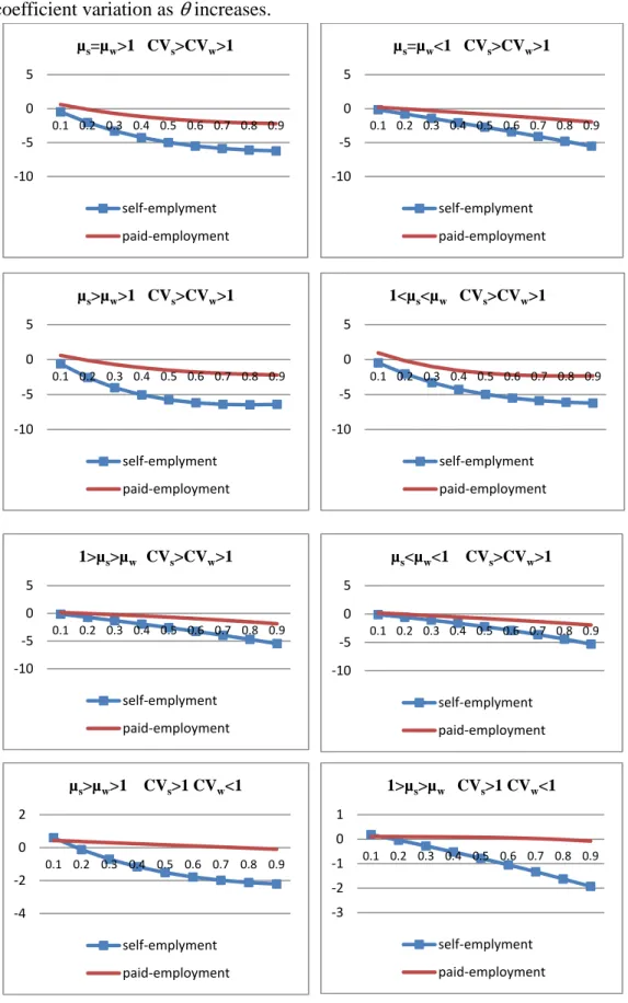
We are interested in assessing how increases in risk aversion affect the expected return from occupational choice at a fixed level of work effort. Figure 1 illustrates how expected utility from market work in each occupation changes as risk aversion increases. Graphs display various conditions on μy s, ,μy w, , CVs, and CVw. As
shown in Figure 1, as θ increases, expected utility from market work decreases in both self-employment and paid-employment. However, expected utility declines faster in self-employment than paid-employment and so paid employment becomes more attractive as θ increases. This evidence suggests that more risk averse agents who nevertheless choose employment will require a higher expected return from self-employment, and so μy s, must increase in θ. The reverse is true for the effect of θ on
expected earnings in paid employment: a more risk averse individual requires lower expected return than their less risk averse counterparts when they choose paid-employment. See the Appendix 1 for the proof.
Risk aversion has an ambiguous effect on work effort, whether in
self-employment (es) or wage work (ew). The reason is that effort depends on the utility from nonmarket work. Assuming 0 < e < 1, more risk averse individuals who receive high utility from nonmarket work or leisure will reduce work effort in the market production because increases in θ decrease utility from market work at any level of expected earnings. The reverse is true for those who have low utility from nonmarket work: more risk aversion increases market work effort in order to scale up the
We have shown that in reduced form, individual decisions on labor force participation, occupational choice, earnings, and work effort will depend on the individual’s degree of risk aversion as well as on predetermined skills in market and nonmarket production. Given the frequently reported finding that women are more risk averse than men, it is natural to presume that gender differences in risk preferences would play a role in explaining widely observed gender gaps in these labor market outcomes. Accordingly, this paper will examine the extent to which differences in measured risk aversion between men and women can explain differences between the sexes in labor force participation, entrepreneurial entry, earnings, and hours worked.
3. Empirical methodology and data 3.1 Methodology
To examine the influence of risk aversion on occupational choice, we employ a multinomial logit model using a random utility model approach. We run separate estimations for men and women for an appropriate comparison of the two groups. The predicted probability that an individual i chooses employment mode j is given by 3 1 1 I I 1 2 3 ij i i j i j i k i k i k Pr( C | , X ) exp(θ δ θ β X ) exp(δ θ β X ), j , , = ′ ′ = = +
∑
+ = (13)where j=1 for self-employment, 2 for paid-employment and 3 for out of labor force; the superscript I indicates an estimate of categorical risk attitude index; and θi is a
categorical variable indicating attitudes toward risk with higher levels indicating greater acceptance of risk. Our primary interest is in establishing the sign and significance of the coefficient on risk attitude, δjI. We also include a vector Xi that contains
presence of preschool or school age child (age 0~6, 7~12), marital status, education, labor market experience, health condition, parental education and occupational background, and other demographic variables such as age and four regions.
As an alternative specification, we replace θi by three dummy variables Dli, l =2, 3, 4; indicating progressively lower levels of risk aversion with unwillingness to take on any risk as the reference category (l =1). The associated predicted probability that individual i chooses employment mode j is given by
) exp( ) exp( ) , | 1 Pr( 3 1 4 2 4 2
∑
∑
∑
= = = ′ + ′ + = = k i k li l D lk i j l li D lj ij D X D X D X C δ β δ β (14)Next, we want to explore the extent to which differences in risk preferences explain differences in earnings and hours worked by gender. As men and women will be selecting hours and wages at the same time they are selecting occupation, those decisions will be subject to the same human capital and socio-demographic factors.
lnYikg =δ θ αkI i+ k′Zi+γ λ εk i+ ik ≡ Xiαk+εik (15)
lnhikg =δ θ αkI i+ k′Zi+γ λ εk i+ ik ≡ Xiψk +εik, k=s, w; g=m, f (16) where k=s for self-employment, w for paid-employment; g=m for male and f for female; vector Z contains the same variables as those in X except wealth and parental
occupational background. We only observe earnings and hours of work conditional on labor market entry, and so the earnings and labor supply equations also include a correction ( ) ( ) i k ik i k z z φ η λ η =
Φ for sample selection bias based on the procedure by
Heckman (1976, 1979). The zi augments vector Xi with risk aversion θi.
The data source for the analysis is drawn from the National Longitudinal Survey of Youth 79 (NLSY79) for the period between 1993 and 2002. The NLSY79 includes 12,686 individuals who were 14-22 years old in the initial survey year. 6,933
individuals aged between 28 and 45 were interviewed during the observation periods. Employment type is identified by using "class of worker" category, which indicates whether a respondent was employed by a private sector or government or was self-employed. We classify those who ever started a business in the period between 1994 and 2002 as self-employed. Hence, self-employment is identified using a 9-year longitudinal horizon to reflect long-term planning horizon that we presume applies to occupational choice. As a consequence, in our data, the decision to become self-employed is made between ages 29 and 45. Schiller and Crewson (1997) also
suggested that a longer life-cycle view for entrepreneurs would be preferred in the sense that new entrepreneurs may emerge in later years.
Those who never have a spell of self-employment but did work for pay were placed in the wage worker category over the 9 years time window. Respondents that did not report at least oneemployment spell over the period are considered out of the labor force.
Earnings are measured by the hourly pay rate. Although total annual earnings from wage and/or business in the previous calendar year can be identified in NLSY79, there are many missing values for self-employment earnings. Roughly 50 percent of the employed reported zero business earnings and about 11 percent of the self-employed with positive total annual earnings report zero income.2 This may be due to
2
NLSY79 asked respondents a question of “Did you receive earnings from business or farm in the past year?” In the following question, they were asked “what are total annual earnings from business or farm in the past calendar year?” In our data, 11% of respondents who answered ‘yes’ to the question over the observation years actually reported zero earnings.
self-employed reporting their income as wage or salary income (Fairlie, 2005). Because of the low response rate for the total annual business earnings, we incorporate earnings measured by hourly pay rate. For example, if a respondent identified himself as self-employed and reported hourly pay rate, we treat the self-reported hourly pay rate as self-employment hourly earnings. Because the observation time is between 1994 and 2002, we average their earnings over the years. Earnings are deflated by the CPI-U in 2002 dollars. Hours worked per week are also averaged over the years.
We drop those who were in military service or in school. We also drop individuals for whom critical information is missing. Finally, we exclude individuals who were already self-employed in 1993 to avoid reverse causal effects of experience of business ownership on risk attitudes. Therefore, the risk preference is measured before the spell of self-employment is initiated. The final sample includes 5,443 individuals; 2,662 males and 2,781 females.
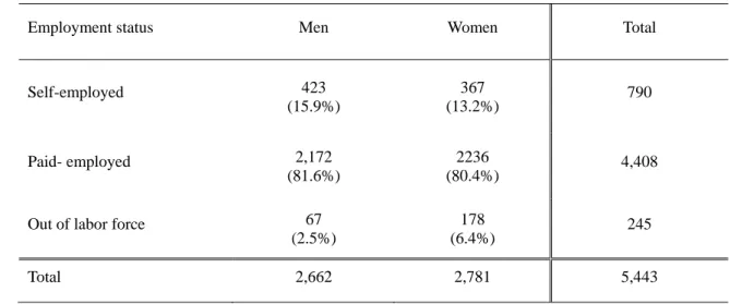
The distributions of employment type by gender over the period between 1994 and 2002 are summarized in Table 1. The longer time period eliminates most of the differences in labor force participation between men and women. Only 6 % of women and 3% of men were never employed over the 9 years. As shown, self-employment entry rate for women (13%) is lower than that for men (16%). Likewise, the
proportion of male wage workers (82%) is slightly larger than that for females (80%). A summary of self-employment rates, log hourly earnings and log hours worked across employment types by gender are reported in Table 2.3 Women earn less than men and they also work fewer hours than men regardless of employment type. These
differences in self-employment, earnings and labor supply between men and women are statistically significant, consistent with what has been found in the previous literature.
Definitions and descriptive statistics of the variables used in the analysis are reported separately by gender in Table 3.
3.3 Measures of risk attitudes
The willingness to take financial risk is measured by a categorical variable with four levels. In the 1993 NLSY79, respondents were asked the following questions:
(Q1) Suppose that you are the only income earner in the family, and you have a good job guaranteed to give you your current (family) income every year for life. You are given the opportunity to take a new and equally good job, with a 50-50 chance that it will double your (family) income and a 50-50 chance that it will cut your (family) income by a third. Would you take the new job?
The individuals who answered ‘yes’ to this question were then asked:
(Q2) suppose the chances were 50-50 that it would double your (family) income and 50-50 that it would cut it in half. Would you still take the new job? Those who answered ‘no’ to the first question (Q1) then asked: (Q3) suppose the changes were 50-50 that it would double your (family) income and 50-50 that it would cut it by 20 percent. Would you take the new job?
We use the responses to the series of questions in order to place each respondent into one of four risk categories (1-4). The four risk index categories, ranging from the most risk averse (category1) to the least risk averse (category4), are as followed:
1 2 3 4 riskindex ⎧ ⎪ ⎪ = ⎨ ⎪ ⎪⎩ if if if if Yes Q Yes Q No Q No Q = = = = 1 1 1 1 & & & & Yes Q No Q Yes Q No Q = = = = 2 2 3 3 ; ; ; ; accept accept reject reject cut cut cut cut 3 1 3 1 3 1 3 1 & & & & accept reject accept reject cut cut cut cut 2 1 2 1 5 1 5 1
In order to test for a monotonic relationship between a labor market outcome and degree of risk attitudes, we replace the risk attitude index with four dummy
variables to distinguish between levels of risk aversion: willingness to take 1) No risk; 2) Average risk; 3) Above average risk; 4) Substantial risk.
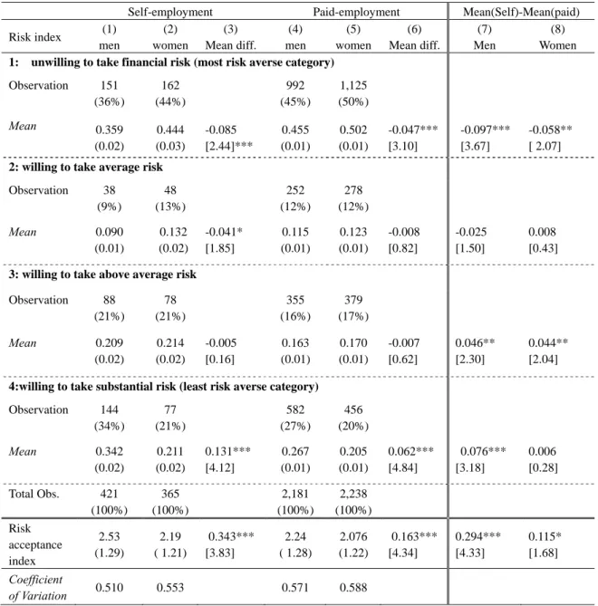
Past research has focused most on the role of risk aversion on entrepreneurship. The distribution of risk preferences across types of employment by gender is presented in Table 4. The first two columns show risk preferences for male and female
entrepreneurs. Surprisingly, both self-employed men and women are most commonly found in the most risk averse group: 36% of male and 44% of female entrepreneurs. However, the proportion of paid employees in the most risk averse category is even larger, consistent with the presumption that the most risk averse are more likely to select paid-employment over self-employment. Consistent with that supposition, 55% of male entrepreneurs are in the two least risk averse categories compared to only 43% of paid employees. Differences in risk preferences between female self-employed and paid-employed are less pronounced: 43% of female entrepreneurs and 37% of female paid employees are in the two least risk averse
groups. On the surface, it appears that risk preferences have a smaller effect on female entrepreneurial entry than it does on male entrepreneurship.
Columns (3) and (6) in Table 4 present two-sample t tests between men and women within occupation. Women are significantly more risk averse than men regardless of occupation. Columns (7) and (8) test for differences in risk aversion between the self-employed and the paid-employed. Entrepreneurs are less risk averse than are paid employees for both genders, but the differences are only marginally significant for women. Nor is the more modest gap in risk aversion between women self- and paid-employees due to less variation in risk preferences among women:
variation in risk preferences across women is comparable to the variation in risk preferences for men as shown in the final row of Table 4.
4. Empirical results
4.1 Effect of risk aversion on occupational choice by gender
In order to examine the influence of risk attitudes on occupational choice by gender, separate equations (13) and (14) were estimated for samples of men and women using a multinomial logit model. The estimated marginal effects are reported in Table 5 in two panels. In Panel A, risk preferences are measured by the four point risk attitude index that goes from most (1) to least (4) risk averse. In order to allow for a possible non- monotonic relationship between the probability of entry into self-employment and the degree of risk attitudes, we replace the risk attitude index with three dummy variables that indicate degree of willingness to take risk, considering willingness to take “no risk” as the reference category. Those estimates are reported in Panel B.
Turning first to the control measures, wealth increases the probability of moving into self-employment rather than being paid-employed for both men and women, consistent with the findings of previous studies (Evans and Leighton, 1989; Evans and Jovanovic, 1989; Blanchflower and Oswald, 1998; Fairlie, 2002). In line with Schiller and Crewson (1997), more employment experiences induce women to stay in paid employment and discourage them from transitioning into self-employment.
Conversely, men with more work experience are more likely to enter self-employment instead of paid-employment. Health limitations encourage men to work in their own
business. For women, those who reported health limitations tend to exit the labor force rather than enter the labor market.
Age, education and race have no significant effect on an employment choice regardless of gender. Lack of explanatory power of age might be because there are not enough variations in age in our sample. Having entrepreneurial or professional parents has no significant effect on the probability of becoming self-employment for both men and women.4
As shown in Table 5Panel A, more favorable attitudes toward risk raise the probability of being self-employed by 2.4 % and reduce the incidence of selecting paid-employment by 2.4% among men. The finding is as predicted in the theory and is also consistent with the previous literature on risk preferences (Kanbur 1979; Kihlstrom and Laffont 1979, Parker 1997; Van Praag and Cramer 2001; Hartog et al. 2002; Cramer et al. 2002; Ekelund et al. 2005; Kan and Tsai 2006; Ahn, T. 2009).5 However, there is no statistically significant effect of risk preferences on the probability that women enter either self-employment or paid-employment. Although the signs of the coefficients are the same as those for men, the magnitudes of the marginal effects for women are less than one-tenth those for men. Measured risk aversion does not affect the labor force participation decision for either men or women.
As the alternative specification shows in Panel B, for men, the marginal effects of the three risk attitude dummy variables on entry decision into self-employment are all positive and the size of the marginal effect gets progressively larger as willingness to take risk increases. For example, an individual who is willing to take above average
4
Manager, official and proprietor are in the same occupational category for parental occupational background in the NLSY79.
risk (substantial risk) has a 5.8% (7.6%) higher probability of being self-employed relative to the individual who is unwilling to take any risk. For women, on the other hand, the signs and magnitudes of the marginal effect of risk attitudes on
self-employment do not follow a systematic pattern and are never statistically significant. While risk attitudes play a key role in choosing entrepreneurship for men, they have no significant effect on women’s occupational choices.6
This finding suggests that men and women place different weights on future earnings in employment. Limited evidence on the motivations for entering self-employment may support this conjecture. For example, Georgellis and Wall (2005) found that larger expected earnings premia for self-employment versus
paid-employment increases entrepreneurial entry for men but not women. Clain (2000) showed that full-time self-employed women have characteristics that are less valued in the market compared to full-time paid-employed women. For men, the reverse is true, suggesting that women may place a higher value on non-pecuniary aspects of self-employment than do men.
4.2 Effect of risk aversion on hours and earnings by gender across
employment type
In this subsection, we examine the potential role of risk aversion on earnings and work hours by gender. As shown in section 2, a more risk averse agent requires higher expected earnings from self-employment whereas the more risk averse accepts lower expected earnings from paid-employment. The estimates of earnings model are
6
This study avoids a problem that the risk preferences is measure after the spell of self-employment is initiated by dropping those who were already self-employed when their risk attitudes were measured in 1993. Hartog et al. (2002) argue that ideally risk aversion should be measured before individuals make self-employment decision. Consequently, 402 observations were omitted from the sample. The results are, however, robust to including these individuals in the sample (See the Appendix 3).
reported in Panel A of Table 6. Consistent with the theory, greater risk aversion increases male returns to self-employment. However, there is no significant effect of measured risk preferences on the earnings of the female self-employed. The
coefficient on risk preferences for women is less than 98% of the size for men. This is consistent with our earlier finding that risk aversion does not affect women’s entry decision on self-employment.
For men engaged in wage work, willingness to accept risk is associated with lower male wage which is inconsistent with theory. The most risk averse are paid almost 12% more than the least risk averse. The least risk averse women are paid more in wage work consistent with the theory, although the differences are small. Going from the least to the most risk averse lowers pay by 6%.7
Risk aversion can also affect hours of labor supplied although the direction of the effect is ambiguous. We estimated equation (16) and report the estimated risk aversion effect by gender and employment type in Panel B of Table 6. The complete results from the labor supply estimation are presented in Appendix 5. As with our labor force participation results, there is no significant relationship between risk preferences and hours of work for either men or women.
4.3 Do gender differences in risk aversion explain the observed gender gaps in
the labor market outcomes?
Given our behavioral estimates of the entrepreneurial choice, earnings, and hours of labor supply decisions, we can now assess the extent to which gender
differences in risk aversion explain the gender gaps in these labor market outcomes.
7
Estimates of log annual earnings are reported in Appendix 4. The signs on risk preferences are consistent with those from log hourly earnings although the estimates lose precision.
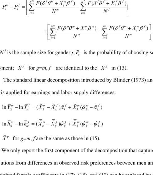
To measure how much differences in risk preferences between men and women explain the gender gap in entrepreneurial choice, we apply Fairlie’s (1999) nonlinear variant of the Blinder-Oaxaca decomposition. The difference in probability of self-employment across genders is
1 1 ( ) ( ) m f m m f f f f f f N N m f i i s s m f i i F X F X P P N N δ θ β δ θ β = = ⎡ + + ⎤ − =⎢ − ⎥ ⎣
∑
∑
⎦ 1 1 ( ) ( ) m m m m m f f m m f N N i i m m i i F X F X N N δ θ β δ θ β = = ⎡ + + ⎤ +⎢ − ⎥ ⎣∑
∑
⎦ (17)where Nj is the sample size for gender j;Ps is the probability of choosing self-employment; Xg for g=m, f are identical to the Xg in (13).
The standard linear decomposition introduced by Blinder (1973) and Oaxaca (1973) is applied for earnings and labor supply differences:
ˆ ˆ ˆ
lnYikm −lnYikf =(Xkm −Xkf)αkf +Xkm(αkm−αkf) (18)
ˆ ˆ ˆ
lnhikm−lnhikf =(Xkm −Xkf)ψkf +Xkm(ψkm−ψkf) (19) where Xg for g=m, f are the same as those in (15).
We only report the first component of the decomposition that captures
contributions from differences in observed risk preferences between men and women. The weighted female coefficients in (17), (18), and (19) can be replaced by male’s estimates or pooled estimates.
Table 7 reports percentage contribution of risk preferences to the gender gaps in three outcomes by employment type. The percentage contribution is calculated as estimated coefficient from decomposition dividing by mean difference in outcome (i.e., entrepreneurial choice, earnings, or hours of work) and then multiplying by 100. The
female coefficients from table 6 are used in specification 1 and the male coefficients are applied in specification 2. Estimates for a pooled sample of men and women are incorporated in specification 3.
Conclusions based on the decomposition analysis are sensitive to the choice of coefficient on self-employment.8 For instance, gender differences in risk aversion explain 2% of the entrepreneurial choice gap between men and women in the female-weighted decomposition, but 12 % of the gap in the male-female-weighted decomposition. Similarly, if women had risk preferences equal to those of men, their entrepreneurial earnings would be only about 1% less if we take women’s coefficients as weights, but would be 19% lower using men’s coefficients. Regardless of choice of coefficients applied, risk preferences explain little of the difference in hours worked or earnings from wage work between men and women.
Most commonly, researchers use the male coefficients in decompositions
because of a presumption that the male coefficients are not subject to discrimination. However, this application reflects behavioral decisions regarding occupation, earnings and hours worked. Therefore, it is appropriate to see how a woman with risk
preferences equivalent to those of a male would have affected her behavioral decisions regarding choice of occupation and associated occupational earnings and hours of work. That argument suggests that we should use the female-weighted decomposition to
analyze how much risk preferences would affect female labor market outcomes.9 Using that criterion, risk preferences explain only 1.9% of the gap in
entrepreneurial choice between men and women. Equalizing risk preferences across
8
This is a common problem so called “index number problem” in the standard decomposition. See Oaxaca (1973) for more detail.
9
For a linear case, (θm−θ δf)ˆf =θ δmˆf −θ δf ˆf. The first term is counterfactual earnings that women would have if women had men’s risk aversion level. The second term is actual earnings. Expected change in women’s entrepreneurial choice can be measured as the same way.
the genders would alter relative women’s pay by only about 1% in either self-employment or paid self-employment. Likewise, equalizing risk preferences would change relative women’s hours worked by less than 1% in both occupations.
4.4 Sensitivity Analysis
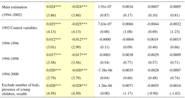
The aim of this subsection is to show the extent to which conclusions regarding the impact of risk preferences on labor market choices are robust to changes in
specification. The first change is to replace all individual attributes that were averaged over the 9 year estimation window with their start-of-period (i.e., 1993) values.
Second, different time spans for observing labor market outcomes are used: 1994-1996, 1994-1998 and 1994-2000. Finally, potentially endogenous variables such as number of children, presence of young children and wealth are excluded as control variables from the estimation. The estimated marginal effects of risk attitudes are presented in Table 8. The main estimation results are reported in the first row for reference. In all instances, we find that increasing willingness to accept risk raises the probability of self-employment and lowers the probability of wage work only for men. In all specifications, risk preferences do not affect women’s occupational choices.
We use the same modifications to our specifications to evaluate the robustness of our results for earnings and labor supply. The results reported in Table 9 show that the signs on risk preferences are stable in most cases. When signs are not consistent with the main estimates the significance level falls below 10%.
Table 10 reports contributions of risk preferences to the gender gap in entrepreneurial choice, earnings, and hours of labor supply. We only focus on the specification 1 (female-weighted decomposition) and so we are assessing how women’s estimated behavioral choices would have been different had they had the risk
preferences of an average male in the population. Depending on specification, differences in risk preferences explain only 0.1% to 4.5% of the gap in entrepreneurial choice between men and women. With one exception, the entrepreneurial earnings gap would be even larger if women had the same level of risk acceptance as men. The gender pay gap for wage work and for hours worked are also largely unaffected by differences in risk preferences between men and women with the explained gap rarely exceeding 1% in absolute value. In short, the commonly observed differences in risk preferences across genders explain little of the observed gaps in labor market outcomes between men and women.
5. Summary and conclusion
This study examines the extent to which gender differences in risk preferences can explain male-female gaps in self-employment rate, earnings, and labor supply. Exploiting a 9-year longitudinal sample of men and women in the NLSY79, we confirm the standardized gender gap reported in the previous literature: on average, women are less likely to become self-employed, earn less and work fewer hours than men. Furthermore, NLSY79 shows that considerable differences in measured risk
preferences between men and women exist: women are more risk averse than men. In a theoretical framework, we show the potential role of risk aversion in occupational choice, earnings, and hours of work: negative relationship between risk aversion and entrepreneurial choice, positive relationship between risk aversion and expected return from self-employment, and negative relationship between risk aversion and expected wage from paid-employment. Although risk aversion can also affect hours of work, the direction of effect cannot be signed.
We find that risk preferences are an important factor that affects occupational choice for men – less risk averse men tend to become self-employed and more risk averse men become wage workers. However, there is no relationship between degree of risk preferences and occupational choice for women. A different role of risk preferences in earnings by gender across employment type is also found. Less risk aversion is associated with lower male earnings in self-employment. On the other hand, there is no significant effect of measured risk preferences on female
entrepreneurial earnings. In paid-employment, less risk aversion lowers the male wage whereas it raises female wages. Finally, we find no relationship between risk aversion and hours of labor for both men and women across employment type.
Consequently, the Blinder-Oaxaca decomposition shows that gender differences in risk attitudes explain only small part of gender gap in self-employment rate.
Similarly, those differences in risk preferences account for only a trivial portion of the gender gap in hours worked or earnings. The results hold up well against a variety of sensitivity checks. These findings suggest that widely reported differences in risk preferences across genders do not play a role in explaining differences in labor market outcomes between men and women.
References
Ahn, T. (2009) Attitudes toward risk and self-employment of young workers, Labour
Economics, 17, 434-442.
Barsky, R.B., Juster, F.T., Kimball, M.S., and Shapiro, M.D. (1997) Preference
parameters and behavioral heterogeneity: An experimental approach in the health and retirement study, The Quarterly Journal of Economics, 112, 537-579.
Blanchflower, D. G. and Oswald, A. J. (1998) What makes an entrepreneur? Journal of
Labor Economics, 16, 26–60.
Blinder, A. (1973) Wage discrimination: Reduced form and structural estimates,
Journal of Human Resources, 8, 436-455.
Boden, R.J. (1999) Flexible working hours, family responsibilities, and female self-employment, American Journal of Economics and Sociology, 58, 71-83. Borghans, L., Golsteyn, B.H., Heckman, J.J., and Meijers, H. (2009) Gender
differences in risk aversion and ambiguity aversion, The Institute for the Study of Labor (IZA), Discussion Paper No. 3985
Bonin, H., Dohmen, T., Falk, A., Huffman, D., and Sunde, U. (2007) Cross-sectional earnings risk and occupational sorting: The role of risk attitudes, Labour
Economics, 14, 926–937
Croson, R. and Gneezy, U. (2009) Gender differences in preferences. Journal of
Economic Literature, 47(2), 1–27.
Clain, S. H. (2000) Gender differences in full-time self-employment, Journal of
Economics and Business, 52, 499–513.
Connelly, R. (1992) Self-employment and providing child care, Demography, 29, 17-29.
Cramer, J.S., Hartog, J., Jonker, N., and Van Praag, C.M. (2002) Low risk aversion encourages the choice for entrepreneurship: an empirical test of a truism, Journal
Dunn, T. and Holtz-Eakin, D. (2000) Financial capital, human capital, and the transition to self-employment: evidence from intergenerational links, Journal of Labour
Economics, 18, 282–305.
Eckel, C. C. and Grossman, P. J. (1998) Are women less selfish than men? Evidence from dictator experiments. Economic Journal, 108 (448), 726–735.
Ekelud, J., Johansson, E., Jarvelin M-R, and Lichtermann, D. (2005) Self-employment and risk aversion-evidence from psychological test data, Labour Economics, 12, 649-659.
Evans, D. S. and Jovanovic, B. (1989) An estimated model of entrepreneurial choice under liquidity constraints, Journal of Political Economy, 97, pp. 808–827. Evans, D. S. and Leighton, L. S. (1989) Some empirical aspects of entrepreneurship,
American Economic Review, 79, 519–535.
Fairlie, R.W. (1999) The Absence of the African-American Owned Business: An Analysis of the Dynamics of Self-Employment, Journal of Labor Economics, 17(1), 80-108.
Fairlie, R.W. (2002) Drug dealing and legitimate self-employment, Journal of Labor
Economics, 20, 538-567.
Fairlie, R.W. (2005) Self-employment, entrepreneurship, and the NLSY79, Monthly
Labor Review, February, 40-47.
Georgellis, Y. and Wall, H. (2005) Gender differences in self-employment,
International review of applied economics, 19, 321-342.
Gneezy, U., Niederle, M., and Rustichini, A. (2003) Performance in competitive environments: Gender Differences, Quarterly Journal of Economics, 118(3), 1049-1074.
Hansen, L.P., and Singleton, K.J. (1983) Stochastic Consumption, Risk Aversion, and the Temporal Behavior of Asset Returns, Journal of Political Economy, 91(2), 249-265.
Hartog, J., Ferrer-i-Carbonell, A., and Jonker, N. (2002) Linking measured risk aversion to individual characteristics, Kyklos, 55, 3-26.
Heckman, J.J. (1976) The Common Structure of Statistical Models of Truncation, Sample Selection and Limited Dependent Variables and a Simple Estimator for Such Models, Analysis of Economic Social Management, 5(4), 475-492. Heckman, J.J. (1979) Sample Selection Bias as a Specification Error, Econometrica,
47(1), 53-161.
Holtz-Eakin, D., Joulfaian, D. and Rosen, H. S. (1994) Entrepreneurial decisions and liquidity constraints, Rand Journal of Economics, 25, 334–347.
Hout, M. and Rosen, H. S. (2000) Self-employment, family background, and race,
Journal of Human Resources, 35, 670–692.
Hundley, G. (2000). Male/female earnings differences in self-employment: the effects of marriage, children, and the household division of labour, Industrial and Labour
Relations Review, 54, 95–115.
Johnson, W. (1978) A theory of job-shopping, Quarterly Journal of Economics, 22, 261-278.
Kanbur, S.M. (1979). Of Risk taking and the personal, distribution of income. Journal
of Political Economy, 87, 760-97.
Kan, K. and Tsai, W. (2006) Entrepreneurship and risk aversion, Small business
economics, 26, 465-474.
Kaplow, Louis (2005) The Value of a Statistical Life and the Coefficient of Relative Risk Aversion, The Journal of Risk and Uncertainty, 31(1), 23–34.
Kihlstrom, R.E. and Laffont, J.J. (1979). A general equilibrium entrepreneurial theory of new firm formation based on risk aversion. Journal of Political Economy, 87, 304-16.
Kimball, M.S., Sahm, C.R. and Shapiro, M.D. (2008) Imputing risk tolerance from survey responses, American Statistical Association, 103, 1028-1038.
Knight, F.H. (1921). Risk, Uncertainty and Profit. Houghton Mifflin, New York. Le, A., Miller, P., Slutske, W., and Martin, N. (2010) Attitudes towards Economic Risk
and the Gender Pay Gap, IZA DP No. 5393.
Lentz B.F. and Laband D.N. (1990) Entrepreneurial success and occupational
inheritance among proprietors, Canadian Economics Association, 23, 101-117. Maddala, G.S. (1983) Limited dependent and qualitative variables in econometrics,
Econometric Society Monographs in Quantitative economics No. 3, Cambridge University Press.
Miller, R. (1984) Job matching and occupational choice, Journal of Political Economy, 92, 1086-120.
Mueller, Gerrit and Erik Plug. 2006. “Estimating the Effect of Personality on Male and Female Earnings.” Industrial and Labor Relations Review 60 (October): 3-22. Newbery, D.M.G. and Stiglitz, J. (1982) Risk Aversion, Supply Response and the
Optimality of Random Prices: A Diagrammatical Analysis.Quarterly Journal of
Economics, 97, 1-26.
Niederle, M. and Vesterlund, L. (2007) Do Women Shy Away from Competition? Do Men Compete too Much? Quarterly Journal of Economics, 122(3), 1067-1101. Oaxaca, R.L. (1973) Male-Female wage differentials in urban labor markets,
International Economic Review, 14, 693-709.
Parker, S.C. (1997) The effects of risk on self-employment, Small business economics, 9, 515-522.
Pålsson, Anne-Marie (1996) Does the Degree of Relative Risk Aversion Vary with Household Characteristics?, Journal of Economic Psychology 17, 771–787. Pratt, J. (1964). Risk aversion in the small and in the large. Econometrica, 32, 122–136. Schiller, B. and Crewson, P. (1997) Entrepreneurial origins: a longitudinal inquiry,
Strohmeyer, R. (2003) Gender differences in self-employment: does education matter? Paper presented at the ICSB, 48th World Conference, Belfast.
Tucker, I.B. (1988) Entrepreneurs and public-sector employees: the role of achievement motivation and risk in occupational choice, Journal of Economic Education, 19, 259-268.
Taylor, M. P. (1996) Earnings, independence, or unemployment: why become self-employed?, Oxford Bulletin of Economics and Statistics, 58, 253–266.
Van Praag, C.M. and Cramer, J.S. (2001) The roots of entrepreneurship and labour demand: Individual ability and low risk aversion, Economica, 2001, 45-62.
Figure 1 Change in expected utility associated with various expected return and coefficient variation as θ increases.
‐10 ‐5 0 5 0.1 0.2 0.3 0.4 0.5 0.6 0.7 0.8 0.9 µs=µw>1 CVs>CVw>1 self‐emplyment paid‐employment ‐10 ‐5 0 5 0.1 0.2 0.3 0.4 0.5 0.6 0.7 0.8 0.9 µs=µw<1 CVs>CVw>1 self‐emplyment paid‐employment ‐10 ‐5 0 5 0.1 0.2 0.3 0.4 0.5 0.6 0.7 0.8 0.9 µs>µw>1 CVs>CVw>1 self‐emplyment paid‐employment ‐10 ‐5 0 5 0.1 0.2 0.3 0.4 0.5 0.6 0.7 0.8 0.9 1<µs<µw CVs>CVw>1 self‐emplyment paid‐employment ‐10 ‐5 0 5 0.1 0.2 0.3 0.4 0.5 0.6 0.7 0.8 0.9 1>µs>µw CVs>CVw>1 self‐emplyment paid‐employment ‐10 ‐5 0 5 0.1 0.2 0.3 0.4 0.5 0.6 0.7 0.8 0.9 µs<µw<1 CVs>CVw>1 self‐emplyment paid‐employment ‐4 ‐2 0 2 0.1 0.2 0.3 0.4 0.5 0.6 0.7 0.8 0.9 µs>µw>1 CVs>1 CVw<1 self‐emplyment paid‐employment ‐3 ‐2 ‐1 0 1 0.1 0.2 0.3 0.4 0.5 0.6 0.7 0.8 0.9 1>µs>µw CVs>1 CVw<1 self‐emplyment paid‐employment
Note: CVs and CVw denote coefficient variation in self-employment and paid-employment, respectively.
The case of CVw<CVs<1 is not considered because if both CVs and CVw are less than 1, there is little
difference in risk between s and w.
‐4 ‐2 0 2 0.1 0.2 0.3 0.4 0.5 0.6 0.7 0.8 0.9 1<µs<µw CVs>1 CVw<1 self‐emplyment paid‐employment ‐2 ‐1 0 1 0.1 0.2 0.3 0.4 0.5 0.6 0.7 0.8 0.9 µs<µw<1 CVs>1 CVw<1 self‐emplyment paid‐employment
Table 1 Distribution of employment status (1994~2002) by gender aged 29~45
Employment status Men Women Total
Self-employed 423 (15.9%) 367 (13.2%) 790 Paid- employed 2,172 (81.6%) 2236 (80.4%) 4,408
Out of labor force 67
(2.5%)
178
(6.4%) 245
Table 2 Self-employment rate, hourly earnings and labor supply by gender
Mean (std)
(1) Men (2) Women (3) Mean Differences Self-employment Self-employment rate 0.16
(0.01)
0.13 (0.01)
0.03*** (2.82)
Log hourly earnings 7.20
(0.93) 6.80 (1.05) 0.39*** (0.07) Obs. 397 328
Log hours worked 3.88
(0.38) 3.51 (0.68) 0.36*** (0.04) Obs. 364 307
Paid-employment Log hourly earnings 7.53 (0.59) 7.22 (0.59) 0.31*** (0.02) Obs. 2,159 2,216
Log hours worked 3.80
(0.00) 3.60 (0.01) 0.20*** (0.01) Obs. 2,148 2,171
Table 3 Definitions and descriptive statistics of variables
Definition
Men Women
Mean (Std) Mean (Std)
Risk acceptance index (1-4) Four point risk attitude index: increasing in
willingness to take financial risk
2.29 (1.28) 2.09(1.22)
Willingness to take:
No risk =1 if risk index=1 0.44 (0.50) 0.50 (0.50)
Average risk =1 if risk index=2 0.11 (0.31) 0.13 (0.33)
Above average risk =1 if risk index=3 0.17 (0.38) 0.17 (0.38)
Substantial risk =1 if risk index=4 0.28 (0.45) 0.21 (0.41)
log(net-asset) Difference between all asset values and all debts 14.23 (0.33) 14.21 (0.45)
Education Years of schooling completed 12.81 (2.41) 12.84 (2.36)
Work experience (in year) Years of employment experience 14.67 (4.09) 11.97(5.38)
Number of kids Number of bio/step/adopted children in HH 1.17 (1.15) 1.67(1.17)
Presence of pre-school kid =1 if pre-school age child (age<6) is present 0.32 (0.33) 0.35 (0.34)
Presence of school kid =1 if a child aged 7 to 12 is present 0.16 (0.21) 0.26 (0.22)
Age Age in years 35.69 (2.28) 35.81(2.23)
Married, spouse present =1 if married and spouse present 0.56 (0.43) 0.55 (0.44)
Health limitation =1 if health problem limits ability to work 0.08 (0.21) 0.12(0.24)
White =1 if white 0.64 (0.48) 0.63(0.48)
Father education Years of schooling his/her father completed 10.70 (4.22) 10.48 (4.15)
Father professional/proprietor =1 if father has/had professional/proprietor 0.10 (0.29) 0.09 (0.29)
Mother education Years of schooling his/her mother completed 10.81 (3.27) 10.63 (3.13)
Mother professional/proprietor =1 if mother has/had professional/proprietor 0.03 (0.16) 0.02(0.14)
Urban =1 if reside in urban area 0.76 (0.34) 0.76 (0.34)
Northeast =1 if reside in northeast 0.34 (0.36) 0.16 (0.36)
North central =1 if reside in north central 0.24 (0.42) 0.23 (0.42)
South =1 if reside in south 0.41 (0.48) 0.42(0.48)
Table 4 Measured risk preferences by occupational choice and gender
Note: Column (3), (6) are two-sample t test between men and women within self-employment and paid-employment, respectively. Column (7), (8) are two-sample t test between self- and paid-employment within gender and risk aversion. ***/**/* indicates significance at the 1%/5%/10% level. Standard errors are in parenthesis. t-statistics are in bracket.
Self-employment Paid-employment Mean(Self)-Mean(paid)
Risk index (1) men (2) women (3) Mean diff. (4) men (5) women (6) Mean diff. (7) Men (8) Women
1: unwilling to take financial risk (most risk averse category)
Observation 151 (36%) 162 (44%) 992 (45%) 1,125 (50%) Mean 0.359 (0.02) 0.444 (0.03) -0.085 [2.44]*** 0.455 (0.01) 0.502 (0.01) -0.047*** [3.10] -0.097*** [3.67] -0.058** [ 2.07]
2: willing to take average risk
Observation 38 (9%) 48 (13%) 252 (12%) 278 (12%) Mean 0.090 (0.01) 0.132 (0.02) -0.041* [1.85] 0.115 (0.01) 0.123 (0.01) -0.008 [0.82] -0.025 [1.50] 0.008 [0.43]
3: willing to take above average risk
Observation 88 (21%) 78 (21%) 355 (16%) 379 (17%) Mean 0.209 (0.02) 0.214 (0.02) -0.005 [0.16] 0.163 (0.01) 0.170 (0.01) -0.007 [0.62] 0.046** [2.30] 0.044** [2.04]
4:willing to take substantial risk (least risk averse category)
Observation 144 (34%) 77 (21%) 582 (27%) 456 (20%) Mean 0.342 (0.02) 0.211 (0.02) 0.131*** [4.12] 0.267 (0.01) 0.205 (0.01) 0.062*** [4.84] 0.076*** [3.18] 0.006 [0.28] Total Obs. 421 (100%) 365 (100%) 2,181 (100%) 2,238 (100%) Risk acceptance index 2.53 (1.29) 2.19 ( 1.21) 0.343*** [3.83] 2.24 ( 1.28) 2.076 (1.22) 0.163*** [4.34] 0.294*** [4.33] 0.115* [1.68] Coefficient of Variation 0.510 0.553 0.571 0.588
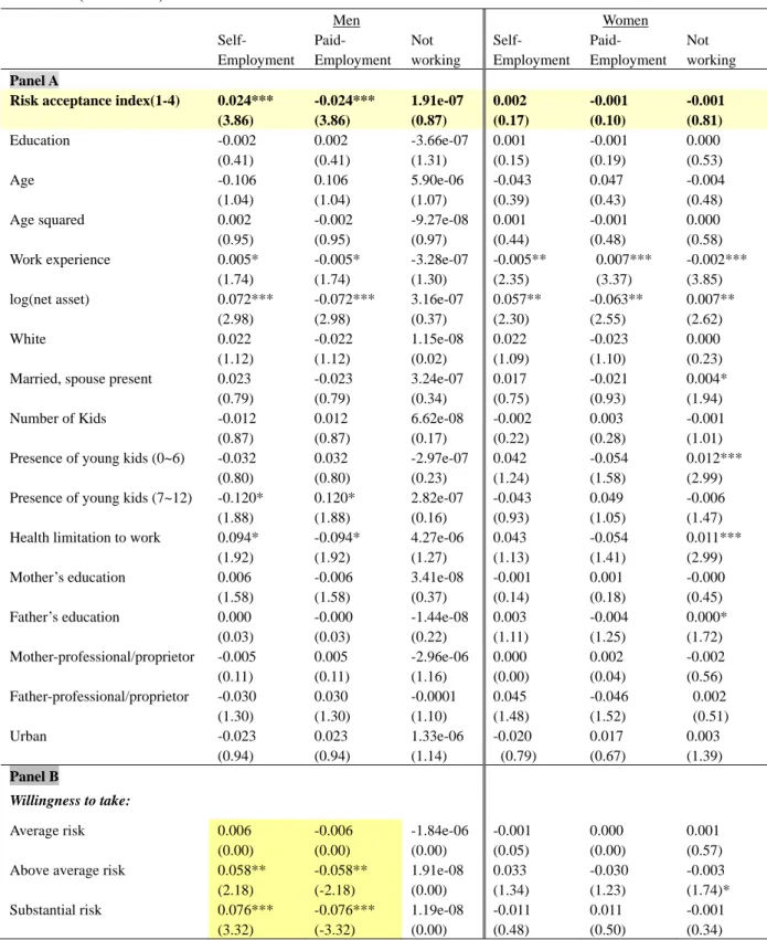
Table 5 Multinomial Logit Marginal Effects of Determinants of Occupational Choice for Men and Women (1994~2002) Men Women Self- Employment Paid-Employment Not working Self-Employment Paid-Employment Not working Panel A
Risk acceptance index(1-4) 0.024***
(3.86) -0.024*** (3.86) 1.91e-07 (0.87) 0.002 (0.17) -0.001 (0.10) -0.001 (0.81) Education -0.002 (0.41) 0.002 (0.41) -3.66e-07 (1.31) 0.001 (0.15) -0.001 (0.19) 0.000 (0.53) Age -0.106 (1.04) 0.106 (1.04) 5.90e-06 (1.07) -0.043 (0.39) 0.047 (0.43) -0.004 (0.48) Age squared 0.002 (0.95) -0.002 (0.95) -9.27e-08 (0.97) 0.001 (0.44) -0.001 (0.48) 0.000 (0.58) Work experience 0.005* (1.74) -0.005* (1.74) -3.28e-07 (1.30) -0.005** (2.35) 0.007*** (3.37) -0.002*** (3.85) log(net asset) 0.072*** (2.98) -0.072*** (2.98) 3.16e-07 (0.37) 0.057** (2.30) -0.063** (2.55) 0.007** (2.62) White 0.022 (1.12) -0.022 (1.12) 1.15e-08 (0.02) 0.022 (1.09) -0.023 (1.10) 0.000 (0.23) Married, spouse present 0.023
(0.79) -0.023 (0.79) 3.24e-07 (0.34) 0.017 (0.75) -0.021 (0.93) 0.004* (1.94) Number of Kids -0.012 (0.87) 0.012 (0.87) 6.62e-08 (0.17) -0.002 (0.22) 0.003 (0.28) -0.001 (1.01) Presence of young kids (0~6) -0.032
(0.80) 0.032 (0.80) -2.97e-07 (0.23) 0.042 (1.24) -0.054 (1.58) 0.012*** (2.99) Presence of young kids (7~12) -0.120*
(1.88) 0.120* (1.88) 2.82e-07 (0.16) -0.043 (0.93) 0.049 (1.05) -0.006 (1.47) Health limitation to work 0.094*
(1.92) -0.094* (1.92) 4.27e-06 (1.27) 0.043 (1.13) -0.054 (1.41) 0.011*** (2.99) Mother’s education 0.006 (1.58) -0.006 (1.58) 3.41e-08 (0.37) -0.001 (0.14) 0.001 (0.18) -0.000 (0.45) Father’s education 0.000 (0.03) -0.000 (0.03) -1.44e-08 (0.22) 0.003 (1.11) -0.004 (1.25) 0.000* (1.72) Mother-professional/proprietor -0.005 (0.11) 0.005 (0.11) -2.96e-06 (1.16) 0.000 (0.00) 0.002 (0.04) -0.002 (0.56) Father-professional/proprietor -0.030 (1.30) 0.030 (1.30) -0.0001 (1.10) 0.045 (1.48) -0.046 (1.52) 0.002 (0.51) Urban -0.023 (0.94) 0.023 (0.94) 1.33e-06 (1.14) -0.020 (0.79) 0.017 (0.67) 0.003 (1.39) Panel B Willingness to take: Average risk 0.006 (0.00) -0.006 (0.00) -1.84e-06 (0.00) -0.001 (0.05) 0.000 (0.00) 0.001 (0.57)
Above average risk 0.058**
(2.18) -0.058** (-2.18) 1.91e-08 (0.00) 0.033 (1.34) -0.030 (1.23) -0.003 (1.74)* Substantial risk 0.076*** (3.32) -0.076*** (-3.32) 1.19e-08 (0.00) -0.011 (0.48) 0.011 (0.50) -0.001 (0.34) Note: 1) The reference category in Panel B is willingness to take “no risk”. 2) Same control variables as Panel A are included in Panel B and C. 3) 4 regions are also included in all Panels) 4) Standard errors can be provided on request 4)***/**/* indicates significance at the 1%/5%/10% level.
Table 6 Estimates of Earnings and labor supply for self-employed, paid-employed and overall labor force participants by gender
Self-employment Paid-employment
Male Female Male Female
Panel A log hourly earnings
Risk acceptance index -0.192***
(3.54) -0.004 (0.08) -0.039*** (3.20) 0.020** (2.12) Education 0.081*** (3.48) 0.021 (0.59) 0.085*** (14.75) 0.080*** (13.28) Age 0.889 (1.27) -0.632 (0.74) -0.238 (1.61) -0.123 (0.78) Age squared -0.013 (1.16) 0.009 (0.68) 0.004* (1.66) 0.001 (0.60) Work experience -0.031 (1.47) 0.043** (2.54) 0.031*** (7.83) 0.049*** (9.49) White -0.014 (0.11) -0.189 (0.99) 0.053* (1.79) -0.013 (0.43) Married 0.051 (0.30) -0.501** (2.61) 0.000 (0.01) -0.074** (2.28) Number of kids -0.010 (0.12) -0.038 (0.44) 0.028 (1.58) 0.013 (0.80)
Presence of a kid aged under 6 0.152 (0.61) -0.497* (1.68) 0.140** (2.45) -0.111** (2.14)
Presence of a kid aged 7-12 1.120*** (2.99) 0.077 (0.21) 0.251*** (2.96) 0.049 (0.71) Health problem -0.788** (2.52) -0.620* (1.85) -1.091*** (7.92) -0.283*** (4.12) Mother education -0.066*** (3.19) -0.016 (0.57) 0.002 (0.39) 0.001 (0.22) Father education 0.027* (1.68) 0.005 (0.25) 0.004 (1.04) 0.001 (0.34) Urban 0.207 (1.29) 0.268 (1.23) 0.107*** (2.98) 0.131*** (3.63) Years in business 0.121*** (3.19) 0.159** (2.53) - - Heckman’s selection -9.032*** (3.94) -13.100*** (3.07) 4.731*** (6.06) 1.097* (1.85) R2 0.2327 0.2025 0.3403 0.3611 N 309 242 1651 1530
Panel B log hours of labor
Risk attitudes -0.030 (1.36) -0.003 (0.08) -0.004 (0.90) -0.002 (0.36) R2 0.153 0.201 0.059 0.223 N 277 221 1629 1488
Note: Risk acceptance index is measured by a categorical variable from the most (1) to the least risk averse. In Panel A, average hourly earnings are dependent variable. In Panel B, average hours worked per week are dependent variable. Same controls in Panel A are used in Panel B. Four regions are controlled in both Panels. t-statistics are in parentheses. */**/*** refer significance levels of 10%, 5%, and 1%. The complete results from the labor supply estimation are presented in Appendix 5.
Table 7 Decomposition for occupational choice, earnings and labor supply models: estimates of percentage of gender gap due to Male/Female differences in Risk preferences
(1) Female coefficient (2) Male coefficient (3) Pooled coefficient Entrepreneurial choice Coefficient 0.0004 0.0024 0.0018 Difference 0.0202 0.0202 0.02022 Percentage 1.9% 11.8% 8.8% Log Earnings Self-employed Coefficient -0.0022 -0.0835 -0.0120 Difference 0.4366 0.4366 0.4366 Percentage -0.5% -19.1% -2.7% Paid-employed Coefficient 0.0028 -0.0052 0.0021 Difference 0.3121 0.3121 0.3121 Percentage 0.9% -1.7% 0.7%
Log hours worked
Self-employed Coefficient -0.0012 -0.0130 0.0031 Difference 0.4162 0.4162 0.4162 Percentage -0.3% -3.1% 0.8% Paid-employed Coefficient -0.0003 -0.0006 0.0014 Difference 0.2037 0.2037 0.2037 Percentage -0.1% -0.3% 0.7%
Note) Difference indicates mean differences in outcomes such as entrepreneurial choice, earnings, and hours of labor. Percentage is calculated as (coefficient/difference)*100.
Table 8 Robustness of risk preferences in occupational choice
Men (four point risk index) Women (four point risk index)
Self-Employment Paid-Employment Not working Self Employment Paid-Employment Not working Main estimation (1994~2002) 0.024*** (3.86) -0.024*** (3.86) 1.91e-07 (0.87) 0.0016 (0.17) -0.0007 (0.10) -0.0005 (0.81) 1993 Control variables 0.025*** (4.13) -0.025*** (4.13) 7.63e-07 (0.00) 0.0066 (1.08) -0.0044 (0.69) -0.0022 (1.23) 1994-1996 0.012*** (3.01) -0.012*** (2.99) -0.0000 (0.11) -0.0004 (0.09) 0.0019 (0.40) -0.0015 (0.66) 1994-1998 0.017*** (3.58) -0.017*** (3.56) -0.0001 (0.54) 0.0038 (0.77) -0.0029 (0.57) -0.0009 (0.71) 1994-2000 0.020*** (3.79) -0.020*** (3.79) -7.38e-06 (0.04) 0.0035 (0.60) -0.0028 (0.48) -0.0007 (0.74) Exclude number of kids,
presence of young children, wealth 0.028*** (4.59) -0.028*** (4.50) 1.26e-06 (0.00) 0.0071 (1.17) -0.0055 (-0.90) -0.0016 (-1.62) Note: 1) t-statistics are reported in parenthesis. 2) ***/**/* indicates significance at the 1%/5%/10% level.
Table 9 Robustness of risk preferences in earnings and labor supply
Self-employment Paid-employment
Male Female Male Female
Panel Alog hourly earnings
Main estimate (1994-2002) -0.192*** (3.54) -0.004 (0.08) -0.039*** (3.20) 0.020** (2.12) 1993 Control variables -0.143** (2.42) 0.033 (0.54) -0.041*** (2.67) 0.020** (2.16) 1994-1996 -0.103 (1.26) -0.095 (1.21) 0.021 (1.46) -0.011 (0.62) 1994-1998 -0.176* (1.90) -0.103 (1.03) 0.021 (1.07) 0.007 (0.30) 1994-2000 -0.196 (1.28) -0.100 (0.73) 0.036 (1.36) 0.048 (1.52)
Exclude number of kids, presence of
young children, wealth
-0.140*** (2.73) -0.004 (0.08) -0.014 (1.25) 0.019** (2.01)
Panel Blog hours worked
Main estimate (1994-2002) -0.030 (1.36) -0.003 (0.08) -0.004 (0.90) -0.002 (0.36) 1993 Control variables -0.056** (2.25) -0.011 (0.26) -0.005 (1.19) 0.001 (0.20) 1994-1996 -0.146* (1.76) -0.031 (0.25) -0.014 (1.01) -0.018 (0.90) 1994-1998 -0.074 (0.52) 0.030 (0.21) -0.019 (0.94) -0.021 (0.80) 1994-2000 0.160 (0.76) -0.160 (0.88) -0.023 (0.78) -0.056* (1.68)
Exclude number of kids, presence of young children, wealth
-0.010 (0.48) 0.004 (0.10) 0.000 (0.09) -0.002 (0.27)
Note: Averaging time-varying characteristics are controlled in the main regression based 9 years of time window. t-statistics are in parentheses. */**/*** refer significance levels of 10%, 5%, and 1%.
Table 10 Robustness of decomposition of entrepreneurial choice with respect to risk preferences
Entrepreneurial
choice Earnings Hours worked
Self-employment Paid-employment Self-employment Paid-employment Main estimation:1994-2002 Coefficient 0.0004 -0.0022 0.0028 -0.0012 -0.0003 Difference 0.0202 0.4366 0.3121 0.4162 0.2037 Percentage 1.9% -0.5% 0.9% -0.3% -0.1%
1993 Control variables Coefficient 0.0010 0.0152 0.0029 -0.0043 0.0004
Difference 0.0259 0.3995 0.3133 0.4035 0.2051 Percentage 4.0% 3.4% 0.9% -1.1% 0.2% 1994-1996 Coefficient 2.09E-05 -0.0428 -0.0018 -0.0046 -0.0073 Difference 0.0196 0.6087 0.4190 0.6044 0.3859 Percentage 0.1% -7.0% -0.4% -0.8% -1.9% 1994-1998 Coefficient 0.0005 -0.0376 0.0012 0.0249 -0.0033 Difference 0.0239 0.7048 0.5581 0.6890 0.5835 Percentage 1.9% -5.3% 0.2% 3.6% -0.6% 1994-2000 Coefficient 0.0006 -0.0404 0.0083 -0.0082 -0.0088 Difference 0.0203 0.9143 0.6958 1.0880 0.6914 Percentage 2.9% -4.4% 1.2% -0.7% -1.3%
Exclude number of kids,
presence of young
children, wealth
Coefficient 0.0012 -0.0019 0.0026 0.0017 -0.0002
Difference 0.0259 0.4366 0.3121 0.4162 0.2037