Spatial is not Special: Managing Tracking
Data in a Spatial Database
Ferdinando Urbano and Mathieu Basille
Abstract A wildlife tracking data management system must include the capability to explicitly deal with the spatial properties of movement data. GPS tracking data are sets of spatiotemporal objects (locations), and the spatial component must be properly managed. You will now extend the database built inChaps. 2,3 and 4, adding spatial functionalities through the PostgreSQL spatial extension called PostGIS. PostGIS introduces spatial data types (both vector and raster) and a large set of SQL spatial functions and tools, including spatial indexes. This possibility essentially allows you to build a GIS using the capabilities of relational databases. In this chapter, you will start to familiarise yourself with spatial SQL and implement a system that automatically transforms the GPS coordinates generated by GPS sensors from a pair of numbers into spatial objects.
Keywords PostGIS
Spatial dataGPS tracking Animal movementIntroduction
A wildlife tracking data management system must include the capability to explicitly deal with the spatial component of movement data. GPS tracking data are sets of spatiotemporal objects (locations) that have to be properly managed.
At the moment, your data are stored in the database and the GPS positions are linked to individuals. While time is correctly managed, coordinates are still just F. Urbano (&)
Università Iuav di Venezia, Santa Croce 191 Tolentini, 30135 Venice, Italy e-mail: [email protected]
M. Basille
Fort Lauderdale Research and Education Center, University of Florida, 3205 College Avenue, Fort Lauderdale, FL 33314, USA
e-mail: [email protected]
F. Urbano and F. Cagnacci (eds.),Spatial Database for GPS Wildlife Tracking Data, DOI: 10.1007/978-3-319-03743-1_5,Springer International Publishing Switzerland 2014
two decimal numbers (longitude and latitude) and not spatial objects. It is therefore not possible to find the distance between two points, or the length of a trajectory, or the speed and angle of the step between two locations. In this chapter, you will learn how to add a spatial extension to your database and transform the coordinates into a spatial element (i.e. a point).
Until a few years ago, the spatial information produced by GPS sensors was managed and analysed using dedicated software (GIS) in file-based data formats (e.g. shapefiles). Nowadays, the most advanced approaches in data management consider the spatial component of objects (e.g. a moving animal) as one of its many attributes: thus, while understanding the spatial nature of your data is essential for proper analysis, from a software perspective, spatial is (increasingly) not special. Spatial databases are the technical tools needed to implement this perspective. They integrate spatial data types (vector and raster) together with standard data types that store the objects’ other (non-spatial) associated attributes. Spatial data types can be manipulated by SQL through additional commands and functions for the spatial domain. This possibility essentially allows you to build a GIS using the existing capabilities of relational databases. Moreover, while dedicated GIS software is usually focused on analyses and data visualisation, providing a rich set of spatial operations, few are optimised for managing large spatial data sets (in particular, vector data) and complex data structures. Spatial databases, in turn, allow both advanced management and spatial operations that can be efficiently undertaken on a large set of elements. This combination of features is becoming essential, as with animal movement data sets the challenge is now on the extraction of synthetic information from very large data sets rather than on the extrapolation of new information (e.g. kernel home ranges from VHF data) from limited data sets with complex algorithms.
Spatial databases can perform a wide variety of spatial operations, typically • spatial measurements: calculate the distance between points, polygon area, etc.; • spatial functions: modify existing features to create new ones, for example, by
providing a buffer around them, intersecting features, etc.;
• spatial predicates: allow true/false queries such as ‘is there a village located within a kilometre of the area where an animal is moving?’;
• constructor functions: create new features specifying the vertices (points of nodes) which can make up lines, and if the first and last vertexes of a line are identical, the feature can also be of the type polygon (a closed line);
• observer functions: query the database to return specific information about a feature such as the location of the centre of a home range.
Spatial databases use spatial indexes1 to speed up database operations and optimise spatial queries.
Today, practically all major relational databases offer native spatial information capabilities and functions in their products, including PostgreSQL (PostGIS),
IBM DB2 (Spatial Extender), SQL Server (SQL Server 2008 Spatial), Oracle (ORACLE Spatial), Informix (Spatial Datablade), MYSQL (Spatial Extension) and SQLite (Spatialite), while ESRI ArcSDE is a middleware application that can spatially enable different DBMSs.
The Open Geospatial Consortium2 (OGC) created the Simple Features speci-fication and sets standards for adding spatial functionality to database systems. The spatial database extension that implements the largest number of OGC specifica-tions is the open source tool PostGIS for PostgreSQL, and this is one of the main reasons why PostgreSQL has been chosen as the reference database for this book. A good reference guide3for PostGIS can be found in Obe and Hsu (2011) and Corti et al. (2014).
In this chapter, you will extend your database with the spatial dimension of GPS locations and start to familiarise yourself with spatial SQL. You will implement a system that automatically transforms coordinates from a pair of numbers into spatial objects. You are also encouraged to explore the PostGIS documentation where the long list of available tools is described.
Spatially Enable the Database
You can install PostGIS using the Application Stack Builder that comes with the PostgreSQL, or directly from the PostGIS website4. Once PostGIS is installed, enable it in your database with the following SQL command:
CREATE EXTENSION postgis;
Now, you can use and exploit all the features offered by PostGIS in your database. The vector objects (points, lines and polygons) are stored in a specific field of your tables as spatial data types. This field contains the structured list of vertexes, i.e. coordinates of the spatial object, and also includes its reference system. The PostGIS spatial (vectors) data types are not topological, although, if needed, PostGIS has a dedicated topological extension5. As you will explore in Chaps. 6and7, PostGIS can also manage raster data.
2 http://www.opengeospatial.org/.
3 There are also many online resources where you can find useful introductions to get started
(and become proficient) with PostGIS. Here are some suggestions: http://postgis.refractions.net/ http://postgis.net/docs/manual-2.0/ http://postgisonline.org/tutorials/ http://trac.osgeo.org/postgis/wiki/UsersWikiTutorials. 4 http://postgis.net/install. 5 http://postgis.refractions.net/docs/Topology.html.
An important setting is the reference system used to store (and manage) your GPS position data set. In PostGIS, reference systems are identified with a spatial reference system identifier (SRID) and more specifically the SRID implementation defined by the European Petroleum Survey Group6(EPSG). Each reference system is associated with a unique code. GPS coordinates are usually expressed from sensors as longitude/latitude, using the WGS84 geodetic datum (geographic coordinates). This is a reference system that is used globally, using angular coordinates related to an ellipsoid that approximates the earth’s shape. As a consequence, it is not correct to apply functions that are designed to work on Euclidean space, because on an ellipsoid, the closest path between two points is not a straight line but an arc. In fact, most of the environmental layers available in a given area are projected in a plane reference system (e.g. Universal Transverse Mercator, UTM).
PostGIS has two main groups of spatial vector data types: geometry, which works with any kind of spatial reference, and geography, which is specific for geographic coordinates (latitude and longitude WGS84).
Special Topic:Geometry and geography data type
The PostGISgeographydata type7provides native support for spatial features represented in ‘geographic’ coordinates (latitude/longitude WGS84). Geographic coordinates are spherical coordinates expressed in angular units (degrees). Calculations (e.g. areas, distances, lengths, intersections) on thegeometrydata type features are performed using Cartesian mathematics and straight line vectors, while calculations ongeographydata type features are done on the sphere, using more complicated mathematics. For more accurate measurements, the calculations must take the actual spheroidal shape of the world into account, and the mathematics become very complicated. Due to this additional com-plexity, there are fewer (and slower) functions defined for thegeographytype than for the
geometrytype. Over time, as new algorithms are added, the capabilities of thegeography
type will expand. In any case, it is always possible to convert back and forth between
geometryandgeographytypes.
It is recommended that you not store GPS position data in some projected reference system, but instead keep them as longitude/latitude WGS84. You can later project your features in any other reference system whenever needed. There are two options: they can be stored asgeographydata type or asgeometrydata type, specifying the geographic reference system by its SRID code, which in this case is 4236. The natural choice for geographic coordinates would be thegeography data type because the
geometrydata type assumes that geographic coordinates refer to Euclidean space. In fact, if you calculate the distance between two points stored asgeometry data type with SRID 4326, the result will be wrong (latitude and longitude are not planar coordinates so the Euclidean distance between two points makes little sense).
6 http://www.epsg.org/.
At the moment, thegeographydata type is not yet supported by all the PostGIS spatial functions8; therefore, it might be convenient to store GPS locations as thegeometry
data type (with the geographic reference system). In this way, you can quickly convert to thegeographydata type for calculation with spherical geometry, or project to any other reference system to use more complex spatial functions and to relate GPS positions with other (projected) environmental data sets (e.g. land cover, digital elevation model, vegetation indexes). Moreover, not all the client applications are able to deal with thegeographydata type. The choice between the geometryand
geography data types also depends on general considerations about performance (geographydata type involves more precise but also slower computations as it uses a spherical geometry) and data processes to be supported.
Exploring Spatial Functions
Before you create a spatial field for your data, you can explore some very basic tools. First, you can create a point feature:
These coordinates are longitude and latitude, although you have not specified (yet) the reference system. The result is
The long series of characters that are returned depends on how the point is coded in the database. You can easily and transparently see its textual represen-tation (ST_AsEWKTor ST_AsText):
In this case, the result is
8 For the list of functions that support thegeographydata type seehttp://postgis.refractions.net/docs/ PostGIS_Special_Functions_Index.html#PostGIS_GeographyFunctions. SELECT ST_MakePoint(11.001,46.001) AS point; point 01010000008D976E1283002640E3A59BC420004740 SELECT ST_AsEWKT( ST_MakePoint(11.001,46.001)) AS point; point POINT(11.001 46.001)
You can specify the reference system of your coordinates usingST_SetSRID:
SELECT ST_AsEWKT(
ST_SetSRID( ST_MakePoint(11.001,46.001), 4326))AS point;
This query returns
point SRID=4326;POINT(11.001 46.001)
You can project the point in any other reference system. In this example, you project (ST_Transform) the coordinates of the point in UTM32 WGS84 (SRID 32632): SELECT ST_X( ST_Transform( ST_SetSRID(ST_MakePoint(11.001,46.001), 4326), 32632))::integer ST_y( ST_Transform( ST_SetSRID(ST_MakePoint(11.001,46.001), 4326), 32632))::integer AS x_utm32, AS y_utm32; The result is x_utm32 y_utm32 | 654938 5096105|
Here, you create a simple function to automatically find the UTM zone at defined coordinates:
lon := longitude;
CREATE OR REPLACE FUNCTION tools.srid_utm(longitude double precision,latitude double precision) RETURNS integer AS $BODY$ DECLARE srid integer; lon float; lat float; BEGIN lat := latitude;
IF ((lon > 360 or lon < -360) or (lat > 90 or lat < -90)) THEN
RAISE EXCEPTION 'Longitude and latitude is not in a valid format (-360 to 360; -90 to 90)';
ELSEIF (longitude < -180)THEN lon := 360 + lon;
ELSEIF (longitude > 180)THEN lon := 180 - lon; END IF; IF latitude >= 0 THEN srid := 32600 + floor((lon+186)/6); ELSE srid := 32700 + floor((lon+186)/6); END IF; RETURN srid; END; $BODY$
LANGUAGE plpgsql VOLATILE STRICT COST 100;
COMMENT ON FUNCTION tools.srid_utm(double precision, double precision) IS 'Function that returns the SRID code of the UTM zone where a point (in geographic coordinates) is located. For polygons or line, it can be used giving ST_x(ST_Centroid(the_geom)) and ST_y(ST_Centroid(the_geom)) as parameters. This function is typically used be used with ST_Transform to project elements with no prior knowledge of their position.';
Here is an example to see the SRID of the UTM zone of the point at coordinates (11.001, 46.001):
SELECT TOOLS.SRID_UTM(11.001,46.001) AS utm_zone;
The result is utm_zone 32632
You can use this function to project points when you do not know the UTM zone: SELECT ST_AsEWKT( ST_Transform( ST_SetSRID(ST_MakePoint(31.001,16.001), 4326), TOOLS.SRID_UTM(31.001,16.001)) ) AS projected_point;
The result is
projected_point SRID=32636;POINT(286087.858226893 1770074.92410008)
If you want to allow the user basic_user to project spatial data, you have to grant permission on the tablespatial_ref_sys:
GRANT SELECT ON TABLE spatial_ref_sys TO basic_user;
Now, you can try to compute the distance between two points. You can try with geographic coordinates asgeometrydata type:
SELECT ST_Distance( ST_SetSRID(ST_MakePoint(11.001,46.001), 4326), ST_SetSRID(ST_MakePoint(11.03,46.02), 4326)) AS distance; The result is distance 0.0346698716467224
As you can see, the result is given in the original unit (decimal degrees) because thegeometrydata type, which is the standard setting unless you explicitly specify thegeographydata type, applies the Euclidean distance to the points in geographic coordinates. In fact, distance between coordinates related to a spheroid should not be computed in Euclidean space (the minimum distance is not a straight line but a great circle arc). PostGIS offers many options to get the real distance in meters between two points in geographic coordinates. You can project the points and then compute the distance:
SELECT ST_Distance( ST_Transform( ST_SetSRID(ST_MakePoint(11.001,46.001), 4326), 32632), ST_Transform( ST_SetSRID(ST_MakePoint(11.03,46.02), 4326),32632)) AS distance;
The result (in meters) is distance
3082.64215399684
You can also use a specific function to compute distance on a sphere (ST_Distance_Sphere):
SELECT
ST_Distance_Sphere(
ST_SetSRID(ST_MakePoint(11.001,46.001), 4326),
ST_SetSRID(ST_MakePoint(11.03,46.02), 4326)) AS distance;
The result (in meters) is distance
3078.8604714608
A sphere is just a rough approximation of the earth. A better approximation, at cost of more computational time, is given by the functionST_Distance_Spheroid
where you have to specify the reference ellipsoid:
SELECT ST_Distance_Spheroid( ST_SetSRID(ST_MakePoint(11.001,46.001), 4326), ST_SetSRID(ST_MakePoint(11.03,46.02), 4326), 'SPHEROID["WGS 84",6378137,298.2257223563]') AS distance; The result is distance 3082.95263824183
One more option is to ‘cast’ (transform a data type into another data type using ‘::’)
geometryasgeography. Then, you can compute distance and PostGIS will execute this operation taking into account the nature of the reference system:
SELECT ST_Distance(
ST_SetSRID(ST_MakePoint(11.001,46.001), 4326)::geography,
The result is distance 3082.95257067079
You can compare the results of the previous queries to see the different outputs. They are all different as a result of the different methods (and associated approximation) used to calculate them. The slowest and most precise is generally thought to beST_Distance_Spheroid.
Another useful feature of PostGIS is the support of 3D spatial objects, which might be relevant, for example, for avian or marine species, or terrestrial species that move in an environment with large altitudinal variations. Here is an example that computes distances in a 2D space usingST_Distanceand in a 3D space using
ST_3DDistance, where the vertical displacement is also considered:
SELECT ST_Distance( ST_Transform( ST_SetSRID(ST_MakePoint(11.001,46.001), 4326), 32632), ST_Transform( ST_SetSRID(ST_MakePoint(11.03,46.02), 4326),32632)) AS distance_2D, ST_3DDistance( ST_Transform( ST_SetSRID(ST_MakePoint(11.001,46.001, 0), 4326), 32632), ST_Transform( ST_SetSRID(ST_MakePoint(11.03,46.02, 1000), 4326),32632)) AS distance_3D; The result is distance_2d distance_3d | 3082.64215399684 3240.78426458755|
Not all PostGIS functions support 3D objects, but the number is quickly increasing.
Transforming GPS Coordinates into a Spatial Object
Now, you can create a field withgeometrydata type in your table (2D point feature with longitude/latitude WGS84 as reference system):
ALTER TABLE main.gps_data_animals ADD COLUMN geom geometry(Point,4326);
You can create a spatial index:
CREATE INDEX gps_data_animals_geom_gist ON main.gps_data_animals
USING gist (geom );
You can now populate it (excluding points that have no latitude/longitude):
UPDATE
main.gps_data_animals SET
geom = ST_SetSRID(ST_MakePoint(longitude, latitude),4326) WHERE
latitude IS NOT NULL AND longitude IS NOT NULL;
At this point, it is important to visualise the spatial content of your tables. PostgreSQL/PostGIS offers no tool for spatial data visualisation, but this can be done by a number of client applications, in particular GIS desktop software like ESRI ArcGIS 10.* or QGIS. QGIS9 is a powerful and complete open source software. It offers all the functions needed to deal with spatial data. QGIS is the suggested GIS interface because it has many specific tools for managing and visualising PostGIS data. Especially remarkable is the tool ‘DB Manager’. In Fig.5.1, you can see a screenshot of the QGIS interface to insert the connection parameters to the database.
Now, you can use the tool ‘Add PostGIS layer’ to visualise and explore the GPS position data set (see Fig.5.2). The example is a view zoomed in on the study area rather than all points, because some outliers (seeChap. 8) are located very far from the main cluster, affecting the default visualisation. In the background, you have OpenStreetMap layer loaded using the ‘Openlayer’ plugin.
You can also use ArcGIS ESRI 1010.* to visualise (but not edit, at least at the time of writing this book) your spatial data. Data can be accessed using ‘Query layers’11. A query layer is a layer or stand-alone table that is defined by an SQL query. Query layers allow both spatial and non-spatial information stored in a (spatial) DBMS to be integrated into GIS projects within ArcMap. When working in ArcMap, you create query layers by defining an SQL query. The query is then run against the tables and viewed in a database, and the result set is added to ArcMap. Query layers behave like any other feature layer or stand-alone table, so they can be used to display data, used as input into a geoprocessing tool or accessed using developer APIs. The query is executed every time the layer is displayed or used in ArcMap. This allows the latest information to be visible
9 http://www.qgis.org/.
10 http://www.esri.com/software/arcgis.
Fig. 5.1 Connection to the database from QGIS
without making a copy or snapshot of the data and is especially useful when working with dynamic information that is frequently changing.
Automating the Creation of Points from GPS Coordinates
You can automate the population of thegeometrycolumn so that whenever a new GPS position is uploaded in the tablemain.gps_data_animals, the spatial geometry is also created. To do so, you need a trigger and its related function. Here is the SQL code to generate the function:
CREATE OR REPLACE FUNCTION tools.new_gps_data_animals() RETURNS trigger AS
$BODY$ DECLARE
thegeom geometry; BEGIN
IF NEW.longitude IS NOT NULL AND NEW.latitude IS NOT NULL THEN
thegeom = ST_SetSRID(ST_MakePoint(NEW.longitude, NEW.latitude),4326); NEW.geom = thegeom; END IF; RETURN NEW; END;$BODY$ LANGUAGE plpgsql VOLATILE COST 100;
COMMENT ON FUNCTION tools.new_gps_data_animals()
IS 'When called by a trigger (insert_gps_locations) this function populates the field geom using the values from longitude and latitude fields.';
And here is the SQL code to generate the trigger:
CREATE TRIGGER insert_gps_location BEFORE INSERT
ON main.gps_data_animals FOR EACH ROW
EXECUTE PROCEDURE tools.new_gps_data_animals();
You can see the result by deleting all the records from the
main.gps_data_animalstable, e.g. for animal 2, and reloading them. As you have set an automatic procedure to synchronisemain.gps_data_animals table with the information contained in the table main.gps_sensors_animals, you can drop the record related to animal 2 from main.gps_sensors_animals, and this will affect
main.gps_data_animalsin a cascade effect (note that it will not affect the original data inmain.gps_data):
DELETE FROM
main.gps_sensors_animals WHERE
animals_id = 2;
There are now no rows for animal 2 in the tablemain.gps_data_animals. You can verify this by retrieving the number of locations per animal:
SELECT animals_id, count(animals_id) FROM main.gps_data_animals GROUP BY animals_id ORDER BY animals_id;
The result should be animals_id count | 1 2114 3 2106 4 2869 5 2924 | | | |
Note that animal 2 is not in the list. Now, you reload the record in the
main.gps_sensors_animals:
INSERT INTO main.gps_sensors_animals
(animals_id, gps_sensors_id, start_time, end_time, notes) VALUES
(2,1,'2005-03-20 16:03:14 +0','2006-05-27 17:00:00 +0','End of battery life. Sensor not recovered.');
You can see that records have been readded to main.gps_data_animals by reloading the original data stored inmain.gps_data, with the geometryfield cor-rectly and automatically populated (when longitude and latitude are not null):
SELECT
animals_id, count(animals_id) AS num_records, count(geom) AS num_records_valid FROM main.gps_data_animals GROUP BY animals_id ORDER BY animals_id;
The result is
animals_id num_records num_records_valid |
1 2114 1650 2 2624 2196 3 2106 1828 4 2869 2642 5 2924 2696 | | | | | | | | | | |
You can now play around with your spatial data set. For example, when you have a number of locations per animal, you can find the centroid of the area covered by the locations:
SELECT animals_id, ST_AsEWKT( ST_Centroid( ST_Collect(geom))) AS centroid FROM main.gps_data_animals WHERE
geom IS NOT NULL GROUP BY animals_id ORDER BY animals_id; The result is animals_id centroid 1 SRID=4326;POINT(11.056405072 46.0065913348485) 2 SRID=4326;POINT(11.0388902698087 46.0118316898451) 3 SRID=4326;POINT(11.062054399453 46.0229784057986) 4 SRID=4326;POINT(11.0215063307722 46.0046905791446) 5 SRID=4326;POINT(11.0287071960312 46.0085975505935) | | | | | |
In this case, you used the SQL commandST_Collect12. This function returns a
GEOMETRYCOLLECTION or a MULTI object from a set of geometries. The collect function is an ‘aggregate’ function in the terminology of PostgreSQL. This means that it operates on rows of data, in the same way the sum and mean
functions do.ST_CollectandST_Union13are often interchangeable.ST_Collectis in general orders of magnitude faster than ST_Union because it does not try to dissolve boundaries. It merely rolls up single geometries intoMULTIandMULTI
12 http://postgis.refractions.net/docs/ST_Collect.html. 13 http://postgis.refractions.net/docs/ST_Union.html.
or mixed geometry types intoGeometry Collections. The contrary ofST_Collectis
ST_Dump14, which is a set-returning function.
Creating Spatial Database Views
Special Topic:PostgreSQL views
Views are queries permanently stored in the database. For users (and client applications), they work like normal tables, but their data are calculated at query time and not physically stored. Changing the data in a table alters the data shown in subsequent invocations of related views. Views are useful because they can represent a subset of the data contained in a table; can join and simplify multiple tables into a single virtual table; take very little space to store, as the database contains only the definition of a view (i.e. the SQL query), not a copy of all the data it presents; and provide extra security, limiting the degree of exposure of tables to the outer world. On the other hand, a view might take some time to return its data content. For complex computations that are often used, it is more convenient to store the information in a permanent table.
You can create views where derived information is (virtually) stored. First, create a new schema where all the analysis can be accommodated:
ALTER DEFAULT PRIVILEGES IN SCHEMA analysis GRANT SELECT ON TABLES TO basic_user;
CREATE SCHEMA analysis AUTHORIZATION postgres;
GRANT USAGE ON SCHEMA analysis TO basic_user; COMMENT ON SCHEMA analysis
IS 'Schema that stores key layers for analysis.';
You can see below an example of a view in which just (spatially valid) posi-tions of a single animal are included, created by joining the information with the animal and lookup tables.
CREATE VIEW analysis.view_gps_locations AS SELECT
gps_data_animals.gps_data_animals_id, gps_data_animals.animals_id,
animals.name,
gps_data_animals.acquisition_time at time zone 'UTC' AS time_utc, animals.sex,
lu_age_class.age_class_description, lu_species.species_description, gps_data_animals.geom
FROM main.gps_data_animals, main.animals, lu_tables.lu_age_class, lu_tables.lu_species WHERE
gps_data_animals.animals_id = animals.animals_id AND animals.age_class_code = lu_age_class.age_class_code AND animals.species_code = lu_species.species_code AND geom IS NOT NULL;
COMMENT ON VIEW analysis.view_gps_locations IS 'GPS locations.';
Although the best way to visualise this view is in a GIS environment (in QGIS, you might need to explicitly define the unique identifier of the view, i.e.
gps_data_animals_id), you can query its non-spatial content with
SELECT gps_data_animals_id AS id, name AS animal, time_utc, sex, age_class_description AS age, species_description AS species FROM analysis.view_gps_locations LIMIT 10;
The result is something similar to
65 | Agostino | 2005-03-21 04:01:45 | m | adult | roe deer 67 | Agostino | 2005-03-21 12:02:19 | m | adult | roe deer 68 | Agostino | 2005-03-21 16:01:12 | m | adult | roe deer 69 | Agostino | 2005-03-21 20:01:49 | m | adult | roe deer 70 | Agostino | 2005-03-22 00:01:24 | m | adult | roe deer 71 | Agostino | 2005-03-22 04:02:51 | m | adult | roe deer 72 | Agostino | 2005-03-22 08:03:04 | m | adult | roe deer 73 | Agostino | 2005-03-22 12:01:42 | m | adult | roe deer id | animal | time_utc | sex | age | species ----+---+--- +- - + + 62 | Agostino | 2005-03-20 16:03:14 | m | adult | roe deer 64 | Agostino | 2005-03-21 00:03:06 | m | adult | roe deer
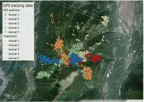
Now, you create view with a different representation of your data sets. In this case, you derive a trajectory from GPS points. You have to order locations per animal and per acquisition time; then, you can group them (animal by animal) in a trajectory (stored as a view):
CREATE VIEW analysis.view_trajectories AS SELECT
animals_id,
ST_MakeLine(geom)::geometry(LineString,4326) AS geom FROM
(SELECT animals_id, geom, acquisition_time FROM main.gps_data_animals
WHERE geom IS NOT NULL ORDER BY
animals_id, acquisition_time) AS sel_subquery GROUP BY
animals_id;
COMMENT ON VIEW analysis.view_trajectories IS 'GPS locations - Trajectories.';
In Fig.5.3, you can seeanalysis.view_trajectoriesvisualised in QGIS. Lastly, create another view to spatially summarise the GPS data set using convex hull polygons (or minimum convex polygons):
CREATE VIEW analysis.view_convex_hulls AS SELECT animals_id, (ST_ConvexHull(ST_Collect(geom)))::geometry(Polygon,4326) AS geom FROM main.gps_data_animals WHERE
geom IS NOT NULL GROUP BY
animals_id ORDER BY animals_id;
COMMENT ON VIEW analysis.view_convex_hulls IS 'GPS locations - Minimum convex polygons.';
The result is represented in Fig.5.4, where you can clearly see the effect of the outliers located far from the study area. Outliers will be filtered out inChap. 8.
This last view is correct only if the GPS positions are located in a relatively small area (e.g. less than 50 km) because the minimum convex polygon of points in geographic coordinates cannot be calculated assuming that coordinates are related to Euclidean space. At the moment, the functionST_ConvexHulldoes not support thegeographydata type, so the correct way to proceed would be to project the GPS locations in a proper reference system, calculate the minimum convex polygon and then convert the result back to geographic coordinates. In the example, the error is negligible.
Fig. 5.3 Visualisation of the view with the trajectories (zoom on the study area)
Vector Data Import and Export
There are different ways to import a shapefile. Compared to the use of tabular data, e.g. in .csv format, the procedure is even easier because users do not have to create an empty table before loading the data. The existing import tools do this job automatically (although in this way you lose control over the data type definition). In QGIS there are two plugins that support shapefile import into PostGIS. The QGIS plugin ‘PostGIS Manager’ can do the job with a drag-and-drop procedure. Together with the PostGIS installation, a useful tool is automatically created: ‘PostGIS Shapefile Import/Export Manager’ (located in the PostGIS installation folder). The same kind of tool can also be called from within pgAdmin (in the ‘plugin’ menu). The same result can be achieved usingshp2pgsql15, a command line tool. If the original file uses some specific encoding with characters not supported by standard encoding, the option ‘-W’ can be used to solve the problem. Another way to import shapefiles is with the GDAL/OGR16 library. In general, with any tool, when you load the data, you have to correctly define the reference system, the target table name and the target schema. If the original layer has errors (e.g. overlapping or open polygons, little gaps between adjacent features) it might not be correctly imported and in any case it will probably generate errors when used in PostGIS. Therefore, we strongly recommend that you control the data quality before importing layers into your database.
If you want to export your (vector) spatial layer stored in the database, the easiest way is to load the layer in a GIS environment (e.g. QGIS, ArcGIS) and then simply export to shapefile from there. The ‘PostGIS Manager’ plugin in QGIS offers advanced tools to perform this task. You can export part of a table or a processed data set using an SQL statement instead of just the name of the table. You can also use the tools mentioned above for data import (pgsql2shp, GDAL/ OGR library (ogr2ogr), PostGIS Shapefile Import/Export Manager).
Connection from Client Applications
One of the main advantages of storing and managing your data in a central database is that you can avoid exporting and importing your data back and forth between different programs, formats or files. Some client applications commonly used in connection with PostgreSQL/PostGIS have specific tools to establish the link with the database (e.g. pgAdmin, QGIS, ArcGIS 10.x). However, as you are likely using different programs to analyse your data, you need to be able to access the database from all of them. This problem can be solved using the Open DataBase Connection (OBDC) which is a protocol to connect to a database in a
15 http://www.bostongis.com/pgsql2shp_shp2pgsql_quickguide_20.bqg. 16 http://www.gdal.org/ogr2ogr.html.
standardised way independent from programming languages, database systems and operating systems. ODBC works as a kind of universal translator layer between your program and the database. Virtually any program that is able to handle data today supports ODBC in one way or another.
In Chap. 10, you will see how to use a PosgreSQL/PostGIS database in connection with R.
Special Topic:Create an ODBC driver in MS Windows
In the Windows operating system, you can easily create an ODBC connection to your PostgreSQL database. First, you have to install the PostgreSQL ODBC driver on your computer17. Then you go to ‘Control Panel—Date Sources (ODBC)’ or ‘Microsoft ODBC Administrator’ (according to Windows version), select ‘System DSN’ tag and click ‘Add’)18. Select ‘PostgreSQL Unicode’ and the appropriate version (32 or 64 bit, according to PostgreSQL and ODBC Administrator versions), and fill the form with the proper connection parameters. You can check whether it works by clicking ‘Test’, then click ‘Save’. Now you have the ODBC connection available as system DSN. ‘Data Source’ is the name that identifies the ODBC driver to your database. Once created, you can access your database by calling the ODBC driver through its name. You can test your ODBC connection by connecting the database from, e.g. MS Excel. Sometimes a spreadsheet is useful to produce simple graphics or to use functions that are specific to this kind of tool. To connect to your database data you have to create a connection to a table. Open Excel and select ‘Data—Connection’ and then ‘Add’. Click on the name of the ODBC driver that you created and select the table you want to open in MS Excel. Go to ‘Data—Existing connections’ and select the connection that you just established. You’ll be asked where to place this data. You can choose the existing worksheet or specify a new worksheet. Take your decision and press OK. Now you have your database data visualised in an Excel spreadsheet. Spatial data are visualised as binary data format, and therefore they cannot be properly ‘read’. If you want to see the coordinates of the geometry behind, you can use a PostGIS function likeST_AsTextorST_AsEWKT. Tables are linked to the database. Any change in Excel will not affect the database, but you can refresh the table in Excel by getting the latest version of the linked tables.
References
Corti P, Mather SV, Kraft TJ, Park B (2014) PostGIS Cookbook. Packt Publishing LTD., Birmingham, UK
Obe OR, Hsu LS (2011) PostGIS in action. Manning Publications Company, Greenwich
17 http://www.postgresql.org/ftp/odbc/versions/msi/.