Performance analysis and optimization of a distributed processing framework for data mining accelerated with graphics processing units

Master on Information Technologies for Business

Intelligence

Performance Analysis and Optimization

of a Distributed Processing Framework

for Data Mining Accelerated with

Graphics Processing Units

IT4BI MSc Thesis

Student:

Edgar Isaac HiroshiLeon Saiki Supervisors: Dr. Toon Calders, Nam-LucTran, Sabri _Skhiri Barcelona, September 2014

Abstract

Facultat d’Inform`atica de Barcelona

MASTER ON INFORMATION TECHNOLOGIES FOR BUSINESS INTELLIGENCE

Performance Analysis and Optimization of a Distributed Processing Framework for Data Mining Accelerated with Graphics Processing Units

by Edgar Isaac HiroshiLeon Saiki

In this age, a huge amount of data is generated every day by human interactions with services. Discovering the patterns of these data are very important to take business decisions. Due to the size of this data, it requires very high intensive computation power. Thus, many frameworks have been developed using Central Processing Units (CPU) implementations to perform this computation. For instance, a distributed and parallel programming model such as Google’s MapReduce. On the other hand, since the last half decade, researchers have started using Graphics Processing Units (GPU) performance to process these huge data. Unlike CPU, GPU can execute many tasks in parallel. To measure the performance of GPU, EURA NOVA implemented two data mining algorithms (K-Means and Naive Bayes) in the framework to enable task execution in a distributed manner by considering availability of GPU power in each node. Even though the framework was successfully implemented, when compared to another CPU parallel framework, its performance was very poor. It shows that the framework does not use the performance of GPU effectively. Moreover, it contradicts with the fact that GPU can execute many tasks in parallel and thus, faster than CPU implementation. As a result, this research topic started with the objective to answer how to improve this performance. Specifically, to improve the performance of the K-Means implementation. We also included a new data mining implementation called Expectation Maximization to the framework, taking advantage of each GPU node and the distribution nodes. Furthermore, we address some good practices when implementing data mining in GPU from a sequential design.

Working with general purpose GPU is still in development stage. A well known library is Thrust. We used it to achieve the above objectives. Finally, we evaluated our solutions by comparing with other existed CPU frameworks. The results show that we improved the K-Means performance more than 130x, and plugged the expectation maximization implementation into EURA NOVA’s framework.

I would like to express my deep gratitude to my supervisor Professor Toon Calders and EURA NOVA’s Advisors: Nam-Luc Tran and Sabri Skhiri. For their patient guidance, enthusiastic encouragement and useful critiques of this research work.

I will always be in gratitude with Consejo Nacional de Ciencia y Tecnologia (CONA-CYT), the organization which granted me and gave me the opportunity to further continue my studies. As well as EURA NOVA, a young company founded in 2008, established in Belgium, where I did my master thesis.

I would also like to thank Dr. Jorge, Arnaud, Sahilu, Olivier and Alexander, for their advice and assistance during my master thesis. My grateful thanks are also extended to my IT4BI colleagues for their help during all the semesters as well as keeping me motivated.

My deepest appreciation to my parents, for always being supporting and caring for me during my entire life. Also, for encourage me throughout all my studies. Life could not have given me better parents, love you.

I would (particularly) like to thank Mitsue, without her, this would not had been pos-sible, she is a role model to me. Also, I want to thank Sashiko and my aunt Chela for always cheering me up, love you all.

Finally, I am deeply grateful to Brenda, for all her support for so many years, as well as always being there when I needed her the most, love you.

Abstract ii

Acknowledgements iii

Contents iv

List of Figures vi

List of Tables viii

1 INTRODUCTION 1 1.1 Context . . . 1 1.2 Motivation . . . 3 1.3 Scope . . . 5 1.4 Objectives . . . 5 1.5 Initial Planning . . . 6 1.6 Thesis Structure . . . 7 2 GPU Programming 8 2.1 GPU Programming . . . 8 2.1.1 GPU . . . 8

2.1.2 GPGPU - General-Purpose computing on Graphics Processing Units 9 2.1.3 GPU Programming model . . . 9

2.1.4 Advantages and Disadvantages of programming with GPU . . . . 11

2.1.5 CUDA . . . 12 2.1.6 Thrust . . . 13 2.1.6.1 Reduce . . . 14 2.1.6.2 Sort . . . 14 2.1.6.3 Fill . . . 14 2.1.6.4 Sequence . . . 15 2.1.6.5 Transform . . . 15 2.1.6.6 Sort by key . . . 16 2.1.6.7 Reduce by key . . . 16 2.1.6.8 Count . . . 17 2.1.6.9 Repeated Range . . . 17 iv

3 MapReduce 18 3.1 MapReduce . . . 18 4 DATA MINING 21 4.1 Data Mining . . . 21 4.1.1 K-Means . . . 22 4.1.2 Expectation Maximization. . . 24

4.1.3 Data Mining Frameworks . . . 27

R . . . 27

Weka. . . 27

Mahout . . . 27

4.2 SNIFF - Parallel Implementation of K-Means using GPU . . . 28

4.3 Related Work . . . 30

4.3.1 K-Means Frameworks Implementations . . . 30

4.3.1.1 Mahout Parallel K-Means . . . 30

4.3.1.2 R K-Means . . . 34

4.3.1.3 Weka K-Means . . . 35

4.3.2 Literature survey . . . 36

5 CONTRIBUTIONS 38 5.1 Data Mining Using GPU Requirements - Review . . . 38

5.2 Data Mining Frameworks K-Means implementations analysis . . . 39

5.3 Methodology . . . 40

5.4 Further Optimizations . . . 47

5.5 Expectation Maximization Implementation in SNIFF . . . 53

6 Final Planning 55

7 CONCLUSIONS & FUTURE WORK 56

A Dataset 58

B Source Code 59

1.1 Average time spent on the computations of models. The figure on the left shows the average time spent on the computation of the model on 3 GPU nodes, on a single GPU node and on a CPU node for various sizes of the dataset for the Naive Bayes implementation. The figure on the right presents the average time spent on the computation of one K-Means iteration on a GPU node and on a CPU node for various sizes of

the dataset [1]. . . 2

1.2 Average time spent for the computation on a GPU node Titan (Nvidia Graphics card [2]) and on the Mahout for one iteration time using various sizes of the dataset. Each of the nodes in the cluster locally processes one third of the total data size. In the case of Mahout, the data will be processed depending of how the data was distributed by Hadoop [3], using default block size of 64MB. . . 3

1.3 DFG representation of a job [1].. . . 4

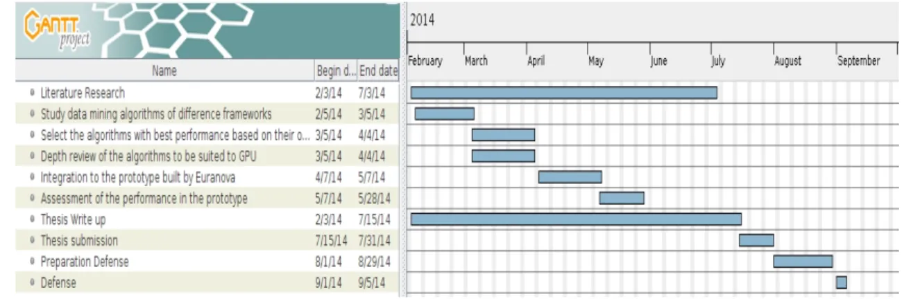
1.4 Initial Planning for the master thesis . . . 6

2.1 GPGPU Timeline adapted from [4]. . . 9

2.2 GPU kernel structure and invocation [5].. . . 10

2.3 The threads are contiguous having good performance [6]. . . 10

2.4 The threads are random having bad performance [6]. . . 11

3.1 The MapReduce framework breaks down data processing into map, shuf-fle, and reduce phases [7]. . . 19

3.2 MapReduce Word Count example flow [8]. . . 19

4.1 The Knowledge Discovery Process . . . 21

4.2 Initial centroids (Green, Blue and Red dots) and datapoints (gray dots) [9]. 22 4.3 Each datapoint is assigned to its nearest centroid [9]. . . 23

4.4 Recalculate the centroids based on the datapoints assignations [9]. . . 23

4.5 New cluster values [9]. . . 23

4.6 Observations in which the gaussian models are already known [10]. . . 24

4.7 Observations where the gaussians are not known [10]. . . 24

4.8 First iteration [10]. . . 24

4.9 Result of first iteration [10] . . . 25

4.10 Result of second iteration [10] . . . 25

4.11 Expectation step [11]. . . 26

4.12 Maximization step [11]. . . 26

4.13 Architecture of SNIFF framework. All workers are equipped with a GPU and in order to process the data, each worker needs to register to a mas-ter node, in which they receive instructions, job information and clusmas-ter

configuration. Step 3 a and b may be repeated [1]. . . 28

4.14 Distributed K-Means - Worker Routine [1]. . . 29

4.15 Distributed K-Means - Combiner Routine [1]. . . 29

4.16 Mahout K-Means Implementation [12]. . . 31

4.17 Distributed K-Means - Map Phase. . . 32

4.18 Distributed K-Means - Combiner Phase. . . 33

4.19 Distributed K-Means Mahout- Reduce Phase. . . 33

4.20 K-Means R implementation [13]. . . 35

4.21 K-Means Weka implementation.. . . 36

5.1 Flowchart with all the steps to identify potential bottlenecks . . . 40

5.2 Average time spent for one iteration when computing all the distances with the datapoints and the centroids, and assigning the datapoints to the clusters on a GPU Node (Titan) in SNIFF and in one node of Mahout CPU. . . 42

5.3 Comparison of the average time spent in one iteration on a GPU Node (Titan) and with the total time spent when computing the distances and the assignation of the datapoints to their centroids. . . 43

5.4 Comparison of the average time spent when computing distance of one centroid with one datapoint using 100, 1000, 10,000, 100,000, 1,000,000 and 10,000,000 iterations for a GPU Node (Titan) and in one CPU node when running Mahout K-Means. . . 44

5.5 Average time spent for the computation on a GPU node (Titan) and on the Mahout for one iteration time disabling and enabling compiler optimizations for SNIFF. NEWSNIFF has more than 90x speed up per-formance compared to SNIFF, and 10x compared to Mahout. . . 46

5.6 Average time spent for the computation on a GPU node (Titan) and on new SNIFF for one iteration time after using new implementation of Reduce by key. . . 52

5.7 Distributed Expectation Maximization Worker Routine. . . 53

5.8 Distributed Expectation Maximization Combiner Routine. . . 54

5.9 EM Average time for the computation on a GPU node (Titan) for one iteration . . . 54

2.1 GPU Advantages and Disadvantages . . . 11

5.1 Example of the data formats . . . 41

5.2 Example of the data . . . 47

5.3 Result of the sum of the values for each datapoint . . . 48

5.4 The input of Reduce by key are two vectors in 1 dimension: the vector keys and the vector values. . . 48

5.5 The output of Reduce by key are two vectors in 1 dimension: the keys and the values. . . 49

5.6 The vectors with all the dimension values in 1 dimension. . . 50

5.7 The vector with the keys. . . 50

5.8 The input vector with all the keys. . . 50

To my family, specially to my

brother Katzuo, miss you so

much...

INTRODUCTION

1.1

Context

Nowadays, lots of important data are generated in our daily life. These data are used by companies to take business decisions by using data mining techniques analyzing the meaning of this data [1]. As per pingdom website [14], data on the web is growing expo-nentially and there are more than two billion users generating data by interacting with services. Data mining is a field of computer science that plays a vital role in different areas of applications, like healthcare, market analysis, manufacturing, engineering, etc [15]. To enable the analysis of massive amounts of data in a reasonable time, parallel computing has been used and is getting huge attention since the past decade. Further-more, in the past years we have seen the development of general purpose computing on Graphics Processing Units (GPU) [1], since GPUs [16] can theoretically deliver more parallel computing performance than traditional CPUs [17].

In GPU programming, there are different programming models which depend on the type of GPU device. For instance, the most commonly used programming models are CUDA [18] and OPENCL [19]. CUDA can only be used by Nvidia [18] GPU devices, whereas OPENCL can be used in any type of GPU Devices. On the other hand, it is also necessary to deal with memory allocation and memory access patterns [1]. There are some libraries that can deal with such low-level hardware considerations. For example, Thrust [20] is a library that contains parallel algorithms [21]. Thrust also presents good practices for using the GPU in general purpose computing [1].

There are two types of parallelism presented in EURA NOVA’s implementation:

• Per node GPU, allowing further parallelism within each of the nodes.

• Multiple nodes, each equipped with its own CPU and Memory and connected with a network.

Per node GPU, where each node equipped with a GPU can execute its routine in paral-lel. Multiple nodes, where the program can be executed in the cluster to run in paralparal-lel. These two together add a second level of parallelization, making the performance of the computation faster [1]. SNIFF [1] is an appropriate framework for data mining that ex-ploits both types of parallelism simultaneously. SNIFF was developed by EURA NOVA in order to prove that these two types of parallelism can achieve better computation for the GPU than its counterpart CPU.

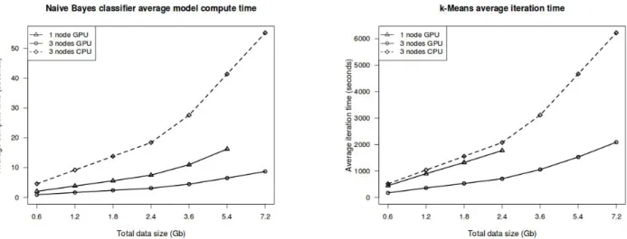
In order to validate the framework and the execution model, Tran et al. [1] developed parallel GPU and CPU versions of two data mining algorithms in SNIFF: the Naive Bayes classifier [22] and the K-Means clustering algorithm [23]. These two algorithms were implemented in a distributed cluster system exploiting the massive parallel com-putation provided by the GPU in each node. The SNIFF framework resulted in a performance gain for the two aforementioned data mining problems for the GPU im-plementation outperforming the CPU imim-plementation. The results are presented in the following graph [1]:

Figure 1.1: Average time spent on the computations of models. The figure on the left shows the average time spent on the computation of the model on 3 GPU nodes, on a single GPU node and on a CPU node for various sizes of the dataset for the Naive Bayes implementation. The figure on the right presents the average time spent on the computation of one K-Means iteration on a GPU node and on a CPU node for various

Therefore, one can add more value and form a proper platform for distributed hetero-geneous processing in the future by combining the best of the distributed processing models and the parallel processing capabilities of the GPUs [1].

The performance of K-Means GPU implementation in the SNIFF framework was tested with a Dataset of KDD Cup 1999 (Appendix A) with different sizes from 0.6 Gb to 7.2 Gb. The same dataset was applied to the CPU K-Means implementation of Mahout [24], which is another data mining framework exploiting parallel computation on a cluster.The starting point of this thesis was the observation that the results of SNIFF GPU K-means implementation were considerably slower than that of the Mahout CPU K-means, as can be seen in the following graph:

Figure 1.2: Average time spent for the computation on a GPU node Titan (Nvidia Graphics card [2]) and on the Mahout for one iteration time using various sizes of the dataset. Each of the nodes in the cluster locally processes one third of the total data size. In the case of Mahout, the data will be processed depending of how the data was

distributed by Hadoop [3], using default block size of 64MB.

Theoretically, the GPU version has to be faster than the CPU version for computing tasks that require intensive computation. Therefore, the main goal of this project was to make the GPU implementation faster and find good practices to optimize the data mining implementations using GPU.

1.2

Motivation

Apart from the CPU, there are other different architectures that can be used to process the data, such as GPU [25]. GPU took their first steps as graphics accelerators, but nowadays, they are becoming more programmable and researchers started to use GPUs

for non-graphics applications too [25]. Typically, graphics hardware contains a large number of programmable processors which are optimized to work efficiently, providing extremely high parallelism.

Nowadays, clusters with GPUs are being used throughout the world. Three of the five largest supercomputers in the world employ GPUs [25].

Researchers in data mining have demonstrated the superiority of the computational power of parallel processing in GPUs over that of CPU. For instance, in [26], the authors selected two clustering algorithms, the density-based algorithm DBSCAN [27] and the iterative algorithm K-Means. Both implementations using GPU outperformed their CPU counterparts. Other related works regarding K-Means implementations have shown significant speed ups as compared to their CPU counterparts [28–31]. Similar results were also obtained for K Nearest Neighbors implementation [32].

For EURA NOVA, the outcome of this thesis is not only important for optimizing the K-Means implementation for SNIFF and reviewing best practices in Data Mining using GPU. But also the insights in parallel programming obtained in the project could be used and add value in other projects of EURA NOVA, such as Arom [33]. The Arom project, which is based on a DataFlow Graph (DFG), can run distributed parallel data processing jobs on high volumes of data. The DFG model [1] is a graph where the operations are represented by nodes and data dependencies between operations are on the edges. Tran et al. [1] believe that an extension to the DFG model, e.g. Arom or Dryad [34], can be made using GPU, forming a suitable platform for distributed heterogeneous processing. As shown in the following figure [1]:

Figure 1.3: DFG representation of a job [1].

This DFG job contains two data sources, preprocessing stages and a join operation. Their results are the input to a GPU-enabled operation stage, represented as the squared nodes in the figure 1.3 [1].

1.3

Scope

The initial step of this research was to study the existing implementations of data mining algorithms from differents frameworks, such as Mahout [24], R [35] and Weka [36]. We mainly focused on the Mahout’s K-Means implementation, since this implementation outperformed EURA NOVA’s K-Means GPU implementation in an earlier study done by EURA NOVA. In the case of R and Weka, we focused in the sequential implementations to get some insights that may help to optimize the GPU K-Means implementation in SNIFF.

In addition, it was required to do a review of the conditions to efficiently execute data mining algorithms using GPUs. It was necessary to take into account some consider-ations when working with GPU, because a bad parallel implementation can lead to a terrible performance [1]. In this respect, Cristian Bohm et al. [26] proposed some data mining algorithms using GPUs. This review could help future works using data mining with GPU.

This study focused on optimizing a K-Means implementation in EURA NOVA’s work called SNIFF, as well as taking into account the differences of the optimized frame-works’ implementations to integrate them in SNIFF. The study also included relevant information about best practices of Data Mining using GPU. As a result, the distributed processing framework for data mining with GPU built by EURA NOVA should have bet-ter time performance execution afbet-ter optimizing the implementation.

1.4

Objectives

The first three goals of this master thesis according to [37] were:

1. To provide an analysis of the existing data mining algorithms and optimization of reference data mining frameworks such as Mahout, R and Weka.

2. To provide an in-depth review of the requirements for data mining algorithm to be optimally suited for GPUs.

3. To integrate the optimized algorithms into the prototype built by EURA NOVA.

4. As well as providing an implementation in the SNIFF framework of Expectation Maximization (EM) [38].

Regarding the implementation of the EM, we took it into consideration since EM is another algorithm that can be distributed and requires intensive computation. We

will also give an insight of how this algorithm can fit the SNIFF framework using the capabilities for each node of GPU.

1.5

Initial Planning

The first step was to start by doing a “literature research” to study some of the algo-rithms of the frameworks previously mentioned. After doing this study, the following step was to start with an in-depth review of the requirements for the data mining al-gorithms to be suited for using a GPU. Consequently, all the optimizations will be implemented in the prototype already built by EURA NOVA [1]. After some tests, the execution time performance of the framework should be better, based on the op-timizations of these implementations of the algorithms. If problems arise, then it may be necessary to review the implementations again. All the observations of the thesis should be written, making sure to understand the implementations of the algorithms of the open source frameworks and how these were optimized along with the requirements in order to use the best practices, so the GPU can work as efficient as possible.

Timeframe estimation for the Initial Planning:

1.6

Thesis Structure

In the following chapters, relevant background information will be provided. Chapter 2 provides scientific background for GPU programming as well as some good practices using Thrust library. In chapter 3, a brief introduction of Map Reduce is presented since it was the parallel technique used in the K-Means CPU implementation of Mahout. In chapter 4, information regarding Data Mining is presented, containing K-Means and Expectation Maximization, as well as the parallel implementation of K-Means using the SNIFF model. Related Work is also presented in this chapter, which includes an anal-ysis of different frameworks making K-Means available and Literature survey. Chapter 5 contains the contributions of the thesis. This chapter includes a review of the re-quirements for the best practices using GPU and Data Mining, an analysis for the data mining frameworks regarding K-Means, as well as the methodology that was followed for optimizing SNIFF K-Means, further optimizations and the Expectation Maximization in the SNIFF model. In chapter 6, Final planning will mention some minor changes of the initial planning. Finally, chapter 7 includes Conclusions & Future Work.

GPU Programming

In this chapter, we will explain basic concepts of GPU Programming. We will high-light some important structures illustrated with examples, which are very common at programming with GPU using Thrust Library.

2.1

GPU Programming

At first, GPUs were only used as 3D accelerators; nowadays, GPUs are also being used to speed up general-purpose computations. Due to their massive parallelism, they are well-suited for executing many similar tasks in parallel [1]. In this section, characteristics of the GPU are presented as well as the GPU programming model. We will mention some of the main advantages and disadvantages of programming with GPU. An extension of C programming language called CUDA will be presented since it was the one used during the experiments of SNIFF due to its simplicity and performance compared to other languages using GPU [39] such as OpenCL. Finally, Thrust Library, which simplifies CUDA programming, will be presented.

2.1.1 GPU

GPU [16] is a processor which is in charge of handling graphical tasks. A GPU is similar to a CPU. Nevertheless, a GPU is specifically designed to perform complex mathematical and geometric calculations that are required for graphics rendering, since it can draw multiple pixels in parallel. CPU and GPU process their tasks differently. A CPU contains few cores optimized for sequential serial processing while a GPU consists of thousands of smaller cores designed for handling multiple tasks simultaneously [40]. At the beginning, GPUs were made specially for graphics accelerators; nevertheless, their

power can also be used for non-graphics applications, called General-Purpose Computing on Graphics Processing Units [1].

2.1.2 GPGPU - General-Purpose computing on Graphics Processing Units

Figure 2.1: GPGPU Timeline adapted from [4].

At first, GPUs were used as graphics accelerators; however, in 2000, researchers started to use these graphics adapters for non-graphics applications [25]. Programming for the GPU [25] was very challenging because deep knowledge of the GPU architecture was required and it was available only for people who were familiar with graphics processing language, e.g. OpenGL or Direct3D. However, Ian Buck et al. [41] developed a system for General Purpose Computation on GPU called Brook. Brook was a C extension that made easier for a wider audience to use GPU Processing. Ian Buck and other developers released CUDA in 2006. CUDA is a parallel computing platform and programming model for general-purpose computation. In 2008, the Khronos Group released a cross-platform parallel programming model OpenCL 1.0 a competitor of CUDA.

2.1.3 GPU Programming model

A program for GPU is separated into two parts [25]: The host code and the kernels. The host code is executed on the CPU and the kernels on the GPU. The host code in the CPU will be in charge of running the main program and sending directions to the GPU, launching the kernels. A kernel is a program that is executed on the GPU; all threads in a kernel perform the same tasks, the difference is the data that is processed. A kernel is a grid of blocks, where each block is assigned to a streaming multiprocessor (SM) and can contain 1024 threads as maximum. The execution is divided into groups of 32 threads, called warps, that run at the same time, instead of executing the 1024

threads that are on a block [25]. The number of warps composed of 32 threads can be many in the GPU depending on the number of cores of the GPU. These will be executed in parallel and the remaining threads will be waiting till the others warps finish in order to be executed. The following figure represents a kernel launch that will store a block of threads in a grid and in each block containing these threads [5]:

Figure 2.2: GPU kernel structure and invocation [5].

In order to have a great performance when running the kernel, these are some of the challenges proposed by [25]:

1. Graphics devices only offer limited synchronization possibilities.

2. Memory access should be coalesced to fully utilize the high bandwidth of device memory. Coalesced is an access pattern where each thread access a consecutive block of memory without any gaps. This results in a great performance since whenever each thread wants to read or write to the global memory, it always access a large chunk of memory; the GPU can reuse this large chunk of memory for all the threads that are contiguous, giving better performance than if the access was randomly done [6]. As can be seen in the following pictures:

Figure 2.4: The threads are random having bad performance [6].

3. Divergence at warp level should be avoided.

Divergence [25] in the GPU is present when some threads take a different execution path when evaluating a condition. When threads take different code paths, since there is a single program counter per SM, the execution is serialized and part of the processor idle. The best way to have a good performance is that all threads that are assigned to a SM execute the same instruction per cycle. In the case of inter-warp, since they are in different warps, divergence is not an issue. This execution in GPU is called SIMT (Single Instruction, Multiple Threads). The CPU programming model [25] follows the execution of SIMD (Single Instruction, Multiple Data), in which it allows each thread to branch.

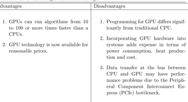
2.1.4 Advantages and Disadvantages of programming with GPU

Some advantages and disadvantages of programming with GPU are presented in the following table [25,42]:

Table 2.1 GPU Advantages and Disadvantages

Advantages Disadvantages

1. GPUs can run algorithms from 10 to 100 or more times faster than a CPUs.

2. GPU technology is now available for reasonable prices.

1. Programming for GPU differs signif-icantly from traditional CPU.

2. Incorporating GPU hardware into systems adds expense in terms of power consumption, heat produc-tion and cost.

3. Data transfer at the bus between CPU and GPU may have perfor-mance problems due to the Periph-eral Component Interconnect Ex-press (PCIe) bottleneck.

2.1.5 CUDA

CUDA [18] is a parallel computing [43] platform and programming model created by Nvidia; it improves the computing performance by harnessing the power of the GPU. CUDA takes advantage of heterogeneous systems that have both CPUs and GPUs [44]. A CUDA program is split into two parts: The host code, which is the code executed in the traditional CPU, and The device code, which runs on the GPU [44].

We illustrate the advantage of using GPU vs CPU with an example from [45]. In this example, 100 numbers need to be squared. The following fragment shows how to code this task for CPU:

for(i=0; i<100; i++) {

output[i] = input[i] * input[i]; }

This previous code is only launching one thread at a time in which is putting the result of the multiplication done by the input array in the output array, and it loops 100x times, one thread after another. In the case of the GPU, it is possible to just run a program called kernel in which it will launch for this example 100 threads at the same time in a block, as oppose to the previous CPU example, making the square of each number of the array, as shown with the following code:

square<<<1, 100>>>(d_out, d_in); //Kernel, launching 100 threads in 1 block square(output, input){

idx = threadIdx.x; //Each thread contains an id.

f = input[idx]; //Based on this id, the value is stored in f output[idx] = f * f; //The square of the numbers in

//f is stored in output array }

Appendix B contains the full implementation of the CUDA code retrieved from [45]. It describes all the previous procedures for launching the kernel, such as memory allocation from the CPU to the GPU. Note that to launch a Kernel you have to allocate memory from CPU to the GPU and then process the data in the GPU. Finally, the result must be copied back from the GPU to the CPU. In CUDA, there is a library called Thrust [46], which allows the users to implement parallel applications, making it easier to be implemented since it reduces many complexities that will be explained in the following section.

2.1.6 Thrust

Thrust is a library based on the C++ standard template library and it is fully inter-operable with CUDA [46]. Thrust helps the programmers to write GPU applications efficiently and with minimum effort, since it contains very efficient implementations of algorithms such as sort, transform, reduce, etc.

Using Thrust, the developers describe their computation using the algorithms that are provided by the library and completely delegate how to implement the computation to Thrust. This allows the programmers to describe only what to compute without additional restrictions on how to carry out the computation [20]. For example by not having to deal with all the detailed complexity of memory allocation such as in pure CUDA code.

Features of Thrust can be presented in the following examples that were retrieved from [20]. A Thrust program which sort data on the GPU [20]:

int main (void) {

//generate 16M random numbers on the host thrust::host_vector <int> h_vec (1 << 24); // transfer data to the device

thrust::device_vector <int> d_vec = h_vec; // sort data on the device

thrust::sort(d_vec.begin(), d_vec.end()); //transfer data back to host

trust::copy(d_vec.begin(), d_vec.end(), h_vec.begin()) }

Thrust provides two vector containers: host vector and device vector. The host vector is stored in the RAM memory and the device vector in the memory of the GPU. As shown in the previous example, after generating random numbers in the host vector it will allocate and transfer the data into the device memory, then the sorting function will be executed in the GPU for all the values contained in the device vector. Finally, the result is transferred to the host vector using the copy instruction from Thrust. Note that running the sort function may imply launching one or more CUDA Kernels but all these are abstracted, so the programmer does not have to deal with the launch configuration of the kernels, Thrust library does it for you [20].

Some of the common implementations and examples of Thrust parallel algorithms exe-cuted in the GPU along with their descriptions are presented next [46]:

2.1.6.1 Reduce

A reduction algorithm uses a binary operation to reduce an input sequence to a single value, e.g. the sum of an array of numbers is obtained by reducing the array. If no binary operation is specified, the elements will be summed by default (+ operation). As an example, suppose we have one input vector with these values:

Vector 10 20 50 20

The output of the following function:

int Sum = thrust::reduce(Vector.begin(), Vector.end());

will have a value with the sum of all the elements: Sum 100

2.1.6.2 Sort

Thrust offers several functions to sort data or rearrange data according to a given crite-rion. By way of illustration, we have this input vector:

Vector 3 2 1 5 4

The output of the following function:

thrust::sort(Vector.begin(), Vector.end());

will be a sort the vector in ascending order:

Vector 1 2 3 4 5

2.1.6.3 Fill

Simply sets a range of elements to a specific value. For example, this input vector with 0 values:

Vector 0 0 0 0 0 0 0

After the following function:

thrust::fill(Vector.begin(), Vector.end(), 7);

The vector will contain the value 7 in all its elements:

2.1.6.4 Sequence

A function can be used to create a sequence of equally spaced values. As a case in point, this input vector with 0 values:

Vector 0 0 0 0 0 0 0

The following function:

thrust::sequence(Vector.begin(), Vector.end());

will fill the vector with the following sequence:

Vector 0 1 2 3 4 5 6

2.1.6.5 Transform

Transform applies a unary function to each element of an input sequence and stores the result in the corresponding position in an output sequence. Specifically, an operation is performed for each element i in the range and the result is assigned to the output iterator. The input and output sequences may coincide, resulting in an in-place transformation [47]. For instance, we have two vectors as input and one as output:

Vector 5 6 9 10 20 30

Vector2 2 3 5 5 10 20

Vector3 0 0 0 0 0 0

thrust::transform( Vector.begin(), Vector.end(), Vector2.begin(), Vector3.begin(), thrust::minus<float>() );

This function will compare each element in the Vector and Vector2, and compute the difference and storing the result in Vector3. Having the following output for Vector3:

Vector3 3 3 4 5 10 10

Thrust covers most of the arithmetic operations (+, - , /, *, mod). However, often we want to do something different. For instance, there is a very well known vector operation called SAXPY operation: y<- a * x + y, where x and y are vectors and a is a constant. In this case we can implement our own function SAXPY to do this operations in a single transformation.

Vector X 2 4 6 8 10

Vector Y 5 10 15 20 25

a 10

Where saxpy is the function that will perform for a multiplication with a constant ”a” with x and a sum with Y. It is possible to compute more operations with each value in a vector just by following this saxpy example in thrust.

This function will perform the SAXPY operation y<- a * x + y :

thrust::transform(X.begin(), X.end(), Y.begin(), Y.begin(), saxpy(a));

It will output the following vector storing the results in the four parameter (Y.begin()) of the transform operation:

Vector Y 25 50 75 100 125

All the values computed by the operation are stored in Y vector by overwriting the previous values in Y; preventing to allocate memory in another vector.

2.1.6.6 Sort by key

Sort by key performs a key-value sort. By way of illustration, these two input vectors:

Keys 1 3 2 6 4 5

Values 10 20 30 50 15 25

With the next function:

thrust::sort by key(Keys.begin(), Keys.end(), Values.begin());

The output of the keys and values is:

Keys 1 2 3 4 5 6

Values 10 30 20 15 25 50

2.1.6.7 Reduce by key

Reduce by key is a generalization of reduce to key-value pairs. For each group of con-secutive keys in the range keys first, keys last that are equal, reduce by key copies the first element of the group to the keys output. The corresponding values in the range are

reduced using the plus operation and the result copied to values output. For instance, these two input vector:

KeysInput 1 3 3 3 2 2 1

ValuesInput 9 8 7 6 5 4 3

With the following function:

thrust::reduce by key(KeysInput.begin(), KeysInput.end(), ValuesInput.begin(), KeysOutput.begin(), ValuesOutput.begin());

will put the result by grouping by same keys in the two output vectors: KeysOutput and ValuesOutput:

KeysOutput 1 3 2 1

ValuesOutput 9 21 9 3

2.1.6.8 Count

Count returns the number of instances of a specific value in a given sequence. For example, this input vector: _Vector 1 3 5 2 5 7 5

This function:

int Result = thrust::count(Vector.begin(), Vector.end(), 5);

will assign to the result variable, the total number of elements with value 5: Result 3

2.1.6.9 Repeated Range

Repeated Range will create a vector with the number of repeated values according to a parameter as output. For example, the next input vector:

Vector 1 2 3 4

By assigning the value three for repetition with the following function:

repeated range <Iterator>Vector2(Vector.begin(), Vector.end(), 3);

The output will be a vector with repeated range of three for each element.

MapReduce

In this chapter, a brief introduction of Map Reduce is presented. It is the framework used by Mahout to process the data, in which the Mahout CPU implementation of K-Means was compared to the SNIFF GPU K-Means implementation.

3.1

MapReduce

Distributed systems can present many complexities [48], such as computation paral-lelization, work distribution, and dealing with unreliable hardware and software. Nev-ertheless, the MapReduce model makes parallel processing simpler by abstracting away from these complexities. MapReduce uses key/value pairs: The keys are used to identify the information and the values are the data associated with the key.

MapReduce [49] is a programming model for processing large datasets. MapReduce allows to write data-parallel programs and execute them in a distributed system.

In MapReduce a user implements two main phases [7,50]:

1. Map Phase. - The node takes the input in a set of key/value pairs, the map will produce zero or more key/value pairs as output to the Reduce Phase.

2. Reduce Phase. - The node with the reduce phase will gather all the output passed through the map phase and combine them in order to form the global output.

Between the Map Phase and the Reduce phase, there is a shuffle phase taking place. This sorts the resulting key/value pairs from the map phase by their keys; then, these pairs will be assigned to the reducer according to their keys [7].

A MapReduce program breaks down the work submitted by a client into a small paral-lelized map and reduces tasks, also called mappers and reducers. Each map task deal with a relatively small amount of data and work in parallel. The output of the map tasks are the intermediate key/value pairs that can be group by same keys before being sent to the reduce phase [7]. This grouping is also called combiner, which is an optimization by reducing the transfer time in the shuffle phase to the reduce tasks, which represent synchronization of the map tasks [7]. The following figure from [7] shows an iteration of the three phases previously explained:

Figure 3.1: The MapReduce framework breaks down data processing into map, shuf-fle, and reduce phases [7].

Word count is a typical example used for understanding MapReduce. The following figure from [8] explains the flow of using MapReduce in word count when having as input a file with 4 lines of text with a set of 3 words each:

The steps of the figure from [8] are the following:

1. Input: A file with 4 lines of text is used as input to MapReduce.

2. Split: For this example, the file is split into four sets, each set is one line from the input file.

3. Map: Each split is fed to a map() function implemented by the user, specifying the logic of how this input data will be processed. For this example, the map() function will count the occurrence of each word and adapt it to a (key, value) pair.

4. Combine: Optional step and is often used as an optimization to reduce the data transferred across the network. It is accumulating the values per mapper instead of sending each result of the map to the shuffle, thus reducing the transfer time.

5. Shuffle & Sort: Output of all the map() function is collected, shuffled, and sorted and ready to be sent to the reducer phase.

6. Reduce: The data from many map() function is aggregated and the word counts are built as (key, value) pairs.

7. Output: The output of the reduce phase is written to a file.

The main contributions of the MapReduce programming models are the scalability and fault-tolerance achieved for a variety of applications that fit this model [49].

DATA MINING

In this chapter, background for the data mining, K-Means and Expectation Maximiza-tion algorithms will be further explained, as well as informaMaximiza-tion regarding the data mining frameworks such as Mahout, R and Weka. We will also present how the imple-mentation of K-Means using GPU in SNIFF proposed by Tran et al [1], related work and literature survey.

4.1

Data Mining

Data mining is the process that can be used to discover useful and interesting pat-terns and relationships in huge quantities of data to generate rich knowledge and help organisations, government and individuals [51].

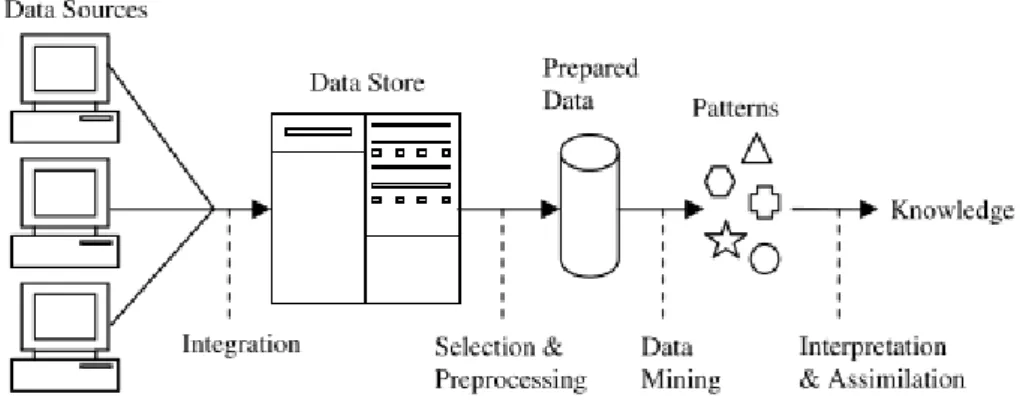
The Knowledge Discovery Process [52] is a broad process for finding knowledge in data, as illustrated in the following figure [51]:

Figure 4.1: The Knowledge Discovery Process

The Knowledge Discovery Process starts with the integration of the data, which can come from many sources. This integration places the data into a data store such as

databases or in flat files. Next, some part of the data will be selected and pre-processed into a standard format. The data mining algorithms will discover some patterns and produce an output, which will be interpreted in order to generate relevant knowledge [51]. Data Mining is just one part of the knowledge Discovery process.

Data Mining methods may be classified as either supervised or unsupervised [53]. In supervised methods, there is a particular target variable and the algorithm will have many examples where the value of the target variable is contained, meaning that the algorithm can learn from previous data. In the case of the unsupervised methods there is no target variable. Rather, the data mining algorithm searches for patterns in all the variables. The most common unsupervised data mining algorithm is clustering [53]. Clustering is the task of grouping objects which are similar to each other [51].

In the following section, two unsupervised learning algorithms will be explained: the K-Means algorithm [23] and Expectation Maximization [38].

4.1.1 K-Means

K-means clustering is an unsupervised learning algorithm [51]. The objects have to be assigned to just one of a set of clusters (group of objects). For this clustering algorithm [51], first, it is necessary to indicate the number of clusters that we want to create from the data. This number of clusters is called K. Most of the time, the value of K has a small integer value, e.g. 2,3,4, but it can be larger. It is possible to measure the quality of the clusters formed by taking the sum of the squares of the distances of each point from the centroid of the cluster to which is assigned and computing the average. We can randomly select K-clusters, but the method may work better if we pick K initial points that are fairly far apart. After selecting K initial points as shown in the following figure:

Figure 4.2: Initial centroids (Green, Blue and Red dots) and datapoints (gray dots) [9].

We assign each of the points to the cluster which has the nearest centroid. All the objects have to be assigned to just one cluster:

Figure 4.3: Each datapoint is assigned to its nearest centroid [9].

Then, based on the assignation of the points to the clusters, we recalculate the centroids of the clusters:

Figure 4.4: Recalculate the centroids based on the datapoints assignations [9].

Subsequently, we get the new cluster values:

Figure 4.5: New cluster values [9].

We keep repeating these steps until it reaches a max-limit iteration criterion or when the algorithm converges. The K-Means algorithm can do multiple rounds of processing and produces new centroids locations after each iteration [9].

In the K-Means algorithm, it is not possible to determine which number of K will produce the best set of clusters [51]. The initial selection of centroids can affect the result. This is the reason why we should run several times the algorithm for a given value of K, each time with a different choice of the initial K centroids [51].

4.1.2 Expectation Maximization

The Expectation Maximization (EM) [54] is an unsupervised clustering method which follows an iterative approach, which attempts to find the parameters of the probability distribution that has the maximum likelihood of its attributes.

Maximum-likelihood [54] can provide an estimation for the model’s parameters, such as the mean and variance, by applying this method in an observed data set and a statistical model; e.g. the Mixture model. Mixture models [10] are basically a probabilistically way of doing soft clustering, in which the datapoints can belong to any of the clusters. For each cluster, it corresponds a probability distribution, and with the EM algorithm you can discover all the parameters of the distribution for each cluster.

The following figures from [10] explain the basic concepts of Expectation Maximization. For example, there are some datapoints in which is already known that come from two gaussian models and also from which model they belong to. Thus, estimating the mean and the standard deviation for each Gaussian is trivial.

Figure 4.6: Observations in which the gaussian models are already known [10].

In the following example, it is not known the gaussian where each datapoint belongs to. Then, EM can be used to infere from which gaussian each datapoint more likely belongs to, and compute the mean and the standard deviation.

Figure 4.7: Observations where the gaussians are not known [10].

In this example, suppose we have some datapoints and two gaussian models that were put randomly in space; much like the K-Means algorithm with the K clusters.

Figure 4.8: First iteration [10].

In the EM applying soft clustering, we estimate the probability from where each dat-apoint more likely belongs to a certain distribution. In this case, the first datdat-apoint is represented in full yellow color, since it is more likely that it belongs to the yellow

gaussian for being closer to its mean. The next four datapoints have a certain proba-bility that belong to either yellow or blue gaussian according to their mean. Lastly, the following five datapoints are in full blue color since they are more likely to belong to the blue gaussian. Note: The points cannot have a 100% probability of belonging to one distribution, but in the example from [10] is shown that the closer one datapoint is to the mean of some gaussian, the more likely this datapoint belongs to that gaussian.

Figure 4.9: Result of first iteration [10]

This figure shows the result of the new gaussian or means of the second iteration, esti-mating again the probabilities using EM.

Figure 4.10: Result of second iteration [10]

EM is an extension from the basic approach of clustering [11] because, rather than assigning observations to clusters to maximize the differences in means, EM algorithm computes probabilities for each cluster based on one or more probability distributions. The objective of the EM clustering algorithm is to maximize the likelihood of the data, given the clusters [11]. In summary, EM [11] begins with an initial estimate for the missing variables and keeps iterating. In the expectation step, it finds the maximum likelihood for these variables and in the maximization step, it computes the means or the new clusters.

Expectation maximization for soft-clustering can be implemented containing four major steps [11]. To initialize, we guess the means and standard deviations; the means represent the clusters. We start with a ML hypothesis through an iterative scheme to find the final clusters k.

1. Initialization step: Initialize the hypothesis isθ0 = ( µ0₁,µ0₂, ... , µ0_k ) →Θ0_k =µ0_k

where: K is the number of Gaussians. σ is the standard deviation, θ0 is the estimate at 0th iteration,µis the mean.

2. Expectation step: Estimate the probabilities Zik of the hidden variables with

Zik will contain the probabilities of an unobserved variable i, which belongs to

cluster k.

Figure 4.11: Expectation step [11].

where: t represents the number of iteration, the values ofE(Zik) are the

probabil-ities for the hidden variables (mean and standard deviation), k is the number of the cluster,σ is the standard deviation.

3. Maximization step: Compute the new estimate of the parameters which will give the new clusters.

Figure 4.12: Maximization step [11].

4. Convergence step: if ||θt+1 _−θt_{|| < e. check whether it converged based on a}

minimum threshold or if it reached a maximum number of iterations; otherwise, keep repeating the expectation and maximization step.

4.1.3 Data Mining Frameworks

R [35] is a free programming language and software environment for statistical com-puting and graphics. Statisticians and data miners are widely using this language for data analysis. R contains numerous statistical techniques, e.g. linear and nonlinear mod-eling, classical statistical tests, classification, clustering, etc. One of the main strengths of R is the facility for producing high quality plots. R is easily extensible through func-tions and extensions. For example, advanced users can write C, C++, Java, or Python code to manipulate R objects directly [35].

Through the uses of packages, R supports a lot of data mining techniques [55], which includes: Classification and prediction, regression, clustering, text mining, Time Series Analysis, etc. Yanchang Zhao [56] presents a guide to R for data mining in a Refer-ence Sheet, which provides a comprehensive index of R packages and functions for data mining, categorized by their functionality.

Weka [36] is a collection of machine learning algorithms for data mining tasks. The algorithms can either be applied directly to a dataset or called from your own Java code. Weka contains machine learning algorithms such as classification, regression, clustering, association rules, etc [36]. These algorithms can be applied through Java code or, by the use of a graphic user interface, can be applied directly to the datasets.

Mahout [57] is a scalable machine learning library which is widely used to process large data sets. Mahout contains algorithms such as clustering, classification and collab-orative filtering which can be executed in distributed systems. They also have a version of these algorithms that can run on a single machine as well.

At the moment, Mahout supports mainly three use cases [57]:

1. Recommendation mining. - It suggests items to the users that they may like, based on understanding the user’s behaviour.

2. Clustering. - Takes, for example, text documents and groups them based on their topic.

3. Classification. - It learns from previously categorized documents which documents, of a specific category, look alike and for those documents that are unlabelled, it tries to assign them a label.

4.2

SNIFF - Parallel Implementation of K-Means using

GPU

In the following section, the parallel implementation of K-Means using GPU by SNIFF will be explained. First, SNIFF architecture will be presented in order to understand how the K-Means algorithm was implemented based on the framework.

SNIFF framework can run data processing algorithms formed by the following phases [1]:

1. Independent computation of a partial model in separate data chunks.

2. Combination of the partial models in order to compose the global model.

3. Iterate again if needed, e.g. K-Means, until a convergence criteria is met.

The following figure shows SNIFF architecture [1]:

Figure 4.13: Architecture of SNIFF framework. All workers are equipped with a GPU and in order to process the data, each worker needs to register to a master node, in which they receive instructions, job information and cluster configuration. Step 3 a

and b may be repeated [1].

Tran et al. [1] implemented a parallel K-Means algorithm based on the distributed version by [58] in the SNIFF architecture. In the SNIFF implementation, the whole dataset is partitioned equally among all the workers. Then, each node receives the same initial centroids and performs the k-means iterations on the partial data. When the iteration ends, the updated centroids position and a counter containing the data points belonging to each cluster are collected by the combiner; finally, the combiner will globally compute the centroids positions.

All the operations in K-Means algorithm are data-intensive [59] operations which can be parallelized on the GPU device. Each iteration performs the following steps in the worker node [1]:

1. Compute the distance of each data point to each of the K centroids.

2. Find the closest centroid for each data point, and use counters containing the number of data points belonging to each cluster.

3. Update each centroid according to the data points coordinates belonging to each cluster.

All the previous steps were designed in the SNIFF K-Means implementation to run on the GPU. The following figures represent the routines for the SNIFF distributed K-Means in the Worker and in the Combiner [1]. For the worker routine, we used the variables xi to represent the datapoint andmj for the clusters.

Figure 4.14: Distributed K-Means - Worker Routine [1].

4.3

Related Work

Lots of works have been going on under K-Means in different frameworks. We will also present a literature survey of K-Means GPU implementations.

4.3.1 K-Means Frameworks Implementations

In this section, we will highlight Mahout parallel K-Means implementation. Sequential K-Means implementations of R and Weka will also be discussed.

4.3.1.1 Mahout Parallel K-Means

Today, there is a need to cluster large datasets that cannot fit into memory. Mahout’s K-Means implementation can be used for large datasets using the Hadoop framework [12].

In order for Mahout to process the data, it is necessary to have it in numerical repre-sentation, if the data is not numerical, it will need to be preprocessed. Afterwards, this data should be converted into vectors and finally into a sequenceFile which is a specific Hadoop file format [12].

The K-means implementation in Mahout receives the following input parameters [9]: • A SequenceFile containing the input vectors.

• A SequenceFile with the initial cluster centers, which can be random.

• A similarity measure, e.g. Euclidean distance, Cosine distance, Manhattan dis-tance, etc.

• A convergence threshold.

• A maximum number of iterations in case there is no convergence first.

• The vector implementation used for the input files.

As an output, you get the final centroids coordinates and the samples attributed to each cluster. The output files are in SequenceFile format. Mahout provides some libraries in order to convert txt files and create the vectors that will be the input for the K-Means implementation [12].

According to [12], Mahout K-means contains three stages: 1. Initial stage: the dataset will be split into many blocks.

2. Map stage: In each map function, it reads the centroids in memory first, and then it will calculate the distances between the objects and the cluster centroids; the objects will be assigned to the nearest cluster centroid. Each map task is processed within a data block. Each key represents a datapoint where it will store the index to which cluster it belongs to, and the value contains the dimensions values of the datapoint.

3. Reduce stage: In the reduce function, the cluster’s centroid will be recalculated in that cluster. Also for each of the clusters in the reduce phase it will calculate whether the cluster converged or not. If the algorithm converged, then the itera-tions loop finish, otherwise it will continue until it reaches the maximum number of iterations.

The three stages of Mahout K-means are represented in the following figure from [12] :

Figure 4.16: Mahout K-Means Implementation [12].

In Mahout there are two types of implementation of K-means: Sequential and using MapReduce. The focus will be in the Map-Reduce implementation, since it is distributed in different nodes, like the SNIFF K-Means.

The main steps of the pseudo code were taken from [60] and from the implementation in version 9 of Mahout K-Means [24] which are located in lines [4,7-8,11-18]. Each instance represents a record in the dataset. The following steps describe the Mahout K-Means implementation at a higher level, whereas an instance represents just one datapoint:

Figure 4.17: Distributed K-Means - Map Phase.

Note that in line 7, an square root is applied after the distance computation of the datapoint with the centers. Also, instead of using the minimum distance to compute the new centroid, lines [8-9, 11-13] are transforming the distance into a probability, where the centroid closest to the instance will contain higher probability. On the contrary, the instance that are further from the centroids will have less probability. Lines [14-16] will assign to the index variable the position of the cluster for the instance which contains the highest probability.

Mahout’s K-Means implementation also contains a combiner which is an optimization that will partially sum the instances assigned to the same cluster; thus, decreasing the number of intermediate keys that are being passed to the reducer. To compute the global mean, it is necessary to record the number of samples in the same cluster of the same map task. Figure 4.18 is the pseudo code of the combiner from [60]. Lines [5-8] are accumulating the instances in an array with the same cluster index.

Figure 4.18: Distributed K-Means - Combiner Phase.

Finally, the input of the reduce function is the data obtained from the combine function of each node. As a result, the global centroids are computed [60] in figure 4.19. Lines [5-8] sum the values of all instances with the same cluster index from the output of the combiner. Line 10 is computing the new centroids.

4.3.1.2 R K-Means

R provides many implementations of the K-Means algorithm, such as the Lloyd imple-mentation which is the first and the simplest of all the clustering algorithms provided by R. Other implementations such as Forgy, MacQueen and Hartigan-Wong are also provided [35].

In R you can specify which of these implementations you want to perform. If no option is specified, then Hartigan and Wong will be executed, which is a variant of Lloyd algorithm [13]. The R implementation of the Lloyd algorithm was the one analyzed, since is the most similar to the one executed by EURA NOVA.

When performing R K-Means, there are some parameters that are needed [35]:

1. A numeric matrix x or an object that can be converted to such a matrix. This matrix x will be taken as our vectors to be clustered.

2. The number of K cluster centers or a set of initial cluster centers. If a number is specified, then it will randomly take some rows from the x matrix.

3. The maximum number of iterations allowed.

4. The algorithm to be used.

If there are no errors during the execution of the Lloyd K-Means, then it will return an object that will provide us with the following components [13]:

1. A numerical vector that will indicate for each point to which cluster it is allocated.

2. A matrix with the cluster centers.

3. The sum of squares errors for each cluster.

4. The number of points that are allocated in each cluster.

In the K-means implementations made by R, there is no convergence threshold, which means that it will only stop iterating if there is no relocation for the cluster or if the maximum number of iterations has been reached. The implementation of K-Means in R can display messages in case there are some exceptions during the algorithm execution, e. g. the number of clusters K is greater than the rows in x matrix.

Lloyd R K-means steps are based on the pseudocode in [13] and in the implementation of Lloyd R K-Means. This implementation stops iterating when a max number of iterations has been reached as shown in line 6, or if there was no update in any of the clusters for the given iteration as presented in line [22-23]. Lines [8-11] computes the distances for each of the clusters and datapoints. Lines [12-14] assigns the datapoint with the minimum distance to a cluster. Lines [25-27] update the clusters values.

Figure 4.20: K-Means R implementation [13].

4.3.1.3 Weka K-Means

Some implementations of K-Means only accept numerical values for attributes. In the case of Weka, this one provides filters to accomplish all the preprocessing tasks. Weka K-Means implementation can handle a combination of categorical and numerical attributes. The algorithm normalizes numerical attributes when doing distance computations. Weka uses Euclidean distance to compute the distances between instances and clusters [61]. Weka K-Means is similar to R, in the sense that they both stop if no object moves and the centroids are not recalculating, instead of a threshold which is included in the

implementation of Mahout. Also, the distance computation uses euclidean distance and takes the square root between coordinates and pairs of objects [61].

The implementation is based on the steps in [61] which is quite similar to the Lloyd R K-Means implementation [13], the most important change, in terms of computation, is that is doing the square root in the distance in line 11.

Figure 4.21: K-Means Weka implementation.

An analysis of these different framework K-Means implementations is presented in con-tributions chapter (section 5.2).

4.3.2 Literature survey

Previous work done for Data Mining in GPU has been conducted. We will concen-trate specifically in those regarding K-Means, since it was implemented in the SNIFF framework and many researches have been working with this algorithm.

A parallel K-Means implementation in [62], on GPU using CUDA technology was intro-duced. This implementation discussed specific design decisions to accelerate K-Means

for the CUDA architecture. A recommendation that they gave is that when parallelizing an application to work in GPU, the characteristics of the architecture should be con-sidered; for instance, GPU contains many cores compared to the CPU, which can allow to launch a large number of threads at the same time. In this architecture, the best is not to assign a thread to process each element, as there are millions of elements ready to be processed. For example, in the step of assignment of data points to each cluster, which is the time-dominant phase of the algorithm, the algorithm computes the Eu-clidean distance of each point that belongs to the set of centroids and assigns each point to the nearest cluster. To implement this in CUDA, in order to take into account the architecture of GPU, Reza Farivar et al. [62] proposed to assign the distance calculation of each data point to a single thread. Then, through all the initial cluster centroids, it calculates the distance of each data point per cluster at once, instead of computing each datapoint to its centroid in a loop; later on, finding the minimum distance for each datapoint to its closest centroid. The results of [62] for a GPU NVIDIA 8600GT were 13x times faster to a 3 GHz Intel Pentium.

Another authors such as [28], also implemented K-Means using GPU having significant better performance when compared to a fully SIMD (Single Instruction Multiple Data) optimized CPU implementation.

There has been some attempts to run GPU K-Means in large scale analytics. In [63] they did their research particularly in big data; their goal was to determine if GPU could be useful accelerators for data sets that cannot fit into memory. They used K-Means as the example and results proved to be very positive. For data sets smaller than GPU’s onboard memory, their GPU version was 6-12x faster than their highly optimized CPU version running on an 8-core workstation. In the case of large data sets that cannot fit in GPU’s memory, they showed a design which allows the computation on both CPU and GPU. With data transfer between them, the GPU version offered a great performance boost compared to the CPU version, achieving 9x performance in their test. The previous researchers extended their experiment in [29] to cluster a billion of datapoints using GPU. The results were still dramatic, having a 11x speed up for their GPU implementation compared to their highly optimized CPU version.

All these previous research works have shown great performance in K-Means using GPU compared to the CPU version for small and large datasets. Nevertheless, none of them explored the setup where each node in a cluster is equipped with a GPU, like in the SNIFF framework [1].

CONTRIBUTIONS

In this chapter, good practices while working with data mining using GPU in general will be presented. These aspects need to be considered when working with GPU in order to execute data mining implementations efficiently. Also, the methodology used to optimize the K-Means implementation for SNIFF Framework will be shown, including all the steps and testings that were realized for finding the main bottleneck and the performance after solving this problem. Furthermore, another optimization of the K-Means algorithm using Thrust library when computing the total sum of distances with the datapoints and the centroids; as a result we got another improvement in the computation performance. Finally, an implementation of EM in SNIFF will be presented.

5.1

Data Mining Using GPU Requirements - Review

In both implementations of EM and K-Means, computing the distance with the data-points and the centroids was presented. As previously reported, to get a higher level of parallelism in K-Means [62], all the datapoints distance should be computed per centroid first. Then, calculate the minimum distance. e.g. when computing efficientlyd2(xi, mj)

in GPU. The algorithm passed through a series of parallel transformations, such as computing the difference of each datapoint per centroid and later on the square of each datapoint. The third step was to sum all the distances, which was not straightforward at the beginning, but it was possible to do it by using Reduce by key Thrust function,

based on all the datapoints distances which will be further explained in the optimiza-tions section. All these steps were efficiently executed in the K-Means algorithm, which were foundations to implement them in the EM algorithm, assuring great computations.

Another recommendation is the use of thrust::transformation having an own user de-fined operation performing many steps at once, as shown with the SAXPY example in the Thrust section, which is executed for each datapoint. For example, in the Naive Bayes implementation to compute the normal distributionP(x) = 1

σ√2πe

−(x−µ)2_/2σ2

for each datapoint, it was possible to avoid all this complexity by using the transformation algorithm with a user defined function receiving the mean, variance and the datapoint as parameters. For computing the Maximum Likelihood in Expectation Maximization, the same parallel transformation was used for each datapoint, e.g. P(x) =e−(x−µ)2/2σ2 as presented in (2.1.6.5).

A construction that must be avoided is, in implementations of K-Means and EM, to always try to maximize the number of threads to execute, as previously mentioned. Launching many kernels, like computing one datapoint for all the centroids like in CPU implementations, can lead to a very bad performance due to the fact that launching kernels are very expensive operations [64].

In summary, Thrust library can significantly bring many benefits when implemented for data mining algorithms, since the structures presented brought high speed performance for our implementations; however, if the algorithms are not implemented exploiting the parallelism that can be gained from the GPU, then the resulting performance will be terrible.

5.2

Data Mining Frameworks K-Means implementations

analysis

After going through all the K-Means implementations of the different frameworks, we came up with the following conclusions:

• Mahout K-Means, which is the only distributed implementation from the three frameworks studied, did not present any significant steps in the implementation which could add up significant performance. To the contrary, we noticed that it was doing two additional steps, which are not considered in SNIFF, that can make it slower, since it requires more computation. One step is doing a square root when computing the distance, which is not necessary [65]. Also, it is normalizing each

distance to a probability where the closest distance contains higher probability (the closest centroid).

• R K-Means following the Lloyd implementation is quite similar to the implemen-tation done in SNIFF. Since it is not doing the square root when computing the distance for each data point, not adding extra computation. Another difference is that it does not have a convergence threshold: it only stops when a maximum number of iterations has been reached or if there was no relocation of the clusters.

• Weka K-Means implementation based on [61] was quite similar to the R K-Means implementation, just doing the square root like in Mahout when computing the distance.

In summary, the implementations were quite similar to the K-Means GPU implemen-tation in SNIFF framework. We did not take into account the possibility of significant improvements in the implementation of these frameworks and we decided to consider an analytic approach to find the main bottlenecks responsible for this slow performance, as shown in our methodology.

5.3

Methodology

In order to locate the parts of the system to optimize, we decided to use an analytic approach [66] that consisted in studying the system by its elementary elements, checking in detail each of those elements and the interaction between them, to finally find the parts that need to be optimized. Finding the main bottleneck was done through a series of steps, as shown in the following flowchart: