Image-Based Tomato Leaves Diseases Detection Using Deep
Learning
Belal A. M. Ashqar, Samy S. Abu-Naser
Department Information Technology,
Faculty of Engineering and Information Technology, Al-Azhar University, Gaza, Palestine
Abstract: Crop diseases are a key danger for food security, but their speedy identification still difficult in many portions of the world because of the lack of the essential infrastructure. The mixture of increasing worldwide smartphone dispersion and current advances in computer vision made conceivable by deep learning has cemented the way for smartphone-assisted disease identification.
Using a public dataset of 9000 images of infected and healthy Tomato leaves collected under controlled conditions, we trained a deep convolutional neural network to identify 5 diseases.
The trained model achieved an accuracy of 99.84% on a held-out test set, demonstrating the feasibility of this approach. Overall, the approach of training deep learning models on increasingly large and publicly available image datasets presents a clear path toward smartphone-assisted crop disease diagnosis on a massive global scale.
Keywords: Deep Learning, Tomato Leaves, Disease, Detection
1.INTRODUCTION
Since the dawn of time, humans were depending on edible plants to survive, our ancestors would travel for long distances searching for food, no surprise that the first human civilizations began after the invention of agriculture, without crops will be impossible for humanity to survive.
Modern technologies have given human society the ability to produce enough food to meet the demand of more than 7 billion people. However, food security still threated by many factors including plant diseases, see (Strange and Scott, 2005) Plant diseases are major threats for smallholder farmers, whose depend on healthy crops to survive, and about 80% of the agricultural production in the developing world is generated by them. see (UNEP, 2013), Identifying a disease correctly when it first appears is a crucial step for efficient disease management, traditional approaches to identify diseases is done by visiting local plant clinics.
But recent development in smartphones and computer vision would make their advanced HD cameras very interesting tool to identify diseases.
It is widely estimated that there will be between 5 and 6 billion smartphones on the globe by 2020. At the end of 2015, already 69% of the world's population had access to mobile broadband coverage.
Significant impacts in image recognition were felt from 2011 to 2012. Although CNNs trained by backpropagation had been around for decades, and GPU implementations of NNs for years, including CNNs, fast implementations of CNNs with max-pooling on GPUs in the style of Ciresan and colleagues were needed to progress on computer vision. In
2011, this approach achieved for the first time superhuman performance in a visual pattern recognition contest. Also in 2011, it won the ICDAR Chinese handwriting contest, and in May 2012, it won the ISBI image segmentation contest. Until 2011, CNNs did not play a major role at computer vision conferences, but in June 2012, a paper by Ciresan et al. at the leading conference CVPR showed how max-pooling CNNs on GPU can dramatically improve many vision benchmark records. In October 2012, a similar system by Krizhevsky et al. won the large-scale ImageNet competition by a significant margin over shallow machine learning methods. In November 2012, Ciresan et al.'s system also won the ICPR contest on analysis of large medical images for cancer detection, and in the following year also the MICCAI Grand Challenge on the same topic. In 2013 and 2014, the error rate on the ImageNet task using deep learning was further reduced, following a similar trend in large-scale speech recognition. The Wolfram Image Identification project publicized these improvements. Some researchers assess that the October 2012 ImageNet victory anchored the start of a "deep learning revolution" that has transformed the AI industry.
So here, using state of the art deep learning techniques, we demonstrated the feasibility of our approach by using a public dataset of 9000 images for healthy and infected Tomato leaves, to produce a model that can be used in smartphones applications to identify 5 types of Tomato leaf diseases, with an accuracy of 99.84% on a held-out test set.
2.STUDYOBJECTIVES
1- Demonstrating the feasibility of using deep convolutional neural networks to classify plant diseases.
2- Developing a model that can be used by developer to create smartphones application to detect plant diseases.
3.DATASET
Figure 1: Dataset Samples
We extracted our dataset from the well-known Plant village dataset, which contains nearly 50,000 images of 14 crop species and 26 diseases. We choose to work with 9,000 images on Tomato leaves; our dataset contains samples for 5 types of Tomato diseases in addition to healthy leaves, 6 classes in total as follow[16]:
class (0): Bacterial Spot. class (1): Early Blight. class (2): Healthy.
class (3): Septorial Leaf Spot. class (4): Leaf mold.
class (5): Yellow Leaf Curl Virus.
The images were resized into 150×150 for faster computations but without compromising the quality of the data.
4.THE ARTIFICIAL CONVOLUTIONAL NEURAL NETWORKS:ANINTRODUCTION
In machine learning, a Convolutional Neural Network (CNN, or ConvNet) is a class of deep, feed-forward artificial neural networks, most commonly applied to analyzing visual imagery.
CNNs use a variation of multilayer perceptrons designed to require minimal preprocessing. They are also known as shift invariant or Space Invariant Artificial Neural Networks (SIANN), based on their shared-weights architecture and translation invariance characteristics.
Convolutional networks were inspired by biological processes in that the connectivity pattern between neurons resembles the organization of the animal visual cortex. Individual cortical neurons respond to stimuli only in a restricted region of the visual field known as the receptive field. The receptive fields of different neurons partially overlap such that they cover the entire visual field.
CNNs use relatively little pre-processing compared to other image classification algorithms. This means that the network learns the filters that in traditional algorithms were
hand-engineered. This independence from prior knowledge and human effort in feature design is a major advantage.
They have applications in image and video recognition, recommender systems and natural language processing.
Design
A CNN consists of an input and an output layer, as well as multiple hidden layers. The hidden layers of a CNN typically consist of convolutional layers, pooling layers, fully connected layers and normalization layers [1-5].
Description of the process as a convolution in neural networks is by convention. Mathematically it is a cross-correlation rather than a convolution. This only has significance for the indices in the matrix, and thus which weights are placed at which index.
Convolutional
Convolutional layers apply a convolution operation to the input, passing the result to the next layer. The convolution emulates the response of an individual neuron to visual stimuli.
Each convolutional neuron processes data only for its receptive field.
Although fully connected feedforward neural networks can be used to learn features as well as classify data, it is not practical to apply this architecture to images. A very high number of neurons would be necessary, even in shallow (opposite of deep) architecture, due to the very large input sizes associated with images, where each pixel is a relevant variable. For instance, a fully connected layer for a (small) image of size 100 x 100 has 10000 weights for each neuron in the second layer. The convolution operation brings a solution to this problem as it reduces the number of free parameters, allowing the network to be deeper with fewer parameters. For instance, regardless of image size, tiling regions of size 5 x 5, each with the same shared weights, requires only 25 learnable parameters. In this way, it resolves the vanishing or exploding gradients problem in training traditional multi-layer neural networks with many layers by using backpropagation[6-7].
Pooling
Convolutional networks may include local or global pooling layers[8,9,10], which combine the outputs of neuron clusters at one layer into a single neuron in the next layer. For example, max pooling uses the maximum value from each of a cluster of neurons at the prior layer. Another example is average pooling, which uses the average value from each of a cluster of neurons at the prior layer[11-15].
Fully Connected
Fully connected layers connect every neuron in one layer to every neuron in another layer. It is in principle the same as the traditional multi-layer perceptron neural network (MLP)
Receptive Field
In neural networks, each neuron receives input from some number of locations in the previous layer. In a fully connected layer, each neuron receives input from every element of the previous layer. In a convolutional layer, neurons receive input from only a restricted subarea of the previous layer. Typically the subarea is of a square shape (e.g., size 5 by 5). The input area of a neuron is called its receptive field. So, in a fully connected layer, the receptive field is the entire previous layer. In a convolutional layer, the receptive area is smaller than the entire previous layer.
Weights
Each neuron in a neural network computes an output value by applying some function to the input values coming from the receptive field in the previous layer. The function that is applied to the input values is specified by a vector of weights and a bias (typically real numbers). Learning in a neural network progresses by making incremental adjustments to the biases and weights. The vector of weights and the bias are called a filter and represents some feature of the input (e.g., a particular shape). A distinguishing feature of CNNs is that many neurons share the same filter. This reduces memory footprint because a single bias and a single vector of weights is used across all receptive fields sharing that filter, rather than each receptive field having its own bias and vector of weights.
5.METHODS
We experimented with two types of images to see how the model work and what exactly it learns, first we take the image as it is with 3 color channels, and then we experimented with 1 color channel images (Gray-Scale). And as expected the model learns different patterns in each approach.
6.MODEL
Our model takes raw images as an input, so we used Convolutional Nural Networks (CNNs) to extract features, in result the model would consist of two parts:
The first part of the model (features extraction), which was the same for full-color approach and gray-scale approach, it consist of 4 Convolutional layers with Relu activation function, each followed by Max Pooling layer.
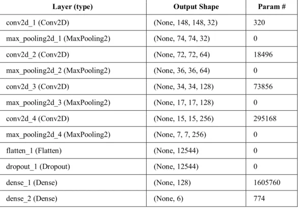
The second part after the flatten layer contains two dense layers for both approaches, but in full-color the first has 256 hidden units which makes the total number of network trainable parameters 3,601,478, in the other hand gray-scale approach has 128 hidden units in the fist dense layer and 1,994,374 as total trainable parameters, we shrank the size of the gray-scale network to avoid overfitting, for the last
layer for both has Softmax as activation and 6 outputs representing the 6 classes.
Table 1: Full-Color Model Summary.
Layer (type) Output Shape Param #
conv2d_1 (Conv2D) (None, 148, 148, 32) 896 max_pooling2d_1 (MaxPooling2) (None, 74, 74, 32) 0 conv2d_2 (Conv2D) (None, 72, 72, 64) 18496 max_pooling2d_2 (MaxPooling2) (None, 36, 36, 64) 0 conv2d_3 (Conv2D) (None, 34, 34, 128) 73856 max_pooling2d_3 (MaxPooling2) (None, 17, 17, 128) 0 conv2d_4 (Conv2D) (None, 15, 15, 256) 295168 max_pooling2d_4 (MaxPooling2) (None, 7, 7, 256) 0
flatten_1 (Flatten) (None, 12544) 0
dropout_1 (Dropout) (None, 12544) 0
dense_1 (Dense) (None, 256) 3211520
dense_2 (Dense) (None, 6) 1542
Table 2: Gray-Scale Model Summary.
Layer (type) Output Shape Param #
conv2d_1 (Conv2D) (None, 148, 148, 32) 320 max_pooling2d_1 (MaxPooling2) (None, 74, 74, 32) 0 conv2d_2 (Conv2D) (None, 72, 72, 64) 18496 max_pooling2d_2 (MaxPooling2) (None, 36, 36, 64) 0 conv2d_3 (Conv2D) (None, 34, 34, 128) 73856 max_pooling2d_3 (MaxPooling2) (None, 17, 17, 128) 0 conv2d_4 (Conv2D) (None, 15, 15, 256) 295168 max_pooling2d_4 (MaxPooling2) (None, 7, 7, 256) 0
flatten_1 (Flatten) (None, 12544) 0
dropout_1 (Dropout) (None, 12544) 0
dense_1 (Dense) (None, 128) 1605760
7.DATAVISUALISATION
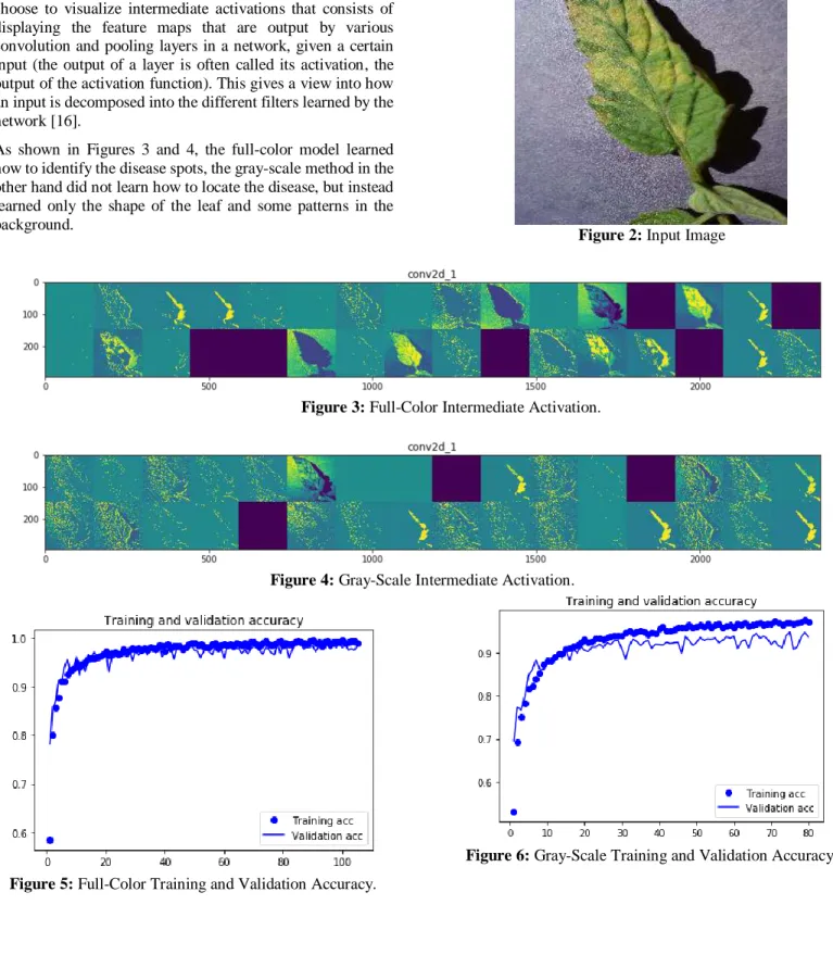
To see how the model works and what exactly learns we choose to visualize intermediate activations that consists of displaying the feature maps that are output by various convolution and pooling layers in a network, given a certain input (the output of a layer is often called its activation, the output of the activation function). This gives a view into how an input is decomposed into the different filters learned by the network [16].
As shown in Figures 3 and 4, the full-color model learned how to identify the disease spots, the gray-scale method in the other hand did not learn how to locate the disease, but instead learned only the shape of the leaf and some patterns in the background.
.
Figure 2: Input Image
Figure 3: Full-Color Intermediate Activation.
Figure 4: Gray-Scale Intermediate Activation.
Figure 5: Full-Color Training and Validation Accuracy.
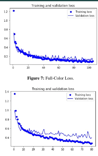
Figure 7: Full-Color Loss.
Figure 8: Gray-Scale Loss.
8.CONCLUSION
We are so proud to show that out best model (Full-Color) achieved an accuracy of 99.84% on a held-out test set, and second best model (Gray-Scale) achieved an accuracy of 95.54%, Figures 5 and 6 show how the models accuracy progress over epochs (as seen in Figure5-Figure8).
REFERENCES
1. A Survey of FPGA-based Accelerators for Convolutional Neural Networks", NCAA, 2018
2. Hussain, Mahbub; Bird, Jordan J.; Faria, Diego R. (September 2018). Advances in Computational Intelligence Systems (1st ed.). Nottingham, UK.: Springer. ISBN 978-3-319-97982-3. Retrieved 3 December 2018.
3. "CS231n Convolutional Neural Networks for Visual Recognition". cs231n.github.io. Retrieved 2017-04-25. 4. Grel, Tomasz (2017-02-28). "Region of interest pooling
explained". deepsense.io.
5. Krizhevsky, Alex; Sutskever, Ilya; Hinton, Geoffrey E. (2017-05-24). "ImageNet classification with deep convolutional neural networks" (PDF). Communications
of the ACM. 60 (6): 84–
90. doi:10.1145/3065386. ISSN 0001-0782.
6. Deshpande, Adit. "The 9 Deep Learning Papers You Need To Know About (Understanding CNNs Part 3)". adeshpande3.github.io. Retrieved 2018-12-04. 7. Dave Gershgorn (18 June 2018). "The inside story of
how AI got good enough to dominate Silicon Valley". Quartz. Retrieved 5 October 2018.
8. "The Face Detection Algorithm Set To Revolutionize Image Search". Technology Review. February 16, 2015. Retrieved 27 October 2017.
9. Huang, Jie; Zhou, Wengang; Zhang, Qilin; Li, Houqiang; Li, Weiping (2018). "Video-based Sign Language Recognition without Temporal Segmentation". arXiv:1801.10111 [cs.CV].
10. "Toronto startup has a faster way to discover effective medicines". The Globe and Mail. Retrieved 2015-11-09. 11. Maddison, Chris J.; Huang, Aja; Sutskever, Ilya; Silver,
David (2014). "Move Evaluation in Go Using Deep
Convolutional Neural
Networks". arXiv:1412.6564 [cs.LG].
12. Durjoy Sen Maitra; Ujjwal Bhattacharya; S.K. Parui, "CNN based common approach to handwritten character recognition of multiple scripts," in Document Analysis and Recognition (ICDAR), 2015 13th International Conference on, vol., no., pp.1021–1025, 23–26 Aug. 2015
13. "NIPS 2017". Interpretable ML Symposium. 2017-10-20. Retrieved 2018-09-12.
14. Zang, Jinliang; Wang, Le; Liu, Ziyi; Zhang, Qilin; Hua, Gang; Zheng, Nanning (2018). "Attention-Based Temporal Weighted Convolutional Neural Network for Action Recognition". IFIP Advances in Information and Communication Technology (PDF). Cham: Springer International Publishing. pp. 97–108. doi:10.1007/978-3-319-92007-8_9. ISBN 978-3-319-92006-1. ISSN 1868-4238.
15. Wang, Le; Zang, Jinliang; Zhang, Qilin; Niu, Zhenxing; Hua, Gang; Zheng, Nanning (2018-06-21). "Action Recognition by an Attention-Aware Temporal Weighted Convolutional Neural Network" (PDF). Sensors. MDPI AG. 18 (7): 1979. doi:10.3390/s18071979. ISSN 1424-8220
16. https://www.kaggle.com/emmarex/plantdisease, was retrieved 20/12/2018.
17. Al-Massri, R. Y., Al-Astel, Y., Ziadia, H., Mousa, D. K., & Abu-Naser, S. S. (2018). Classification Prediction of SBRCTs Cancers Using Artificial Neural Network. International Journal of Academic Engineering Research (IJAER), 2(11), 1-7.
18. Alghoul, A., Al Ajrami, S., Al Jarousha, G., Harb, G., & Abu-Naser, S. S. (2018). Email Classification Using Artificial Neural Network. International Journal of Academic Engineering Research (IJAER), 2(11), 8-14. 19. Metwally, N. F., AbuSharekh, E. K., & Abu-Naser, S. S.
Neural Network. International Journal of Academic Pedagogical Research (IJAPR), 2(11), 1-7.
20. Heriz, H. H., Salah, H. M., Abu Abdu, S. B., El Sbihi, M. M., & Abu-Naser, S. S. (2018). English Alphabet Prediction Using Artificial Neural Networks. International Journal of Academic Pedagogical Research (IJAPR), 2(11), 8-14.
21. El_Jerjawi, N. S., & Abu-Naser, S. S. (2018). Diabetes Prediction Using Artificial Neural Network. International Journal of Advanced Science and Technology,124, 1-10. 22. Abu Naser, S., Zaqout, I., Ghosh, M. A., Atallah, R., &
Alajrami, E. (2015). Predicting Student Performance Using Artificial Neural Network: in the Faculty of Engineering and Information Technology. International Journal of Hybrid Information Technology, 8(2), 221-228.
23. Elzamly, A., Abu Naser, S. S., Hussin, B., & Doheir, M. (2015). Predicting Software Analysis Process Risks Using Linear Stepwise Discriminant Analysis: Statistical Methods. Int. J. Adv. Inf. Sci. Technol, 38(38), 108-115. 24. Abu Naser, S. S. (2012). Predicting learners performance using artificial neural networks in linear programming intelligent tutoring system. International Journal of Artificial Intelligence & Applications, 3(2), 65.
25. Elzamly, A., Hussin, B., Abu Naser, S. S., Shibutani, T., & Doheir, M. (2017). Predicting Critical Cloud Computing Security Issues using Artificial Neural Network (ANNs) Algorithms in Banking Organizations. International Journal of Information Technology and Electrical Engineering, 6(2), 40-45.
26. Musleh, M. M., & Abu-Naser, S. S. (2018). Rule Based System for Diagnosing and Treating Potatoes Problems. International Journal of Academic Engineering Research (IJAER) 2 (8), 1-9.
27. Almadhoun, H., & Abu-Naser, S. (2017). Banana Knowledge Based System Diagnosis and Treatment. International Journal of Academic Pedagogical Research (IJAPR), 2(7), 1-11.
28. Abu-Nasser, B. S., & Abu-Naser, S. S. (2018). Cognitive System for Helping Farmers in Diagnosing Watermelon Diseases. International Journal of Academic Information Systems Research (IJAISR) 2 (7), 1-7. 29. Barhoom, A. M., & Abu-Naser, S. S. (2018). Black
Pepper Expert System. International Journal of Academic Information Systems Research, (IJAISR) 2 (8), 9-16.
30. AlZamily, J. Y., & Abu-Naser, S. S. (2018). A Cognitive System for Diagnosing Musa Acuminata Disorders. International Journal of Academic Information Systems Research, (IJAISR) 2 (8), 1-8.
31. Alajrami, M. A., & Abu-Naser, S. S. (2018). Onion Rule Based System for Disorders Diagnosis and Treatment. International Journal of Academic Pedagogical Research (IJAPR), 2 (8), 1-9.
32. Al-Shawwa, M., Al-Absi, A., Abu Hassanein, S., Abu Baraka, K., & Abu-Naser, S. S. (2018). Predicting
Temperature and Humidity in the Surrounding Environment Using Artificial Neural Network. International Journal of Academic Pedagogical Research (IJAPR), 2(9), 1-6.
33. Salah, M., Altalla, K., Salah, A., & Abu-Naser, S. S. (2018). Predicting Medical Expenses Using Artificial Neural Network. International Journal of Engineering and Information Systems (IJEAIS), 2(20), 11-17. 34. Marouf, A., & Abu-Naser, S. S. (2018). Predicting
Antibiotic Susceptibility Using Artificial Neural Network. International Journal of Academic Pedagogical Research (IJAPR), 2(10), 1-5.
35. Abu-Naser, S. S., Kashkash, K. A., & Fayyad, M. (2010). Developing an expert system for plant disease diagnosis. Journal of Artificial Intelligence, 3 (4), 269-276.
36. Jamala, M. N., & Abu-Naser, S. S. (2018). Predicting MPG for Automobile Using Artificial Neural Network Analysis. International Journal of Academic Information Systems Research (IJAISR), 2(10), 5-21.
37. Kashf, D. W. A., Okasha, A. N., Sahyoun, N. A., El-Rabi, R. E., & Abu-Naser, S. S. (2018). Predicting DNA Lung Cancer using Artificial Neural Network. International Journal of Academic Pedagogical Research (IJAPR), 2(10), 6-13.