FEATURE-BASED ANALYSIS OF OPEN SOURCE USING BIG DATA ANALYTICS
A THESIS IN Computer Science
Presented to the Faculty of the University Of Missouri-Kansas City in partial fulfillment
Of the requirements for the degree MASTER OF SCIENCE
By
MALATHY KRISHNAN
B.E, Anna University, 2012 Kansas City, Missouri
©2015
MALATHY KRISHNAN ALL RIGHTS RESERVED
iii
FEATURE-BASED ANALYSIS FOR OPEN SOURCE USING BIG DATA ANALYTICS Malathy Krishnan, Candidate for the Master of Science Degree
University of Missouri-Kansas City, 2015
ABSTRACT
The open source code base has increased enormously and hence understanding the functionality of the projects has become extremely difficult. The existing approaches of feature discovery that aim to identify functionality are typically semi-automatic and often require human intervention. In this thesis, an innovative framework is proposed for automatic discovery of features and the respective components for any open source project dynamically using Machine Learning. The overall goal of the approach is to create an automated and scalable model which produces accurate results.
The initial step is to extract the meta-data and perform pre-processing. The next step is to dynamically discover topics using Latent Dirichlet Allocation and to form components optimally using K-Means. The final step is to discover the features implemented in the components using Term Frequency - Inverse Document Frequency algorithm. This framework is implemented in Spark that is a fast and parallel processing engine for big data analytics. ArchStudio tool is used to visualize the features to class mapping functionality. As a case study, Apache Solr and Apache Hadoop HDFS are used to illustrate the automatic discovery of components and features. We demonstrated the scalabilty and the accuracy of our proposed model compared with a manual evaluation by software architecture experts as a baseline. The accuracy is 85% when compared with the manual evaluation of Apache Solr. In
iv
addition, many new features were discovered for both the case studies through the automated framework.
v
APPROVAL PAGE
The faculty listed below, appointed by the Dean of the School of Computing and Engineering, have examined a thesis titled “Feature-based Analysis for Open Source using Big Data Analytics” presented by Malathy Krishnan, candidate for the Master of Science degree, and hereby certify that in their opinion, it is worthy of acceptance.
Supervisory Committee
Yugyung Lee, Ph.D., Committee Chair School of Computing and Engineering
Yongjie Zheng, Ph.D., Committee Co-Chair School of Computing and Engineering
Praveen Rao, Ph.D.
vi TABLE OF CONTENTS ABSTRACT ... iii ILLUSTRATIONS ... viii TABLES ...x Chapter 1. INTRODUCTION ...1 1.1 Overview ...1 1.2 Motivation ...1 1.3 Problem Statement ...3 1.4 Proposed Solution ...3
2. BACKGROUND AND RELATED WORK ...6
2.1 Overview ...6
2.2 Terminology and Technology ...6
2.3 Related Work ...10
3. FRAMEWORK OF FEATURE-BASED ANALYSIS ...14
3.1 Overview ...14 3.2 Framework ...14 3.2.1 Meta-data Extraction ...15 3.2.2 Component Identification ...19 3.2.3 Feature Discovery ...21 3.2.4 Visulazation ...22
4. COMPONENT IDENTIFICATION AND FEATURE DISCOVERY ...25
vii
4.2 Camel Case Split ...25
4.3 Topic Discovery ...25 4.4 Component Identification ...30 4.5 Feature Discovery ...33 5. IMPLEMENTATION ...37 5.1 Overview ...37 5.2 Meta-data Generation ...37 5.3 Component Identification ...41 5.4 Feature Discovery ...45
6. RESULTS AND EVALUATION...47
6.1 Overview ...47
6.2 Accuracy ...47
6.3 Evaluation of Optimization ...55
6.4 Verification ...59
6.5 Results ...63
7. CONCLUSION AND FUTURE WORK ...73
7.1 Overview ...73 7.2 Conclusion ...73 7.3 Limitation ...74 7.4 Future Work ...74 REFERENCES ...75 VITA ...77
viii
ILLUSTRATIONS
Figure Page
1: Workflow of Proposed Solution ...15
2: Meta-data Extraction Phase ...16
3: Kabbalah Model ...17
4: Steps in Component Identification ...21
5: Discovered Features in Components ...22
6: Architecture Diagram in ArchStudio ...23
7: Feature List With Variants in ArchStudio ...23
8: Example Illustrating Word Count ...26
9: Flow of LDA ...29
10: Flow of K-Means ...32
11: HeatMap for K-Means data ...32
12: Flow of TF-IDF ...34
13: Hybrid Approach ...36
14: Intermediate HashMap ...39
15: Example Illustrating LDA ...42
16: Example Illustrating K-Means ...44
17: Example Illustrating TF-IDF ...46
18: Apache Solr Statistics ...48
19: Number of Feature and Feature Variants in Apache Solr ...50
ix
21: Feature and Feature Variants Accuracy ...52
22: Precision and Recall...53
23: Newly Discovered Features ...55
24: Automated Identification of Topic Number in LDA ...56
25: Graph for Finding ‘K’ in K-Means ...57
26: Feature Comparison ...57
27: Accuracy Comparison...58
28: Runtime Performance ...58
29: Parallel Processing Results for Apache Solr...59
30: Comparison of Clusters for Apache Solr ...60
31: Comparison of Clusters of Apache Solr ...60
32: Hadoop HDFS Statistics ...61
33: Cluster Comparison for Hadoop HDFS ...62
34: Overall Comparison for Hadoop HDFS Components ...63
x TABLES
Table Page
1: Statistics of Open Source Repositories ...1
2: Objectives and Limitation of Related Work ...12
3: Example of Kababalah Model ...38
4: Conversion from RDF to Intermediate Hashmap ...40
5: Transition from LDA Output to K-Means Input ...42
6: Solr Statistics Generated by Rdfcoder ...48
7: Confusion Matrix for Precision and Recall ...54
8: Number of Clusters in Two Approaches ...61
9: Solr Statistics Generated by RDFCoder ...62
10: Feature and Feature Variable Statistics for Hadoop HDFS ...63
11: Topic Distribution for Classes ...64
12: Classes in a Sample Set of Cluster...65
13: Features in Approach 1 ...66
14: Features in Approach 2 ...68
15: Comparison of Features from Manual and Automated Analysis ...69
1 CHAPTER 1 INTRODUCTION
1.1 Overview
This chapter describes about the existing problem and the motivation for the research in section 1.2. The next section 1.3 gives the problem statement and section 1.4 describes the proposed solution for the problem statement. This chapter gives the high level introduction for the thesis research.
1.2 Motivation
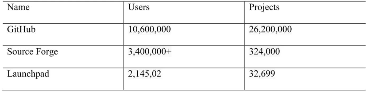
As the open source code repositories are increasing day by day, there are a lot of good quality source code which is available. The repositories, projects, users in open source area are predominantly increasing. Table 1 shows the number of users and projects [10] in few of the open source projects. The open source has been there for the past two decades, but there is an increase in the involvement of people and companies for open source in the current decade. Open source is one of the main places to search for projects which can be reused. As the number of software developers is increasing day by day, the tactic is how to be smart in writing code by reusing the existing code and getting things done in a short period of time.
Table 1: Statistics of open source repositories.
Name Users Projects
GitHub 10,600,000 26,200,000
Source Forge 3,400,000+ 324,000
2
Having code written in open source is becoming a more common process and a standard across software developers, who are developing projects in open source. And as a developer, understanding and reusing a code base is very important. With that said, maintaining a set of rules and guidelines for an open source code base will result in a reusable code base and a high quality project.
As analyzing and understanding the code written by others is not a simple task, the software developer’s assumption is that writing code for the requirement is better than analyzing the existing code. Lack of analytical tools is the reason behind this. Even though the software developers want to re-use the code, the time taken to analyze the code is much more than writing new code. Another harder task is to find the part of the project that has the functionality which the software developer is looking for. If the selected open source is a huge project, the software developer needs to spend a lot of time to identify the module in which the code is written. As the open source code base is huge, the same functionality can be implemented in multiple different projects and hence gets harder for the developer to identify and analyze the different code base. In certain cases the code is too complex because it has a lot of files, packages and classes hence making it even harder to navigate between different packages to understand the code.
Manually analyzing the project is a tedious process and it does not guarantee the accuracy and there might be problems capturing the internal details of the class, if the developer just uses the documentation to understand about the project. In certain cases when there are no good documents, the developer has to read through the code to understand which is very difficult. All these factors discourages the programmers to reuse the high quality open source code base. Finding the functionality and the code which implements the functionality in the
3
project is one of the best ways to reuse the existing code. Feature can be defined as the functionalities implemented in the code base. The components are a group of classes which implements the feature. The automatic feature analysis tool presented in this thesis uses machine learning techniques and big data analytics to completely automate the feature and component discovery. It has various applications that would be very useful for the software developers and end users.
1.3 Problem Statement
The open source repositories has increased vastly. With this the developers have working high quality code available for them to reuse. But analyzing the source code might be time consuming as the code is huge. The open source projects either have no documentation or the documentations are too long for the user to read and understand. Hence, understanding the functionality of each project becomes extremely difficult. The existing approaches of feature identification are semi-automatic and often require human intervention. Manually identifying the features for all open source projects is practically not possible. Our research is a semantic approach to automatically discover the features and identify the components based on feature similarity of classes from a given code base. The goal of the approach is to create an automated and scalable model which produces accurate results.
1.4 Proposed Solution
In our research, a big data analytics model is proposed for automatic discovery of components and features for open source projects using Machine Learning. Open source code base is huge and semi/unstructured. Hence, big data analytics is required for analysis and
4
processing. Feature discovery can be defined as the functionalities implemented in the code base. The components are identified based on the implementation of features. Machine learning is an ongoing process with which the model can become more intelligent as it learns from different code bases. The above explains why we chose on open source projects and big data analytics.
This research focuses on the problem of recovering the features of open source projects. Many of the current applications that are being developed are not novel in its entirety, hence reusing the source code will help in the software development process. Since there are no proven techniques to analyze source code, the feature discovery and reusability is an important problem in software development. The idea here is to get the meta-data from the source code and use machine learning techniques to analyze the meta-data and get some meaningful information which would be helpful in identifying the components and discovering the features of the selected code base.
The initial step is to extract the meta-data and perform pre-processing. The next step is to dynamically discover topics using Latent Dirichlet Allocation and to form components optimally using K-Means. The final step is to discover the features implemented in the components using Term Frequency - Inverse Document Frequency algorithm. This framework is implemented in Spark that is a fast and parallel processing engine for big data analytics. ArchStudio tool is used to visualize the features to class mapping functionality. As a case study, Apache Solr and Apache Hadoop HDFS are used to illustrate the automatic discovery of components and features. We demonstrated the scalabilty and the accuracy of our proposed model compared with a manual evaluation by software architecture experts as a
5
baseline. Thus, for a given a code base, the entire model results in a list of components grouped by feature similarity of classes and the feature list of each component.
6 CHAPTER 2
BACKGROUND AND RELATED WORK 2.1 Overview
In this chapter we will define the terms that have been used throughout the thesis and also introduce the technologies in section 2.2. We will also discuss the problems with other approaches proposed for architecture recovery and the related work in section 2.3.
2.2 Terminology and Technology
In this section we will define the terms that have been used throughout the research and also introduce the technologies used. The software architecture [18] is the top most level of a software system. It comprises a set of elements which gives more meaning to the software system. These elements have relations between them with which they interact. The underlying software system contains a list of principle design decisions. Various functionality components and their relationship comprises the architecture of a software system. A code entity is a programming entity, since our research focuses on Java projects, the main code entities are methods, classes, packages, interfaces, etc. A component is a set of classes which implements one or more functionality. A feature is a functionality of the project. Feature Vector used in the context of machine learning represents data object which are used by machine learning algorithms.
RDFCoder [11] is an open source project which helps in the conversion of Java code to a
meta-data file in RDF format. A jar is a native library used by applications on Java platform. It is a package format which aggregates many Java class files and associated meta-data and resources into one file. RDFCoder takes a JAR (a package file including Java class files and
7
associated meta-data and resources) or a source code for the conversion. It can be used in command line or as a library in a Java project. It analyses the structure of the source code through packages, classes, methods, attributes and gives the relationship between them. The main elements of RDFCoder are:
Java Source Parser - a set of classes able to parse java files and convert its contents in Code Handler events.
Java Bytecode Parser - a set of classes able to parse .class files (eventually inside .jar archives) and convert its contents in code handler events.
Javadoc Parser - a set of classes able to parse .java files Javadoc documentation and
convert it in Code Handler events.
Code Handler - the code handler is a class able to convert class events in RDF triples.
The way the Code handler translates received events into triples is described
in model section. Despite the code handler currently generates only RDF triples, in theory this can generate any entity representation compliant with the interface of the Code Model.
Objects Table - the Code Handler needs to fully qualify (i.e., add full package
qualification) all the objects it finds during the compilation process.
The fully qualification is done by populating and querying the Objects Table. Every time that an object needs to be fully qualified, the Objects Table is inquired by providing the object name and the Imports Context that is the list of the imports provided when used the object itself.
Code Model - the Code Model is a container of the triples representing a bunch of related libraries. A code model provides operations to add triples, remove triples, and perform basic search and complex queries on triples.
8
may rely on any support able to store relationships among the entities involved in the code representation.
Code Storage - the Code Storage is a set of classes meant to make persistent a code
model. There may be several persistent storages like file system or a RDMS.
Query Engine - the Query Engine is a set of classes meant to perform queries on storage. At the moment the only supported query language is SPARQL.
Model Inspector - the Model Inspector is a high level representation of the Code Model. By using the Model Inspector it is possible to navigate Java objects representing the entities stored into the model.
RDFCoder uses the Kabbalah model [11] is the ontology for representing code entities which defines resources and relationships among them. Every resource that are within the model is an Identifier. A resource identifier represents every resource in that model.
Resource Description Framework [13]: It is known as RDF in short form. This model is the web
standard for interchange of data. To name the connection or the relationship between things RDF uses URIs which is used as linking structure of the web. “Subject-predicate-object” expressions are used in RDF.
1. Triple: The “subject-predicate-object” expression is called as Triple. 2. Subject: Resource is denoted as subject.
3. Predicate: A predicate shows aspects or traits of the resource. It denotes a relationship or connection between subjects and objects.
9
SPARQL: SPARQL [17] is query language for RDF which helps to manipulate and get the data which are stored in RDF format. There are different query variations in SPARQL language which can be used for various purposes. Few of the useful query patterns are listed below with explanation:
SELECT query helps to retrieve raw values from a given SPARQL query.
CONSTRUCT query is used to transform the result to a table after extracting information from the SPARQL endpoint.
ASK query is used to give a True/False value for any given SPARQL query.
DESCRIBE query is used to provide an graph form of RDF from the SPARQL endpoint, the contents of that is based on the endpoint to decide whether the maintainer considers as useful information.
Feature is any functionality that is implemented in the project. Feature Variant is a variant from the primary feature. We have not considered options like optional or compulsory that are typically described in Product Line Architectures. The feature variants are extracted from the project and hence only implemented variants are extracted. Components are a set of classes in which the feature is implemented. It is not a high-level architecture component like frontend or user interface. It is more specific to the features implemented.
Machine Learning Clustering [20]helps to group similar entities together based on the
similarity. To identify the similar classes, a feature vector has to be generated explaining more about the class in terms of its numbers. Hence in this approach, the percentage of topics in each class is the feature vector matrix generated by Latent Dirichlet Allocation. Clustering assigns a cluster number to all the similar classes that are grouped together based on their similarity.
K-10
Means is one of the best algorithms which is used for clustering [23]. Term Frequency – Inverse Document Frequency is a statistical algorithm used to find the top words in each components which are the features in each component.
2.3 Related Work
There is a rapid growth in the feature based analysis research. Automating the entire process in feature based analysis is difficult. The general practice of recovering is with the domain knowledge. In case of domain knowledge, the person who developed the system or who knows the project needs to give some input. In case of open source projects, when there are more than thousands, getting input from the developers is a difficult and time consuming process. Garcia and Mattmann [1] state that it is necessary to have the ground truth information about the project from the developers to recover the architecture. More information about the project is required for mapping the components and to refine the architecture. In our approach, we overcome this by analyzing the code base and getting more details from the class, package and other details. Hence, these details are used for the feature based analysis and component identification. Most of the research have domain knowledge as a base for architecture recovery, but the proposed model is completely automated and no information is required from domain experts for analysis. Marx and Beck [3] discuss about extracting the components in a software project. Their main aim is to identify the feature implemented in a set of classes and group them as a component. They try to minimize the interactions between components and hence, reuse of the feature can be done easily by using the component as the interaction with other components are minimum. The main disadvantage of this process is that if there are many dependencies, this approach might not give good results. But in the proposed model, dependencies does not matter,
11
since the details are taken from the code base and the dependencies do not play a role on the analysis for the architecture recovery. Dit and Revelle [2] analyzed 25 different articles in feature based analysis. The analysis is from 3 different aspects, which are manual feature analysis, tool based analysis and domain expert analysis. Manual analysis was time consuming and the results were not consistent as different people have different perspectives. There were few tools which were developed to analyze the feature. But they required domain knowledge to a certain extent for analysis. The domain knowledge was another approach where experts who developed the project or who know the project give some information about the architecture and feature which is then used for the analysis. In all these cases, there was no standard way to verify the results. But in our proposed model, the entire process is completely automated and hence no domain knowledge or manual intervention is required. The results are compared with the manual analysis done by a group of software architect experts who analyzed the Apache Solr code base. Table 2 gives a high level comparison between three papers.
12
Table 2: Objectives and limitations of related work
Hitesh and Cristina [9] proposed a model for automatic architecture recovery using one classification of machine learning algorithms which is unsupervised. To represent the dynamic, lexical and static aspect of the software, this approach uses three different feature sets that is similar to the approach used in this thesis. From the source code, the information used for the static features is extracted. It also involves method invocations by code entity, inheritance relationships among classes and user defined access. From the definition of method, the method names, packages, variables, parameters, closing types, etc., the lexical features are derived, which capture the domain information. The dynamic features involves the method call frequency. For the recovery of the components in the software system architecture, this model combines and compares the dynamic, lexical and static features mentioned. The clustering is done based on methods that have been denoted by a features vector and the classes are clustered
13
depending on the similarities they have. Because of the fact that there could be generic method names, their clustering technique might not result in the correct component sets. Koschke [19] explained about the component architecture recovery in the thesis. In the approach the model is semi-automatic and hence need human interaction in certain steps to identify the components. The comparison also required software engineer experts to verify the results. The model proposed in this thesis is completely automatic and hence no manual intervention is required in any of the steps.
14 CHAPTER 3
FRAMEWORK OF FEATURE-BASED ANALYSIS 3.1 Overview
The thesis proposes a framework which aids in component identification and feature discovery. The overview of the framework is explained in section 3.2 and the various different parts of the framework are explained in the future sections. Meta-data extraction is explained in section 3.2.1. Component identification and feature extraction is explained in section 3.2.2 and section 3.2.3 respectively. The environment used is Spark which is a scalable platform. The last section 3.2.4 is the visualization where the tool ArchStudio is used.
3.2 Framework
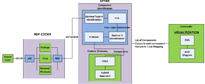
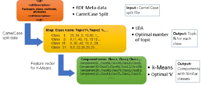
The framework that aids in component identification and feature discovery consists of three components. The first is the meta-data extraction, second in the flow implemented in Spark environment and the third is visualization. The initial step is to parse the given source code with RDFCoder to get the meta-data. This meta-data is then parsed to extract useful information like the class names, attributes, method, parameters, return type and packages. This data is then sent to LDA (Latent Dirichlet Allocation) which gives more information on grouping the classes together based on similar topics(features).The output from LDA is sent to K-Means clustering algorithm, where similar classes are grouped together based on the topic discovery, to form different components. Each component with the details of the classes is then sent to TF-IDF to discover their functionality. The above machine learning algorithms are implemented in Spark, Scala and Java. Thus, for a given a code base, the entire model results in a list of components grouped by similarity of classes and the feature list of each component.
15
The entire flow of the proposed model is illustrated in Figure 1. The input to the application is source code which can be source jar file. The RDFCoder gets the meta-data from the source code. This is the pre-processing step. The next step is the component identification and feature discovery which is executed in the Spark environment. The final step is the visualization to give more details of the input source code.
Figure 1: Workflow of proposed solution
The major components of the model include pre-processing using RDF Coder, component identification and feature extraction in spark environment and visualization which are discussed in detail in the later sections. The entire process is automated and hence no manual intervention is required. If the user gives the input source code for the feature extraction, the process is completely automated and the final features of the source code is discovered. The overview of each component is explained in the section below.
3.2.1 Meta-data Extraction
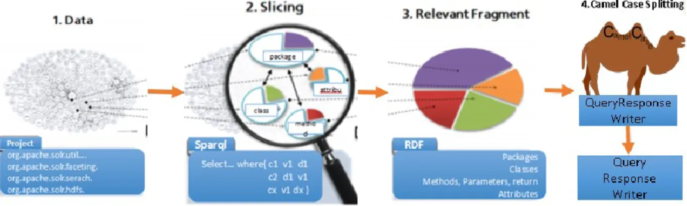
The input to the system which is also the input to the meta-data extraction stage is the Java project source. The meta-data, a RDF representation of the code base, is then used by
16
component identification and feature discovery to identify important information from meta-data which rules the functionality of the source code. This meta-data is also utilized during few of the machine learning algorithms to generate a recurring list of keywords in the project which determines the functionality of the project. Meta-data generation is the first step where the whole code of the Java project is converted into its RDF representation. This representation majorly contains the meta-data for all the code entities in the project like package, interface, class, attributes, and methods while retaining the code structure. The meta-data was generated as an RDF document in RDF format which was then parsed to extract the relevant features discussed in the following sections. The Java Compile Time Annotations API can also be used to extract annotation information which was not available through RDFCoder. The library information can also be extracted along with the class details to get more information about the source code. Figure 2 give a visual representation of meta-data.
Figure 2: Meta-data extraction phase
Binkley [7] explains the source code analysis as a method in which the code is automatically consumed from its code base or an artifact which is from the code base. Three main components are identified: the internal representation, the parser and the representation of this analysis. Binkley [7] use an RDFizer as the semantic data model as the internal
17
representation, the parser and SPARQL query as the component analysis. This meta-data gives information about the organization of classes, interfaces, methods etc. within the various packages present in the project package.
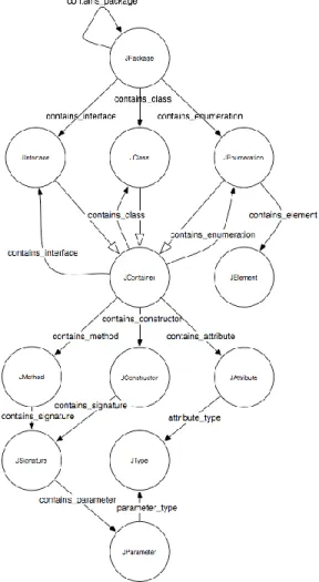
The Kabbalah model is the ontology used by RDFCoder. It defines resources and relationships among resources. The resources are every element in the source code. All the elements are uniquely identifies. Figure 3 is the model. RDFCoder is an open source project and seems to be one of the best way to extract the meta-data from a given code base. The identifiers have a fixed structure that can be represented with the following BNF rules:
18 <IDENTIFIER> ::= (<PREFIX> '#')? <SECTIONS>; <SECTIONS> ::= <SECTIONS> '.' <SECTION> | <SECTION>; <SECTION> ::= (qualifier ':')? Fragment;
All identifier can have a prefix that must end with '#'. The identifier contains a sequence of different sections separated by '.', every section must define a fragment and may contain a qualifier. The characters '#' '.' ':' are used to indicate the different parts of the identifier, for this reason they cannot be used neither in the qualifiers or fragments nor in the prefix. The meta-data has the certain useful information extracted from the source code. The key features are the code entities which are determining the nature or behavior of class. The following identifies the functionality of the class in Java, through the code entities.
1) Class
2) Package which has the class 3) Parent class
4) Methods contained of the Class 5) Member variables in the Class
6) Type of parameters the constructor accepts 7) Type of parameters the method accepts
The meta-data from RDFCoder is parsed to get more useful information. Details such as class, package, method, attribute, parameter and return types are identified from the meta-data. These details will be used in the approach to identify components and discover features.
19
3.2.2 Component Identification
The framework in which component identification and feature extraction are implemented is Spark. Spark [12] is a good environment for in-memory and iterative computing. The major advantage is it provides caching intermediate data in-memory for better access times. Real time querying of data, stream processing, sensor data processing are few of the use cases of spark where the performance is better than Hadoop. Similarly Spark can run the same Map Reduce jobs, with the difference being, it first places the data into RDDs [16] (Resilient Distributed Datasets) so that this data is now cached in-memory so it is readily accessible. Since it is in-memory processing, the same MapReduce jobs can run quickly. There is also flexibility to write queries in Scala, Java and Python. Spark is an Apache project advertised as “lightning fast cluster computing”. It has an enormous audience in open source community and is the most sought after Apache project. Spark provides a faster and more general data processing platform. It makes it possible to write code more faster as it has more than 80 high-level operators at it is disposal. It also has the flexibility to run programs up to 100 times faster in memory, or 10 times faster on disk, than Hadoop.
In the component identification, similar classes are grouped together to form the component. Two different algorithms are used to get the best result in this step. The meta-data from previous step is further processed to get the class and the related words in each class as a single line. All the multi gram words are split using camel case. This intermediate data is then fed to Latent Dirichlet Allocation algorithm where topics in each class are discovered. LDA was first presented as a graphical model and its main focus is topic discovery.
In Latent Dirichlet allocation (LDA) is a topic discovery model. This is one of the best
algorithm to identify the hidden topics in a given context. It is a probabilistic model and hence more accurate results are analyzed. This model explains certain unobserved groups with a set of
20
observable to show why certain parts are similar. This algorithm gives the percentage of each topic in a given document and hence it is easier to analyze the relationship between classes
The resultant topics are converted to percentage of topic for all the classes. The input for K-Means algorithm is the class name and the percentage of each topic in the form of matrix. In
K-Means Clustering technique, K centroids are randomly initialized in the data. The K is decided
by the dataset and hence the entire process is automated. The algorithm loops through the data in the dataset, which is assigned to the closest centroid in the pool. After each loop, the recalculation of the centroid occurs and it is repeated until convergence. The threshold error or the constant cluster assignment is called convergence. K-Means is one the best algorithm for clustering owing to its simplicity.
Certain input parameters have to be supplied to K-Means algorithm to get accurate results. Since, K-Means is a parameterized hence the results are highly reactive to the parameter values. Finding the number of clusters is an important parameter in the algorithm and hence more importance should be given to it. Since this is unsupervised learning and the end user does not know anything about the project, it is not a good practice to get the input parameter from the end-user regarding the cluster number size. Hence, Sum of Squared Errors method is used to determine the number of clusters. The best value of K is determined by Sum of Squared Error analysis which plots the sum of distance of every data points from its respective cluster centroids against configurations of different cluster. As the cluster number is increasing the cost decreases and it gets stagnant or there is very less decrease in the cost. This determines the number of clusters in K-Means algorithm. Hence, the process to find the value of ‘k’ is automated. The result is the cluster with a set of similar classes grouped together. Figure 4 gives steps in component identification.
21
Figure 4: Steps in component identification
3.2.3 Feature Discovery
Feature discovery is the next step after component identification. As similar classes are grouped together, finding the features in each component is the next step. The most important feature can be found in each component using TF-IDF which id Term Frequency - Inverse Document Frequency to identify the significant keywords in the components. Term Frequency Inverse Document Frequency (TF-IDF) computes the weights that indicate the importance of words in the corpus. This algorithm is used as a weighting factor which is used to compute the numerical statistic for the words in the corpus. This algorithm is often used in text mining to find the important words and hence identify the topic of the document or the corpus. The TF-IDF algorithm not only analyses the frequency, it has an inverse proportion with the corpus. Hence, even if a term is repeated many times in a document, its weight will be decreased so that it may not be considered as an important term.
TF-IDF has been used in place of a regular frequency count to get rid of terms which appear in many classes since they do not hold a high significance. The top keywords with high
22
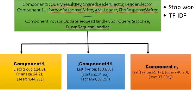
TF-IDF score are then identified. This gives the functionality of each component. Form the split camel case words, the full words are traced back to get the complete meaning of the word used in the component. Figure 5 shows the discovered features in each cluster.
Figure 5: Discovered features in components
3.2.4 Visualization
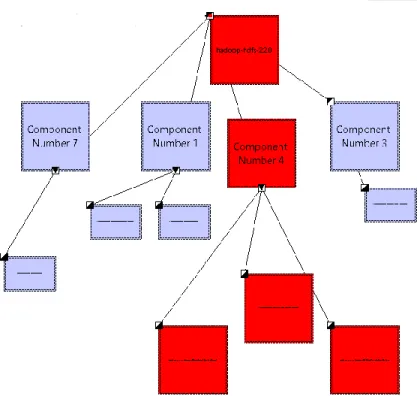
Once the features of identified, the important part is visualization, as this helps the user to easily understand about the project. Highcharts [21] and Graphs can be used to visualize the number of components and features in the project. Protégé can also be used to get more details in terms of ontology. ArchStudio is a tool to visualize software architectures. The XML file can be built from the result of the proposed model and this file can be visualized in Eclipse’s ArchStudio plug-in. Figure 6 show the architecture diagram and Figure 7 shows the sample feature list of Solr Code.
23
Figure 6: Architecture Diagram in ArchStudio
24
The main project is the highest level component and there are many sub components which are composed of multiple classes. For example, component 4 has 3 classes that are the NativeIO, LayoutVersion, VersionMismatch. Similarly there are various feature for the project and certain feature and feature variants are listed in the above figure.
25 CHAPTER 4
COMPONENT IDENTIFICATION AND FEATURE DISOVERY 4.1Overview
This chapter gives the complete flow for component identification and feature discovery. Section 4.2 is the first step after meta-data generation which is camel case split. Section 4.3 and 4.4 describe about topic discovery and component identification. Feature discovery is explained in section 4.3.
4.2Camel Case Split
The meta-data from RDFCoder is split using camel case mechanism. Camel casing means capitalizing the first word in a phrase of words. This mechanism is used in most of the programming language. This is the commonly followed standard in Java programming. For example, PythonWriter will be split as python and writer. Camel case splitting is necessary because the compound words could not be properly recognized during the analysis. More meaning is given to the phrase of words only when it is split. For example, Write might have different types like PythonWriter, RubyWriter, PhpWriter, etc. If there are complete phrase of words, it will be hard for the machine to understand that all these fall under the feature writer. Substring match might not be good, as some words contain many other words between them.
4.3Topic Discovery
The input to the word count program is an intermediate file which has the class name as the first word followed by a tab space and a list of words. The list of words are from the meta-data which are split by Camel case. Word Count Algorithm is used to count the number of same
26
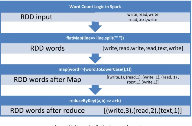
words in a given document. In our approach, one single file is the input and each line in a file is considered as a document. Map Reduce in Spark environment is used to execute word count. Figure 8 is an example illustrating word count.
Figure 8: Example illustrating word count
Latent Dirichlet allocation (LDA) is a topic discovery model. This is one of the best
algorithm to identify the hidden topics in a given context. It is a probabilistic model and hence more accurate results are analyzed. This model explains certain unobserved groups with a set of observable to show why certain parts are similar. This algorithm gives the percentage of each topic in a given document and hence it is easier to analyze the relationship between classes. LDA was first presented as a graphical model and its main focus is topic discovery.
In LDA, each document has a set of topics which are identified by the algorithm. This resembles a probabilistic latent semantic analysis known as pLSA, the exception is that the distribution of topic is assumed to have a Dirichlet prior in LDA. Since we get a list of topics
reduceByKey((a,b) => a+b)
RDD words after reduce
[(write,3),(read,2),(text,1)]
map(word=>(word.toLowerCase(),1))RDD words after Map
[(write,1), (read,1), (write, 1), (read, 1) , (text,1),(write,1)] flatMap(line=> line.split('" "))RDD words
[write,read,write,read,text,write]
Word Count Logic in Spark27
for a given document the approach used in LDA seems more reasonable. For example, the topics in a LDA model can be classified as database-related and writer-related. The database-related words like their columns, fields, table, and query will be classified as database-related. But the word database will have higher probability for the topic. Similarly, all the writer-related words like python writer, ruby writer, file, text, etc. will be classified as writer-related. IF there are certain words that are used by both of the topics, it will have an equal probability distribution. This topic discovery model is based on probability and likelihood. A lexical word analyzer identifies the words and assigns the probability or the word to be related to the topic. Hence, from the above method, each document has a list of topics identified. A particular topic set characterizes every document in the given list.
LDA is a topic model used for identifying the topics in each class. The input to the LDA model is a word document with a class name followed by a tab space and all the semantics related to the class (split method names, attribute names, etc.).
28 LDA Pseudocode:
1. Collect the words from file 2. Term count
3. Stop words, if any
4. Create Map(Word, count) 5. Generate LDA model 6. Calculate current_likelihood
7. While ( current_likelihood < previous_likelihood) Regenrate LDA model
Recalculate current_likelihood Exit condition: Model = previous_model Likelihood = previous_likelihood 8. End while Steps in LDA:
Following are the steps implemented to infer the topics/features based on the semantics in the classes.
1. Word count: Each class is considered as a document. First we calculate the word count based on the information in all the documents.
2. Stop Words: We need to eliminate the mostly commonly occurring words like the, get, set.
3. Important words: After eliminating the stop words, we determine the most important words based on the word count.
4. LDA Model: For each class, the word count is computed for the important words and a word vector is built. The input to the LDA is a matrix of word vectors. Each row
represents the word counts for a particular class. The LDA model infers topics and gives the probabilities of each word in the topic.
29 The parameters for LDA are:
1. Number of important words 2. Number of topics
3. Number of words in each topic Optimal topic number identification:
For better results, we need to determine the above mentioned parameters. The algorithm is made optimal by selecting the optimal value for number of terms. Hence, for any given project, the number of topics will be selected according to the loglikehood that is the probability of the word belonging to a given topic. Finding the log likelihood helps in determining the number of topics. Following figure 9 explains the flow of LDA.
30
4.4 Component Identification
In K-Means Clustering technique, K centroids are randomly initialized in the data. The
K is decided by the dataset and hence the entire process is automated. The algorithm loops through the data in the dataset, which is assigned to the closest centroid in the pool. After each loop, the recalculation of the centroid occurs and it is repeated until convergence. The threshold error or the constant cluster assignment is called convergence. K-Means is one the best algorithm for clustering owing to its simplicity. This clustering algorithm is parametrized and hence choosing the correct value for the parameter is important. The K determining step is important in getting optimal results from the K-Means clustering algorithm. Instead of getting the number of clusters from the user, we can automate the process of identifying the correct K, using Sum of Squared Errors. Sum of Squared Errors method is one of the best ways to identify the number of clusters for a given data set.
K-Means is a clustering algorithm. After determining the percentages of topics in each class, we need to cluster the classes with similar topics. K-Means is used for this purpose. The input to the K-Means algorithm is a matrix where all the values are double. Once this input is given to K-Means, Sum of Squared Errors method is implemented to calculate the best value of K for the given cluster. The seed value is one of the hyper parameters used to incorporate randomness into the training data. The result of the K-Means are the classes clustered together. Similar classes are clustered together according to the input matrix. The following is the pseudocode of K-Means.
31 K-Means Pseudocode:
1. Collect the data from file
2. Filter the double values and class from feature vector 3. Create a Map(class, double values)
4. Generate K-Means model 5. Find the Sum of Squared Errors
6. While (Minimal Difference between Sum of Squared Errors) Regenerate K-Means model
Exit condition:
Select the model for K-Means 7. End While
Steps in optimal K-Means:
1. Feature vector: Find the feature vector with the output of LDA.
2. Find optimum ‘k’: For any given project, select the optimal number of cluster. 3. K-Means model: Create a K-Means model.
Optimal cluster number identification:
Dynamic identification of the number of cluster makes the model optimal for any given project. It is very important to select the correct parameter for K-Means, especially the number of clusters. Sum of Squared Errors method is used for identifying the number of clusters in K-Means. To identify the number of clusters in K-Means algorithm, Sum of Squared Errors method is used. The automated approach follows the steps in which the cost of computing K-Means is calculated for each cluster. It is an iterative process to calculate the cost by increasing the cluster number. Once the difference between the costs of consecutive cluster number becomes stagnant, that cluster number is identified. This determines the number of clusters in K-Means algorithm. Figure 10 explains diagrammatically the flow of K-Means and figure 11 gives the HeatMap for K-Means data set.
32
Figure 10: Flow of K-Means
The output of LDA is converted to the following format before giving it to K-Means. Each line has a class name followed by the percentage values for the topics delimited by comma.
33
Figure 9 shows the HeatMap with the K-Means data. HeatMap is generated using certain RStudio[14] libraries.
4.5 Feature Discovery
Feature is any functionality that is implemented in the project. Feature Variant is a variant from the primary feature. It does not have options like optional or compulsory. The feature variants are extracted from the project and hence only implemented variants are extracted. The feature and feature variants are discovered using TF-IDF.
Term Frequency Inverse Document Frequency (TF-IDF) computes the weights that indicate the importance of words in the corpus. This algorithm is used as a weighting factor which is used to compute the numerical statistic for the words in the corpus. This algorithm is often used in text mining to find the important words and hence identify the topic of the document or the corpus. The TF-IDF algorithm not only analyses the frequency, it has an inverse proportion with the corpus. Hence, even if a term is repeated many times in a document, its weight will be decreased so that it may not be considered as an important term. The input is an intermediate file which has the class name as the first word in the line and followed by a tab space and a list of words form the meta-data which is split by Camel case and spaced with a single space.
TF-IDF is the product of two statistics, term frequency and inverse document frequency. The value of term frequency in each document is calculated and the other metric is the inverse document frequency. The formula for each of the metric is explained below. The tern frequency is the frequency of the term appearing in the document.
34
TF(t,d) is the number of times that term t appears in document d Document frequency is the frequency of the document that contains the term.
DF(t,D) is the number of documents that contains term t
The document frequency has to be inverted to get the inverse document frequency. Hence, the log of document frequency and the below formula is applied.
IDF(t,D)= log|D|+1 DF(t,D)+1
The final step is to multiply the document and inverse document frequency to get the importance of the term in the cluster.
TFIDF(t,d,D)=TF(t,d) * IDF(t,D)
The above method is used to calculate the score for the words in each cluster and the top words are picked for each cluster. The Figure 12 explains the flow of TF-IDF.
Figure 12: Flow of TF-IDF
The TF-IDF program runs twice, one with the class and package details and the other with the class details which include methods, class, and package and attribute details.
35
The outputs from both approaches are combined to get more accurate results.
Approach 1:
In this approach, TF-IDF is executed with only class and package details. The importance is given only to class and package level details. Hence, all the features might not be discovered as the code level details are not captured.
Approach 2:
In this approach, TF-IDF is executed with class, method, attribute details and hence inner details of the code are captured. Since many details are captured, this approach results in a lot of features for a project. A high number of features that were generated from this approach, might not be interesting for feature discovery.
Hybrid Approach:
The common features from Approach 1 and Approach 2 will be considered. This approach is better because more importance is given to the words in class and package level, than the method and attribute level. The hybrid approach combining the features gives more accurate results than the separate approaches. Figure 13 explains a graphical model of combining the results. Approach 1 focuses on only the class and package details, while approach 2 gives importance to all other details. However, this approach generated more than 100 features that might not be useful.Hence, we assume that a hybrid approach, combining both the approaches, will produce better results.
36
Figure 13: Hybrid Approach
The hybrid approach in TF-IDF results in better accuracy and a good set of features for a given project. Hence, the hybrid approach illustrated in the above figure helps in better accuracy.
37 CHAPTER 5 IMPLEMENTATION
5.1 Overview
This chapter explains about the implementation details of the research. The first step of implementation is meta-data generation using RDFCoder. In this step more details about the model are explained in section 5.2. This meta-data is then sent to LDA (Latent Dirichlet Allocation) which gives more information on grouping the classes together based on similar topics (features).The output from LDA is sent to K-Means clustering algorithm, where similar classes are grouped together based on the topic discovery, to form different components which is explained in section 5.3. Section 5.4 explains about the feature discovery using TF-IDF from the details of each component identified earlier.
5.2 Meta-data Generation
RDFCoder is used to extract the meta-data from the project code. The meta-data has certain useful information extracted from the source code. The key features are the code entities which are determining the nature or behavior of class. The following identifies the functionality of the class in Java, through the code entities.
1) Class itself
2) Package containing the class 3) Parent Class
4) Member variables of the Class 5) Methods contained in the Class
38 7) Type of parameters the constructors accept
Table 3 shows an example of RDFCoder extracted data. An example of valid identifiers
is: http://www.rdfcoder.org/2007/1.0#jpackage: umkc.cse.malathy.thesis.jclass:Mapper
An example for the above method declaration and its respective RDF interpretation is given below. The identifier used in this example is
#jpackage:umkc.cse.malathy.thesis.jmethod:sampleMethod. The identifier includes the
package name “umkc.cse.malathy.thesis” and the method name “sampleMethod”.
Table 3: Example of Kababalah Model
Java Method RDF Meta-data
public String sampleMethod(Int parameter1, String parameter2)
{ } <rdf:Description rdf:about= "#jpackage:umkc.cse.malathy.thesis.jmethod: sampleMethod "> <j.0:contains_signature rdf:resource= "#jpackage:umkc.cse.malathy.thesis.jmethod: sampleMethod. jsignature:_0"/> <j.0:has_visibility>public</j.0:has_visibility> <j.0:has_modifiers>4</j.0:has_modifiers> <rdfs:subClassOf rdf:resource="#JMethod"/> </rdf:Description>
The meta-data was generated as XML document in RDF format which was then parsed to extract the relevant features discussed in coming sections. The Java compile time Annotations API were also used to extract annotation information which was not available through RDFCoder. Predefined tags were assigned to all the components in the meta-data RDF file.
39
The meta-data from RDFCoder is parsed to get more useful information. Details such as class, package, method, attribute, parameter and return types are identified from the meta-data. These details will be further used in the approach to identify components and discover features. The meta-data is in RDF (Resource Description Format) and hence it has to be parsed. Required details from the meta-data is extracted and stored in an intermediate HashMap which has all the details about the source code. The following Figure 14 shows the hierarchy of the HashMap in which the details of the project like package, class, method, parameters, return type and class attribute details are stored. Table 4 shows the conversion.
40
Table 4: Conversion from RDF to intermediate HashMap
RDF Meta-Data Intermediate HashMap<String,ClassAttributes> <rdf:Description rdf:about= "#jpackage:umkc.cse.malathy.thesis.jmethod: sampleMethod "> <j.0:contains_signature rdf:resource= "#jpackage:umkc.cse.malathy.thesis.jmethod: sampleMethod. jsignature:_0"/> <j.0:has_visibility>public</j.0:has_visibility> <j.0:has_modifiers>4</j.0:has_modifiers> <rdfs:subClassOf rdf:resource="#JMethod"/> </rdf:Description> <sampleClass, <method, <name,sampleMethod> <visibility,public>, <modifiers,4>>, <attributes,<>>>
From the HashMap a new document is created which is the input for LDA. All the details of one class are collected together and used for future analysis. The methods, packages, attributes of every class are mapped to the class and the intermediate file is generated. Since the standard of coding in Java is CamelCasing. CamelCase is a methodology of writing a compound word where each word begins with a capital letter, hence making the phrase or the compound word readable. CamelCase is the standard method of writing in various programming languages. Especially defining the class package and attribute names has to follow CamelCase accordingly to the best practices of writing a program. The details of each class are future split to form separate words from camel case words.
41
5.3 Component Identification
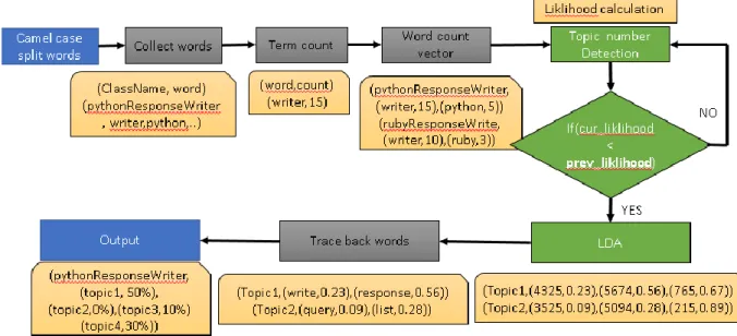
In component identification, the first step is the Latent Dirichlet Allocation (LDA) in which the topics in each class are discovered and the next step is K-Means clustering in which similar classes are clustered. The camel case split details of the class and package forms the input for LDA. Each line in the file represents a document. Each class is represented as a document in LDA. Each word from the document is tokenized. The vocabulary is used to match the words in the document. The stop words are eliminated from the set of words in the document. This eliminates the most frequently occurring words and hence helps in giving more accurate result for topic discovery. The words are then converted to term count vectors and sent to LDA. Then the hyper parameter of LDA is set with the following value: seedValue -> 45. Then LDA is executed to get the topics in each class. This result is converted such that the percentage of each class is determined in each class. The code below gives the optimal way to find the number of topics in LDA.
The likelihood calculation is an iterative process and continues till the current values is greater than the previous. The optimal topic identified for Apache Solr is 31. This value is determined as the likelihood is the highest when topic number is 31 and starts decreasing when it is 32 and so on. Figure 15 illustrates an example of LDA.
42
Figure 15: Example illustrating LDA
Table 5 shows the transition from LDA output to K-Means input. The double value is converted to percentage.
Table 5: Transition from LDA Output to K-Means input
LDA Output K-Means Input
org.apache.solr.handler.component:StatsCo mponent,Map (topic2 -> 39.700244565601274, topic6 -> 19.359571904941955, topic5 -> 12.824371981401619, topic4 -> 6.453504309807704, topic3 -> 15.950295060568461, topic7 -> 5.712012177678984) org.apache.solr.handler.component:StatsCompo nent, (topic1->0, Topic2->39.700244565601274, Topic3->15.950295060568461, Topic4->6.453504309807704, Topic5->12.824371981401619, Topic6->19.359571904941955, Topic7->5.712012177678984) (org.apache.solr.core:MMapDirectoryFactor y,Map (topic2 -> 10.164006817299361, org.apache.solr.core:MMapDirectoryFactory, topic1->16.587662929867523, topic2->10.164006817299361,
43 topic6 -> 39.170171375834485, topic1 -> 16.587662929867523, topic5 -> 18.248055494319253, topic4 -> 3.112555083220393, topic3 -> 8.932104764379242, topic7 -> 3.785443535079752) topic3->8.932104764379242, topic4->3.112555083220393, topic5->18.248055494319253, topic6->39.170171375834485, topic7->3.785443535079752)
The input for K-Means algorithm is again split and a matrix is formed based on the distribution of topics percentage in each class. To compute the best value of number of clusters, Sum of Squared Errors method is used to determine the cluster number K based on the cost to compute K-Means Dynamic cluster number identification makes the model optimal for any given project. It is very important to select the correct parameters for K-Means, especially the
number of clusters. Sum of Squared Errors method is used for identifying the number of clusters in K-Means. The automated approach follows the steps in which the cost of computing K-Means is calculated for each cluster. It is an iterative process to calculate the cost by increasing the cluster number. Once the difference between the costs of consecutive cluster number becomes stagnant, that cluster number is identified. This determines the number of clusters in K-Means algorithm.
44
Finding the number of clusters is an iterative process and hence K-Means cost is calculated to check if the difference between the last 4 values is minimal. For Apache Solr the number of clusters is 169 as the line in the graph starts becoming almost like a straight line.
Hence, the number of clusters is dynamically found for K-Means clustering. Figure 16 gives an example of K-Means algorithm. Most of the handlers are grouped in Cluster 1 TermsComponent, XMLLoader, LeaderElector, TransactionLog are grouped in Component 1 and so on.
Figure 16: Example illustrating K-Means
org.apach.e.solr.handler.component:TermsComponent,26.0457,0,20.9,74,52.97 org.apache.solr.rest:RestManager,16.407,19.680256,20.511987277161197,5.18385,12.3732786,21.259472,4.0275 org.apache.solr.rest.schema:SolrQueryParserDefaultOperatorResource,11.7463,14.98,22.884,1.949,27.75,10.352,10.86186 org.apache.solr.handler.loader:XMLLoader,6.549,17.72411,7.475702,12. 759,14.472734229783788,32.6904816,8.351964 org.apache.solr.cloud:LeaderElector,18.59636840195819,7.539142,31.2993,8.085,15.84304,15.8654,2.807972456377 org.apache.solr.cloud:ShardLeaderElectionContext,6.2161,11.315,30.984812,8.70451795780556,7.55,27.9617648,7.196 org.apache.solr.search:QueryResultKey,19.993159427148825,7.8,2.95793815,7.32697835,45.1374757,8.3021729,8.2956 Cluster 0 RestManager JsonUpdateRequestHandler SolrQueryResponse Cluster 1 TermsComponent XMLLoader LeaderElector TransactionLog Cluster n QueryResultKey SharedLeaderElector DumpRequestHandler
45
5.4 Feature Discovery
The names of all the code entities identified during the features extraction stage are then passed through a keywords analyzer function. The keywords analysis stage has been split into 2 stages.
1) The important words in the document, which means the cluster related words in this case, are identified using the TF-IDF algorithm. A two way processing is done. One with only the class and package related details. The other is more details about the class like methods, attributes, class and package.
2) The results of both the algorithm are combined together to get more appropriate and accurate results.
These most frequently used words help determine the semantics of the project. Instead of using a simple frequency count of words we have used TF-IDF which stands for Term Frequency–Inverse Document Frequency is a numerical statistics technique which is used to analyze the importance of a word within a document in a given collection. The TF-IDF value proportionally increases to the number of times a word is present in the document, but is offset by the word frequency in the corpus. This helps in the adjustment of the fact that generally few words might appear more frequently. Figure 17 illustrates TF-IDF.
46
Figure 17: Example illustrating TF-IDF
This probabilistic model helps in identifying the important words not only based on frequency, but also based on the comparison of the word with the entire document and project. In this case each document is the list of class details in each cluster and the output are the words which is the functionality in each cluster.
47 CHAPTER 6
RESULTS AND EVALUATION 6.1 Overview
This chapter presents the results and evaluation of the thesis research. Section 6.2 explains about the accuracy measure of the results. Section 6.3 has the proof of selecting a certain value for making the algorithm dynamic with the help of graphs. The verification of the existing approach is explained in section 6.4. The results of the research are shown in section 6.5.
6.2 Accuracy
Using a case-study illustrating the automatic discovery of components and features of Apache Solr, we demonstrated the accuracy and scalability of our proposed model compared with manual evaluation by software architecture experts as a baseline. Another case study on Hadoop is also performed to understand the functionality of the automated tool for feature generation.
Apache Solr [10] is an open source project that aims to support highly scalable, fault tolerant and reliable, providing automated failover and recovery , centralized configuration, distributed indexing, load-balanced querying and replication, and many more. Solr, which is written in Java, is an enterprise open source platform for search from the Apache Lucene project. It is a highly scalable and fault-tolerance system and hence it is used one of the popular search engine. Solr has various features such as complete-text search, real-time indexing, hit highlighting, dynamic clustering, rich document and NoSQL feature handling, faceted search, database integration.
48
The proposed approach includes component identification and feature recovery. The first stage in the process is conversion of Solr project to RDF format from Java. Below are the statistics of Solr project generated using the RDFCoder library. Solr is one of the big and famous open source projects which contains almost 737 classes. It is a good use case for automatic feature-based analysis. The main assumption as mentioned is that the names of the elements or entities in the code base are meaningful and follow the standard naming convention in camel case. Table 6 is the Solr Statistics.
Table 6: Solr Statistics Generated by RDFCoder
The following figure 18 gives a pie chart representation of the Solr statistics.
Figure 18: Apache Solr statistics
Parsed Files 737 Parsed Classes 737 Parsed Attributes 3739 Parsed Methods 6698 737 6678 3739
49
The final results from the analysis prove that the approach gives accurate results when compared with the manual analysis of the Apache Solr project. Three different approaches are used in this process and hence comparison of accuracy for all three approaches are visualized in a graph.
Approach 1:
In this approach, TF-IDF is executed with only class and package details. The importance is given only to class and package level details. Hence, all the features might not be discovered as the code level details are not captured.
Approach 2:
In this approach, TF-IDF is executed with class, method, attribute details and hence inner details of the code are captured. Since many details are captured, this approach results in a lot of features for a project. A high number of features that were generated from this approach, might not be interesting for feature discovery.
Hybrid Approach:
The common features from Approach 1 and Approach 2 will be considered. This approach is better because more importance is given to the words in class and package level, than the method and attribute level. The hybrid approach combining the features gives more accurate results than the separate approaches.
The following graph shows the number of features in all three approaches. It is evident that the number of features in the hybrid approach is moderate and shows a good match with the features from the manual analysis. The feature variants are the features with their full names, as used in the projects. The features variants for the combined feature set are the union of feature variants set from approach 1 and approach 2. Figure 19 shows the number of feature and feature
50
variants in 3 different categories and the final feature and feature variants are generated by the hybrid approach. Newly discovered features are given in section 6.5.
Figure 19: Number of feature and feature variants in Apache Solr
Jaccard index is used in the verification process. The Jaccard [22] index, also popularly known as the Jaccard similarity coefficient, is a one of the statistics which is used for comparing the diversity and similarity of the given set of sample. It finds similarity between finite sets of sample, and is defined by the expression below:
(We define J(A,B) = 1, if A and B are both empty.)
The Jaccard distance is found by the complimentary of the Jaccard coefficient. To find the complimentary, the Jaccard coefficient has to be subtracted from 1. This formula will be