Data Warehousing & OLAP

(1)

Data Warehousing & OLAP

 

Data Mining:

 

Concepts and Techniques

 

— Chapter 3 —

Jiawei Han

and

An Introduction to Database Systems

C.J.Date,

(2)

 

What is Data Warehousing?

 

What is OLAP?

 

What is a Data Cube, what is a Cuboid?

 

What is ROLAP, MOLAP, HOLAP

What is Data Warehouse?

 

Defined in many different ways, but not

rigorously

•  A decision support database that is maintained separately

from the organization’s operational database

•  Support information processing by providing a solid platform of consolidated, historical data for analysis.

 

“A data warehouse is a subject-oriented, integrated,

time-variant, and nonvolatile collection of data in

support of management’s decision-making process.”—

W. H. Inmon

 

Data warehousing:

(3)

Data Warehouse—

 

Subject-Oriented

 

Organized around major subjects, such as

customer,

product, sales

 

Focusing on the modeling and analysis of data for

decision makers,

not on daily

operations or

transaction processing

 

Provide

a simple and concise

view around particular

subject issues by

excluding data that are not useful in

the decision support process

Data Warehouse—

 

Integrated

 

Constructed by integrating

multiple

,

heterogeneous

data sources

  relational databases, flat files, on-line transaction records

 

Data cleaning and data integration techniques are

applied.

  Ensure consistency in naming conventions, encoding structures, attribute measures, etc. among different data sources

•  E.g., Hotel price: currency, tax, breakfast covered, etc.   When data is moved to the warehouse, it is converted.

(4)

Data Warehouse—

 

Time Variant

 

The time horizon for the data warehouse is significantly

longer than that of operational systems

  Operational database: current value data

  Data warehouse data: provide information from a historical

perspective (e.g., past 5-10 years)

 

Every key structure in the data warehouse

  Contains an element of time, explicitly or implicitly

  But the key of operational data may or may not contain “time element”

Data Warehouse—

 

Nonvolatile

 

A

physically separate store

of data transformed

from the operational environment

 

Operational

update of data does not occur

in the

data warehouse environment

 

Does not require transaction processing, recovery,

and concurrency control mechanisms

(5)

Data Warehouse vs.

Heterogeneous DBMS

  Traditional heterogeneous DB integration: A query driven approach

  Build wrappers/mediators on top of heterogeneous databases

  When a query is posed to a client site, a meta-dictionary is used to translate the query into queries appropriate for individual heterogeneous sites involved, and the results are integrated into a global answer set

  Complex information filtering, compete for resources

  Data warehouse: update-driven, high performance

  Information from heterogeneous sources is integrated in advance and stored in warehouses for direct query and analysis

OLTP vs. OLAP

OLTP OLAP

users clerk, IT professional knowledge worker

function day to day operations decision support

DB design application-oriented subject-oriented

data current, up-to-date detailed, flat relational isolated

historical,

summarized, multidimensional integrated, consolidated

usage repetitive ad-hoc

access read/write

index/hash on prim. key lots of scans

unit of work short, simple transaction complex query

# records accessed tens millions

#users thousands hundreds

DB size 100MB-GB 100GB-TB

(6)

Why Separate Data

Warehouse?

  High performance for both systems

  DBMS— tuned for OLTP: access methods, indexing, concurrency control, recovery

  Warehouse—tuned for OLAP: complex OLAP queries, multidimensional view, consolidation

  Different functions and different data:

  _{missing data}_{: Decision support requires historical data which operational}

DBs do not typically maintain

  _{data consolidation}_{: DS requires consolidation (}_aggregation, summarization) of data from heterogeneous sources

  _{data quality}_{: different sources typically use}_inconsistent_data

representations, codes and formats which have to be reconciled

  Note: There are more and more systems which perform OLAP

analysis directly on relational databases

What is OLAP?

 

The term OLAP („online analytical

processing“) was coined in a white paper

written for Arbor Software Corp. in

1993

 

Interactive

process of creating, managing,

analyzing and reporting on data

 

Analyzing large quantities of data in

real-time

(7)

OLAP

 

Data is perceived and manipulated as

though it were stored in a

„multi-dimensional array“

 

Ideas are explained in terms of

conventional SQL-styled tables

Data aggregation

 

Data aggregation

(agregação)

in many

different ways

 

The number of possible groupings quickly

becomes large

 

The user has to consider all groupings

 

Analytical processing problem

(8)

 

For two dimensions

 

Spreadsheet (

Excel) with spreadsheet

formulas calculations

 

For more than two dimensions

 

We will require several spreadsheet tables

 

-> Data explosion

Queries for

 

supplier-and-parts database

1)

 

Get the total shipment quantity

2)

 

Get total shipment quantities by supplier

3)

 

Get total shipment quantities by part

(9)

  SP S# P# QTY S1 P1 300 S1 P2 200 S2 P1 300 S2 P2 400 S3 P2 200 S4 P2 200

1. SELECT SUM(QTY) AS TOTQTY

FROM SP

GROUP BY () ;

TOTQTY

(10)

2. SELECT S#, SUM(QTY) AS TOTQTY FROM SP GROUP BY (S#) ; S# TOTQTY S1 500 S2 700 S3 200 S4 200 3. SELECT P#, SUM(QTY) AS TOTQTY FROM SP GROUP BY (P#) ; P# TOTQTY P1 600 P2 1000

(11)

4. SELECT S#, P#, SUM(QTY) AS TOTQTY FROM SP GROUP BY (S#,P#) , S# P# TOTQTY S1 P1 300 S1 P2 200 S2 P1 300 S2 P2 400 S3 P2 200 S4 P2 200

Drawbacks

 

Formulation so many similar but distinct

queries is tedious

 

Executing the queries is expensive

 

Make life easier,

 

more efficient computation

 

Single query

 

GROUPING SETS, ROLLUP, CUBE options

(12)

GROUPING SETS

 

Execute several queries simultaneously

SELECT S#, P#, SUM (QTY) AS TOTQTY

FROM SP

GROUP BY GROUPING SETS ( (S#), (P#) ) ;

Single results table

Not a relation !!

null  missing information

S# P# TOTQTY S1 null 500 S2 null 700 S3 null 200 S4 null 200 null P1 600 null P2 1000

SELECT CASE GROUPING ( S# )

WHEN 1 THEN ‘??‘ ELSE S# AS S#, CASE GROUPING ( P# ) WHEN 1 THEN ‘!!‘ ELSE P# AS P#,

SUM ( QTY ) AS TOTQTY

FROM SP

GROUP BY GROUPING SETS ( ( S# ), ( P# ) );

S# P# TOTQTY S1 !! 500 S2 !! 700 S3 !! 200 S4 !! 200 ?? P1 600 ?? P2 1000

(13)

ROLLUP

SELECT S#,P#, SUM ( QTY ) AS TOTQTY

FROM SP

GROUP BY ROLLUP (S#, P#) ;

GROUP BY GROUPING SETS ( ( S#, P# ), ( S# ) , ( ) )

S# P# TOTQTY S1 P1 300 S1 P2 200 S2 P1 300 S2 P2 400 S3 P2 200 S4 P2 200 S1 null 500 S2 null 700 S3 null 200 S4 null 200 null null 1600

ROLLUP

 

The quantities have been „roll up“

(estender)

for each supplier

 

Rolled up „along supplier dimension“

GROUP BY ROLLUP (A,B,...,Z)

(A,B,...,Z) (A,B,...) (A,B) (A) ()

(14)

CUBE

SELECT S#, P#, SUM ( QTY ) AS TOTQTY

FROM SP

GROUP BY CUBE ( S#, P#) ;

GROUP BY GROUPING SETS ( (S#, P#), ( S# ), ( P# ), ( ) )

S# P# TOTQTY S1 P1 300 S1 P2 200 S2 P1 300 S2 P2 400 S3 P2 200 S4 P2 200 S1 null 500 S2 null 700 S3 null 200 S4 null 200 null P1 600 null P1 1000 null null 1600

CUBE

 

Confusing term CUBE (?)

 

Derived from the fact that in multidimensional

terminology,data values are stored in cells of a

multidimensional array or a hypercube

•  The actual physical storage my differ

 

In our example

•  cube has just two dimensions (supplier, part)

•  The two dimensions are unequal (no square rectangle..)

 

Means „group“ by all possible subsets of the set

(15)

CUBE

 

Means „group“ by all possible subsets of the set

{A, B, ..., Z }

 

M={A, B, ..., Z },

|M|=N

 

Power Set (Algebra)

 

P(M):={U | U

⊆

M},

|P(M)|=2

N

..proof by induction

 

Subset represent different grade of

summarization

 

Data Mining: such a subset is called a

Cuboid

Cross Tabulations

 

Display query results as cross tabulations

 

Formatted as a simple array

 

Example: two dimensions (supplier and

parts)

P1 P2 Total S1 300 200 500 S2 300 400 700 S3 0 200 200 S4 0 200 200 600 1000 1600

(16)

What is a Data Cube?

 

Data Mining definition

 

A data cube, such as sales, allows data to be

modeled and viewed in multiple dimensions

 

Dimension tables, such as

•  item(item_name, brand, type)

•  time(day, week, month, quarter, year) ...hierarchy

 

Fact table contains

measures

(numerical values, such

as dollars_sold) and

keys

to each of the related

dimension tables

Cuboid (Data Mining Definition)

 

Names in data warehousing literature:

 

The n-D cuboid, which holds the lowest level of

summarization, is called a

base cuboid

.. {{A},{B},..}

 

The top most 0-D cuboid, which holds the highest-level

of summarization, is called the

apex cuboid

..{∅}

(17)

Cube: A Lattice of

Cuboids

....(

Power Set)

time,item

time,item,location

time, item, location, supplier

all

time item location supplier

time,location time,supplier item,location item,supplier location,supplier time,item,supplier time,location,supplier item,location,supplier 0-D(apex) cuboid 1-D cuboids 2-D cuboids 3-D cuboids 4-D(base) cuboid

2

4

₌₁₆

Conceptual Modeling of Data

Warehouses

 

Modeling data warehouses: dimensions & measures

instead of relational model

 

Subject, facilitates on-line data analysis oriented

 

Most popular model is the multidimensional model

 

Most common modeling paradigm:

  Star schema

  Data warehouse contains a large central table (fact table) •  Contains the data without redundancy

(18)

Example of Star Schema

time_key day day_of_the_week month quarter year time location_key street city state_or_province country location Sales Fact Table

time_key item_key branch_key location_key units_sold dollars_sold avg_sales Measures item_key item_name brand type supplier_type

item

branch_key branch_name branch_type

branch

Snowflake schema

 

Snowflake schema: A refinement of star

schema where some dimensional hierarchy

is

normalized

into a set of smaller

dimension

tables, forming a shape similar to snowflake

(19)

Schema

time_key day day_of_the_week month quarter year time location_key street city_key location Sales Fact Table

time_key item_key branch_key location_key units_sold dollars_sold avg_sales Measures item_key item_name brand type supplier_key

item

branch_key branch_name branch_type

branch

supplier_key supplier_type

supplier

city_key city state_or_province country city

Fact constellations

 

Fact constellations:

Multiple

fact tables share

dimension tables, viewed as a collection of

stars, therefore called galaxy schema or fact

constellation

(20)

Example of Fact

Constellation

time_key day day_of_the_week month quarter year time location_key street city province_or_state country location Sales Fact Table

time_key item_key branch_key location_key units_sold dollars_sold avg_sales Measures item_key item_name brand type supplier_type item branch_key branch_name branch_type branch

Shipping Fact Table time_key item_key shipper_key from_location to_location dollars_cost units_shipped shipper_key shipper_name location_key shipper_type shipper

Hierarchies

 

Independent variables are often related in

hierarchies (taxonomy)

 

Determine ways in which dependent data can be

aggregated

 

Temporal hierarchy

 

Seconds, minutes, hours, days, weeks, months,

years

 

Same data can be aggregated in many different

ways

 

Same independent variable can belong to different

(21)

Hierarchy - Location

all

Europe

North_America

Mexico

Canada

Spain

Germany

Vancouver

M. Wind

L. Chan

...

all

region

office

country

Toronto

Frankfurt

city

View of Warehouses and

Hierarchies

Specification of hierarchies

 

Schema hierarchy

day < {month < quarter; week} < year

 

Set_grouping hierarchy

(22)

Multidimensional Data

 

Sales volume as a function of product,

month, and region

Product

Month

Dimensions: Product, Location, Time Hierarchical summarization paths

Industry Region Year

Category Country Quarter

Product City Month Week

Office Day

Measures of Data Cube:

 

Three Categories

 

(Depending on the aggregate functions)

 

Distributive

: if the result derived by applying the function to

n

aggregate values

is the same as that derived by

applying the function on

all the data

without partitioning

•  E.g., count(), sum(), min(), max()

 

Algebraic

:

if it can be computed by an algebraic function

with M arguments (where M is a bounded integer), each of

which is obtained by applying a distributive aggregate

function

•  E.g., avg(), min_N(), standard_deviation()

(23)

Drill up and down

 

Drill up:

 

going from a lower level of aggregation to a higher

 

Drill down:

 

means the opposite

 

Difference between drill up and roll up

•  Roll up: creating the desired groupings or aggregations

•  Drill up: accessing the aggregations

 

Example for drill down:

•  Given the total shipment quantity, get the total quantities for each individual supplier

A Sample Data Cube

Total annual sales of TV in Portugal

Date

Pr

oduct

Country

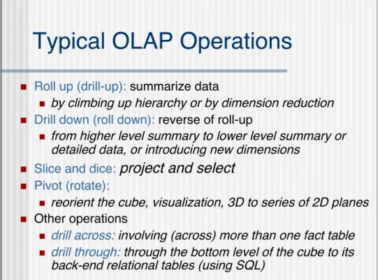
sum sum TV VCRPC 1Qtr 2Qtr 3Qtr 4Qtr Portugal Spain Germany sum

(24)

Typical OLAP Operations

 

Roll up (drill-up):

summarize data

 

by climbing up hierarchy or by dimension reduction

 

Drill down (roll down):

reverse of roll-up

 

from higher level summary to lower level summary or

detailed data, or introducing new dimensions

 

Slice and dice:

project and select

 

Pivot (rotate):

 

reorient the cube, visualization, 3D to series of 2D planes

 

Other operations

 

drill across: involving (across) more than one fact table

 

drill through: through the bottom level of the cube to its

back-end relational tables (using SQL)

Fig. 3.10 Typical OLAP Operations

(25)

Multi-dimensional query

Language

 

No standard yet..

 

DMQL,

MDX

,..

•  MDX was introduced by Microsoft with Microsoft SQL Server OLAP Services in around 1998, as the language component of the OLE DB for OLAP API. More recently, MDX has appeared as part of the XML for Analysis API. Microsoft proposed that the MDX is a standard, and its adoption among application writers and other OLAP providers is steadily increasing.

 

No normalization theory that could serve as a

scientific basis for designing

multi-dimensional

databases

What Is MDX?

 

MDX is Multi Dimensional EXpressions

 

MDX is the syntax for querying an Analysis

Services database

 

MDX is part of the OLE DB for

 

OLAP spec

 

MDX is the key for all advanced analytical

capabilities of

 

(26)

Comparison To SQL

SQL Construct

OLAP construct

SELECT…

(MDX)

CREATE…

DSO object model

DROP…

INSERT…

DELETE…

MDX Basics

 

MDX allows easy navigation in the multi

dimensional space

 

It “understands” the MD concepts of cube,

dimension, level, member

 

and cell

 

It is used for

 

Queries – full statements (SELECT…FROM)

 

Business modeling – defining

 

calculated members using MDX Expressions –

not a full statement

(27)

MDX Queries vs. MDX Expressions

 

MDX Queries

 

Full statements (SELECT…FROM)

 

Usually generated by a query tools and

applications such as Excel

 

MDX Sample App deals in queries

 

MDX Expressions

 

Partial MDX statements

 

Define a calculated member, or a set, or

member properties, etc.

 

Returns a single value (which may

 

be a set)

MDX Constructs

 

Members: an item in a hierarchy

  [John Doe]

  [2001]

  [2001].[Q1].[Jan]

 

Tuple: an intersection of 2 or more members

  ([Product].[Drink].[Beverages], [Customers].[USA])

  ([Product].[Non-Consumable], [2001])

 

Sets: a group of tuples or members

  {[John Doe], [Jane Doe]}

  { ( [Non-Consumable], USA ), ( Beverages, Mexico ) }

  [2001].Children

(28)

Background

Select

on axis (x),

on axis (y),

on axis (z)

From [cubeName]

(29)

Every Cell Has A Name...

(30)

Every Cell Has A Name...

Basic MDX Query

[WITH

MEMBER

SET]

SELECT [<axis_specification> [,

<axis_specification>...]]

FROM [<cube_specification>]

[WHERE [<slicer_specification>]]

(31)

 

A query has one or more dimensions. The query above

has two. (The first three dimensions (=axes) that are

found in MDX queries are known as

rows

,

columns

and

pages

)

SELECT{[Time].[1997].[Q1],[Time].[1997].[Q2]}ON COLUMNS,{[Warehouse].[All Warehouses].[USA]} ON

ROWSFROM WarehouseWHERE ([Measures].[Warehouse Sales])

 

Curled brackets "{}" are used in MDX to represent a set

of members of a dimension or group of dimensions

Sections of a Basic MDX Query

 

Cube

– source cube for query

 

Axes

  Collection of members from different dimensions organized as a set of tuples

  For example, an axis that includes Time and Product

dimensions will result in aggregation along these dimensions (cell will include members of these two dimensions)

 

Members

– selected dimension attributes that are included in output cube

  Measures (facts) of a fact table are treated as members of a Measures dimension

(32)

Example MDX Query

SELECT

{[Measures].[StoreSales]} on columns,

{[Time].[2002].[Q3], [Time].[2002].[Q4]} on rows

FROM SalesCube

(33)

MDX Notation for schema

 

Periods separate schema parts

 

Ex. [Products].[Food].[Dairy]

 

No spaces in names unless square

brackets are used

 

Examples

• Dimension: [Time]

• Hierarchy: [Time].[Fiscal]

• Level: [Time].[Fiscal].[2000].[Q3]

• Member: Time.Fiscal.2000.Q2.May

WITH Operator

 

Use to:

 

Specify a calculated member

 

Define named sets

 

Example

WITH

MEMBER [Measures].[DaysWorked] AS ‘[Measures].[EndDate] – [Measures].[StartDate]’

SELECT

{ [Measures].[StartDate], [Measures].[EndDate], [Measures]. [DaysWorked] } ON COLUMNS,

{ [Employee].[Department] } ON ROWS

(34)

WHERE (slice)

IMPORTANT NOTE:

If a dimension does not appear on a filter axis, the

default member of that dimension is used

 

Usually, the default is the “ALL” member

Common Operators and Functions

 

Comma – construct a set by enumerating tuples

  Ex. {[Time].[2001].[Jan], [Time].[2001].[Feb]. …}

 

Colon – construct a set by specifying a range

  Ex. { [Time].[2001].[Jan] : [Time].[2001].[Nov] }

 

.Members – returns set of all members

  Ex. [Customers].Members

 

Comments

  /* */ - can be multi-line

  // - to end of line

(35)

 

CrossJoin() –

cross-product of members or tuples in two

different sets

  Product all possible combinations

  Ex. Construct a set

  Ex. CrossJoin (

{ [Time].[2000].[Jan] : [Time].[2000].[Dec] },

{ [Product].[Brand].Members } )

. . .

Common Operators and

Functions

(cont’d)

Common Operators and

Functions

(cont’d)

 

Filter() –

reduce a set by including only those elements

that satisfy some criteria

  Arguments •  Boolean Expression •  Set   _{Returns subset}   Ex. Filter ( { [Product].[Brand].Members }, [Measures].[Sales] >= 500 )

(36)

Common Operators and

Functions

(cont’d)

 

Order() –

order a set

  Arguments

•  Ordering criterion

•  Set

•  Flag option (ex. Ascending, descending)

  Hierarchical order can be complex

  Ex. Order ( { [Product].[Brand].Members }, ([Measures].[Sales], [Time].[2000]), BDESC )