ScholarWorks @ UTRGV
ScholarWorks @ UTRGV
Mathematical and Statistical Sciences Faculty
Publications and Presentations
College of Sciences
2020
Effect of Hydraulic Resistivity on a Weakly Nonlinear Thermal
Effect of Hydraulic Resistivity on a Weakly Nonlinear Thermal
Flow in a Porous Layer
Flow in a Porous Layer
Dambaru Bhatta
The University of Texas Rio Grande Valley
Daniel N. Riahi
The University of Texas Rio Grande Valley
Follow this and additional works at:
https://scholarworks.utrgv.edu/mss_fac
Part of the
Mathematics Commons
Recommended Citation
Recommended Citation
Bhatta, Dambaru, and Daniel N. Riahi. 2020. “Effect of Hydraulic Resistivity on a Weakly Nonlinear
Thermal Flow in a Porous Layer.” Journal of Applied Fluid Mechanics 13 (3): 945–55. https://doi.org/
10.29252/jafm.13.03.30207.
This Article is brought to you for free and open access by the College of Sciences at ScholarWorks @ UTRGV. It has been accepted for inclusion in Mathematical and Statistical Sciences Faculty Publications and Presentations by an authorized administrator of ScholarWorks @ UTRGV. For more information, please contact [email protected], [email protected].
J
ournal of
A
pplied
F
luid
M
echanics
, Vol. 13, No. 3, pp. 945-955, 2020.
Available online at
www.jafmonline.net
, ISSN 1735-3572, EISSN 1735-3645.
DOI: 10.29252/jafm.13.03.30207
Effect of Hydraulic Resistivity on a Weakly Nonlinear
Thermal Flow in a Porous Layer
D. Bhatta
1†and D. N. Riahi
21The University of Texas Rio Grande Valley, Edinburg, TX, USA, 78539 2 The University of Texas Rio Grande Valley, Brownsville, TX, USA, 78520
†Corresponding Author Email: [email protected] (Received February 27, 2019; accepted July 24, 2019)
ABSTRACT
Heat and mass transfer through porous media has been a topic of research interest because of its importance in various applications. The flow system in porous media is modelled by a set of partial differential equations. The momentum equation which is derived from Darcy’s law contains a resistivity parameter. We investigate the effect of hydraulic resistivity on a weakly nonlinear thermal flow in a horizontal porous layer. The present study is a realistic study of nonlinear convection flow with variable resistivity whose rate of variation is arbitrary in general. This is a first step for considering more general problems in applications that involve variable resistivity that may include both variations in permeability and viscosity of the porous layer. Such problems are important for understanding properties of underground flow, migration of moisture in fibrous insulations, underground disposal of nuclear waste, welding process, petrochemical generation, drug delivery in vascular tumor, etc. Using weakly non-linear procedure, the linear and first-order systems are derived. The critical Rayleigh number and the critical wave number are obtained from the linear system using the normal mode approach for the two-dimensional case. The linear and first-order systems are solved numerically using the fourth-order Runge-Kutta and shooting methods. Numerical results for the temperature are presented in tabular and graphical forms for different resistivities. Through this study, it is observed that a stabilizing effect on the dependent variables occurs in the case of a positive vertical rate of change in resistivity, whereas a destabilizing effect is noticed in the case of a negative vertical rate of change in resistivity. The results obtained indicate that the convective flow due to the buoyancy force is more effective for weaker resistivity
.
Keywords: Hydraulic resistivity; Weakly nonlinear; Hydro-thermal; Convective flow; Rayleigh number.
NOMENCLATURE
P
perturbed pressure p pressure pb basic state pressureε perturbation parameter i complex unit
k unit vector in the vertical positive z-direction
Rayleigh number critical Rayleigh number T temperature
Θ perturbed temperature
θb basic state temperature
t time variable
(x,y,z) cartesian coordinates perturbed velocity vector U X component of the velocity vector V y component of the velocity vector W z component of the velocity vector
velocity vector basic state velocity vector wavenumber γ resistivity γ0 rate of change in resistivity
2 3D Laplacian
∆ 2D Laplacian
1.
I
NTRODUCTIONFluid flow and heat transfer through a porous medium have been a topic of research interest for last
several decades. A porous medium is a material that consists of a solid material with inter-connected voids or pores. It is characterized by its porosity and the permeability of the medium is the. Darcy’s law
for porous media is taken into account in the momentum equation, which is similar to the Navier-Stokes equation. In natural porous media the distribution of pores with respect to shape and size is not regular. But in typical experiments the quantities of interest are measured over areas that cross many pores and changes of such space averaged quantities may be considered in a regular way and hence are acceptable to theoretical
treatment. Heat transfer through a porous medium is a very common phenomenon. The normal tendency of a fluid to expand due to heating causes a density inversion to occur, if the heating is strong enough, a circulatory motion follows, termed convection. Convection in fluid media is well-studied phenomenon and occurs in many natural settings and in many industrial applications. Mathematical treatment and research on convection in porous media have been presented by many authors through many research articles (Nield and Bejan 2017, Vafai 2005).
Many studies have been presented by various authors to investigate convection in porous media with varying porosity or permeability. Rubin (1981) investigated the onset of thermohaline convection in a porous medium with varying hydraulic resistivity. Vafai (1984) investigated wall effects due to variable porosity. Variable porosity and thermal dispersion effects due to natural convection in an inclined porous cavity were studied by Hsiao (1998). Modal package convection for a porous medium with boundary imperfections was analyzed by Riahi (1996). The effect of variable permeability in porous media was analyzed analytically and numerically by Rees and Pop (2000). Hassanien and Omer (2005) studied the effect of variable permeability in a porous medium. Oliveski and Macrczak (2008) analyzed the effect of variable porosity and Darcy number in a porous cavity. A medium with variable permeability was analyzed by Aldoss (2009). Linear and nonlinear stability for a rotating porous fluid layer was analyzed by Falsaperla et al. (2010). Investigations of Darcy’s law for the flow with Pressure-dependent viscosity in a porous medium were carried out several researched including Nakshatrala and Rajagopal (2011), Fusi, Farina and Rosso (2015). The onset of Bernard-Marangoni convection in composite layers with anisotropic porous material was studied by Gangadharaiah (2016).
Riahi (1989) carried out nonlinear stability analysis in a porous layer with permeable boundaries. The case of a continuous finite bandwidth of convection modes in a horizontal layer was analyzed by Riahi (1996). Convective flows, in a horizontal dendritic porous layer (also known as mushy layer) during alloy solidification, are known to produce undesirable effects in the final form of the alloy. Study on oscillatory modes of nonlinear compositional convection in mushy layers was carried out by Riahi (2009).Muddamallappa et al. (2009) used a modified mushy layer model based on the standard near eutectic approximation. They used linear stability analysis and calculated critical
Rayleigh number for the cases of both constant and variable permeability. However, the issues of nonlinear effects and transition effects on the chimney formation did not feature in their investigation. Bhatta et al. (2010) studied weakly nonlinear convective flow in an active (variable permeability) mushy layer with permeable mush-liquid interface. Bhatta et al. (2012) studied weakly nonlinear convective flows in mushy layers with and without the magnetic effect and permeable mush-liquid interface.
A model for an aquifer which can be treated as porous media was presented by Fowler (1997). Rubin (1982) used Galerkin method to analyze the effects of hydraulic resistivity and thermal diffusivity on stability in a nonhomogeneous aquifer. Bhatta and Riahi (2017) investigated weakly nonlinear hydro-thermal two-dimensional convective flow in a horizontal aquifer by treating it as porous medium. Their investigation was limited to small linear vertical variations in the permeability and thermal conductivity. Wang et al
(2017) presented proper orthogonal decomposition (POD) reduced-order model to solve heat transfer problem for heat exchanger. Recently, Dejam (2018, 2019a, 2019b, 2019c), and Kou and Dejam (2019) presented a series of research work in porous media.
There have been some research studies on the effect of hydraulic resistivity (Rubin 1981; Bhatta and Riahi 2017) as well as related ones on variable permeability with or without magnetic field (Bhatta
et al. 2010, 2012). Bhatta et al. (2010, 2012) studied
nonlinear convective flow in a mushy layer, which is a porous layer formed between the solid and liquid layers during the solidification process of binary alloy. The mushy layer that they considered has variable permeability and hence variable resistivity, and they determine the flow evolution for both cases in the absence or presence of a vertically oriented magnetic field. Bhatta and Riahi (2017) studied convective flow in an aquifer layer with variable resistivity, by under the condition that the rate of change of the resisvity was sufficiently small. Tait et al. (1992) carried out experimental investigation of convective flow in a mushy layer and determined the preferred planform of three-dimensional compositional convection in a mushy layer with variable permeability.
Under severe restriction of small variation, previous theretical studies determined convective flow velocity and temperature for different parameter values. In this paper, we use weakly nonlinear procedure to investigate the effect of the vertical rateof change of resistivity on the solutions for a hydro-thermal convective flow in a horizontal porous medium. The present study is to understand the effects of resistivity variations on the non-linear convective flow, which is a first step for more general problems involving resistivity variations. Such problems are important for understanding properties of underground flow, migration of moisture in fibrous insulations, underground disposal of nuclear waste, welding process, petrochemical generation, drug delivery in vascular
tumor etc. We determine important results, in particular, we found that the convective flow is effective if the resistivity is weak and vice versa a strong resistivity leads to weak flow.
We present the mathematical formulation in section 2 where all the important mathematical equations are derived. Section 3 elaborates the solution procedure with the usage of weakly nonlinear method. Normal mode approach for the two dimensional case is derived in section 4. Numerical results and discussion are presented in section 5.
Section 6 summarizes the procedure and conclusions of this study. Some derivations of the main equations presented in section 3 are added in the Appendix.
2.
M
ATHEMATICALF
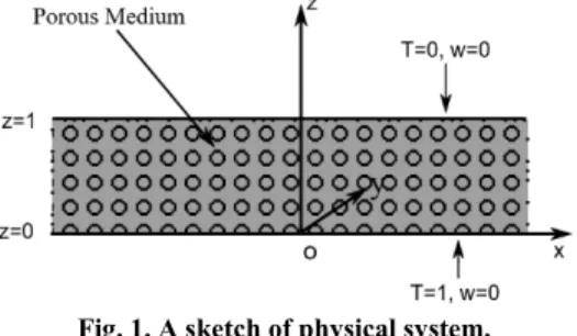
ORMULATIONHere, we consider a horizontal porous medium bounded above and below by impermeable boundaries and heated from below. The horizontal xy-plane is taken as the bottom boundary of the medium, and z-axis is vertical and positive upward. The geometry of the physical system is shown in Fig.1.
Fig. 1. A sketch of physical system.
The governing equation for nondimensional system can be expressed as (Rubin 1982)
. 0 (1) 0 (2) . (3) Here , γ, T , p, , t and , respectively, represent the velocity, resistivity, temperature, pressure, Rayleigh number, time and unit vector in the upward vertical direction. This system consists of the continuity equation, the Darcy equation and the heat equation. For steady state solution, all dependent variables ( , T , p ) are functions of x,y,z. Here, we assume a linear vertical variation in resistivity γ as
1 , (4) where γ0 is a constant which is the vertical rate of
change of the resistivity. The boundary conditions are
1, 0 0 (5) 0, 0 1 (6) where w is the vertical z-component of . A schematic diagram of the convection caused by the
heat difference between the bottom and top layers is shown in Fig.2.
Fig. 2. Convection due to a heated bottom.
3.
S
OLUTIONP
ROCEDUREWe perturb the system given by (1-3) as follows
, , , ,
, , , , , , , , . (7) Here, θb, ,pb are the basic steady state solutions of
system with no flow and Θ, , P are perturbed solutions. The perturbation parameter is given by ε = ( − c)/ 1 > 0 i.e., = c +ε 1, where c is the
critical Rayleigh number and 1 is the nonlinear
contribution to beyond the critical number.
3.1 Basic State System and its Solutions
Using (7) in (1) through (3) and by comparing the coefficients of ε0 as the basic state system with no flow, we have
0, 0, 0 (8) with boundary conditions θb = 1 at z = 0 and θb = 0 =
pb at = 1. Now, by solving the basic state system
(8), we can express the solutions as
1 , 2 1 , 0.
3.2 Perturbed System
Using (7) in the system given by (1-3), we obtain a system in terms of the perturbed variables as follows:
. 0 (9) (10) . . (11) and the boundary conditions become Θ=W = 0 at = 0, 1. Here, W is the vertical z-component of . Now, expressing Θ(x,y,z) and W (x,y,z) as
⋯ (12) ⋯ (13) and the work shown in the Appendix, we obtain different order systems, namely, the linear and the
first-order. Subindex is used to denote various orders.
3.2.1 Linear System
Putting Θ, W given by (12), (13) in the Eqs. (25) and (26) given in the Appendix, the linear system can be expressed by the following equations:
∆ 0 (14) 0, (15) with the boundary conditions Θ0 = W0 = 0 at = 0,
1.
3.2.2 First-Order System
Putting Θ, W given by (12), (13) in the Eqs. (25) and (26), the first-order system can be expressed as:
∆ ∆ (16)
0
.
(17)and the boundary conditions are Θ1 =W1 = 0 at =
0,1.
4.
2-
DS
OLUTIONS: N
ORMALM
ODEA
PPROACHNow, we consider the two dimensional case. Using the normal mode approach, we take the following forms for the linear solutions
, , , , , (18) where α denotes the wave number. As derived in the Appendix, the normal mode linear solutions satisfy
1 0
(19) 0 (20) with boundary conditions = = 0 at = 0, 1. For the normal mode first-order solutions, we have two parts: one is called one-alpha mode due to the presence of eiαxand the other called two-alpha mode
due to the presence of e2iαx. These satisfy (as derived
in the Appendix) 1 (21) 0 (22) with = = 0 = 0 at = 0, 1 and 1 4 4 0 (23) (24) with = = 0 = 0 at = 0, 1.
5.
N
UMERICALR
ESULTSA
NDD
ISCUSSIONIn obtaining the numerical solutions, the fourth-order Runge-Kutta method (RK4) is used in combination with the shooting method (Kincaid and Cheney, 2002). Runge-Kutta methods are numerical procedures used to solve a first-order ordinary differential equation (ODE) with a given initial value, i.e., to solve an IVP (initial value problem). These methods are also used to solve a system of first-order ordinary differential equations with given initial conditions. Higher-order ODE can be solved by expressing the ODE as a system of first-order ODEs. Advantages of Runge-Kutta methods over Taylor’s series methods are that they do not require computation and evaluation of the derivatives which can be very complicated and time consuming. In this work, we use the fourth-order Runge-Kutta method (RK4). It is widely used due to its simplicity in implementation and higher-order accuracy up to the fourth-order. Higher-order Runge-Kutta methods are less attractive than the classical fourth-order due to a higher number of function evaluations. The shooting method is a numerical method used to solve a boundary value problem (BVP) by converting it to an IVP. This method allows one to shoot out trajectories for possible solutions in different directions until a trajectory that has the given boundary values is found. For solving the ODE systems appearing in this work, the codes are written in the Java programming language and for graphing the results, MATLAB is used.
To obtain the critical Rayleigh number and wave numbers, we solve the linear system (19)-(20). We use the fourth order Runge-Kutta method together with the shooing method for a particular value of γ0
by varying the wave number and Rayleigh number and then obtain the minimum Rayleigh number (which is called the critical Rayleigh number), and the corresponding wave number (known as the critical wave number). The critical Rayleigh numbers and the critical wave numbers obtained numerically for different values of γ0 are shown in
Table-1.
It is observed from the Table-1 that higher resistivity resistivity is stabilizing while smaller resistivity is destabilizing. When the rate of change in resistivity, γ0, is zero, it reduces to the standard problem of
constant resistivity where the critical wave number and critical Rayleigh number are known to be π and 4π2, respectively, which match the values computed
in Table-1 (3rd column).
Table 1 Critical wave numbers and Rayleigh numbers
γ
0 -0.5 0.0 0.6 1.4α
c 3.14021 3.14159 3.14095 3.13928 28.95956 39.47842 50.79039 64.83265The marginal stability curves for different values of γ0 are displayed in Fig.3.
Fig. 3. Marginal stability curves for various γ0. The marginal stability curves make it clear that stability region is effected by γ0, the vertical rate of
change in resistivity. For smaller resistivity parameter, unstable region increases. Higher resistivity parameter implies higher stability. Table-2 displays the linar solutions (z) for γ0 =
0.0, 0.6 and -0.5. It is observed from our computational work that the linear solution, (z), has the maximum value of 0.01613 at z = 0.5 for γ0=0, and it is symmetric about the middle of the
layer, z = 0.5. It has a maximum value of 0.02040 at z =0.53 for γ0 = −0.5, and a maximum value of
0.01337 at z=0.48 for γ0 = 0.6.
The linear solutions for the temperature, (z), for different values of γ0 are presented in Fig.4.
Fig. 4. Linear (z) for various γ0. From Fig.4, it is observed that for γ0 = 0.0, the
temperature has a maximum value at the middle of the layer, i.e., at z = 0.5 and temperature is symmetric about the middle of the layer. The maximum value of the temperature shifts downward in the layer for positive values of γ0 and the maximum value of the
temperature moves upward for negative values of γ0.
As fluid is moving upward due to the convection process, the flow amplitude reaches a maximum below the mid-plane if the vertical rate of change of resistivity is positive. This maximum value moves downward with the increasing such magnitude of the
vertical rate of change of resistivity. However,
flow amplitude reaches a maximum above the mid-plane if the vertical rate of change of resistivity is negative, and such maximum value moves further upward with the increasing the magnitude of such negative vertical rate of change.
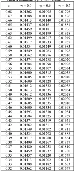
Table 2 Solutions (z) for various γ0 γ0 = 0.0 γ0 = 0.6 γ0 = -0.5 0.68 0.01362 0.01095 0.01796 0.67 0.01388 0.01118 0.01826 0.66 0.01413 0.01140 0.01855 0.65 0.01437 0.01161 0.01881 0.64 0.01459 0.01181 0.01906 0.63 0.01480 0.01199 0.01928 0.62 0.01499 0.01217 0.01949 0.61 0.01517 0.01233 0.01967 0.60 0.01534 0.01249 0.01983 0.59 0.01549 0.01263 0.01998 0.58 0.01562 0.01276 0.02010 0.57 0.01574 0.01288 0.02020 0.56 0.01584 0.01298 0.02028 0.55 0.01593 0.01307 0.02034 0.54 0.01600 0.01315 0.02038 0.53 0.01605 0.01322 0.02040 0.52 0.01609 0.01328 0.02039 0.51 0.01612 0.01332 0.02038 0.50 0.01613 0.01335 0.02034 0.49 0.01612 0.01336 0.02028 0.48 0.01609 0.01337 0.02020 0.47 0.01605 0.01335 0.02010 0.46 0.01600 0.01334 0.01998 0.45 0.01593 0.01330 0.01984 0.44 0.01584 0.01325 0.01969 0.43 0.01574 0.01319 0.01951 0.42 0.01562 0.01311 0.01932 0.41 0.01549 0.01302 0.01911 0.40 0.01534 0.01292 0.01888 0.39 0.01517 0.01280 0.01864 0.38 0.01499 0.01267 0.01837 0.37 0.01480 0.01253 0.01810 0.36 0.01459 0.01237 0.01780 0.35 0.01437 0.01220 0.01749 0.34 0.01413 0.01202 0.01717 0.33 0.01388 0.01182 0.01683 0.32 0.01362 0.01162 0.01647 Figure 5 displays the two dimensional results for the linear solution Θ0(x,z) for γ0 = 0.0 for one period in
x-direction. For γ0 = 0.0, The maximum value occurs
at the center of the domain, i.e., at (0.0, 0.5). The minimums occur in the middle with respect to z, i.e., at z = 0.5, and at both ends of the period with respect x, i.e., at x = −1.0 and x = 1.0. Result is symmetric with respect to x = 0 and z = 0. Similar results are obeserved for the velocity component, W0(x,z).
Computed result for the linear solution of the temperature, Θ0(x,z), for γ0 = 1.4 and γ0 = −1.0 is
shown in Fig.6. The maximum values occur at x = 0 and the minimum values occur at both end of the period with respect to x. But these values shift towards the bottom of the layer for positive γ0 and
towards the top of the layer for negative γ0. Similar
results are obeserved for the velocity component, W0(x,z).
Fig. 5. Linear Solution Θ0(x,z) for γ0 = 0.0.
Fig. 6. Linear solutionΘ0(x,z) for γ0 = 1.4 and γ0=−1.0.
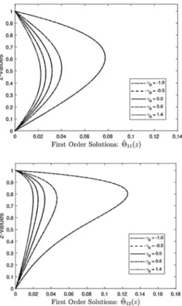
The first-order solutions (one-alpha and two-alpha modes) for the first-order temperatures, Θ (z) and Θ (z), are displayed in Fig.7. In all computations, we use R1 = 1.0. For one-alpha mode, the maximum
values of the dependent variables shift down-ward in the layer for positive values of γ0 and the maximum
values move upward for negative values of γ0. But,
for two-alpha mode, the maximum values of the dependent variables shift upward for any values of γ0. Both solutions have smaller values for positive γ0
than those values for γ0 = 0 and have higher values
for negative γ0 the than the values for γ0 = 0. Two
alpha mode results dominate one alpha mode results for both dependent variables. Similar results hold for the vertical components of the velocity, W (z) and W (z).
Fig. 7. First-order solutions (z) and (z) for various γ0.
Figure 8 displays the two dimensional result for the first-order for the temperature, Θ11(x,z), for γ0 = 0.0
for one period in x-direction. The maximum value for is obtained at (0.0, 0.5). The minimums occur at z = 0.5, and at both ends for x, i.e., at x = −1.0 and x = 1.0. For the one-alpha solution for the velocity component, W11(x,z), similar behavior is observed.
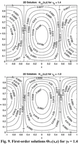
Computed results for the first-order one-alpha solutions for the temperature, Θ11(x,z), for γ0 = 1.4
and γ0 = −1.0 are shown in Fig.9. The maximum
values occur at x = 0 and the minimum values occur at both end of the period of x. But these values shift upward in the layer for negative γ0 and downwards
for positive γ0. Similar results hold for the velocity
component, W11(x,z).
Fig. 9. First-order solutions Θ11(x,z) for γ0 = 1.4
and γ0 = −1.0.
Figure10 shows the solution for the first-order two-alpha mode for the temperature, Θ12(x,z), for γ0 =
0.0. The maximum and minimum values shift up-ward. Result is symmetric about x = 0. Similar result is observed for the velocity component, W12(x,z).
Fig. 10. First-order solution Θ12(x,z) for various γ0 = 0.0.
Table-3 displays the combined first-order temperature Θ (z) = Θ (z) + (z) for various γ0= 0.0, 0.6 and -0.5.
Table 3 Solution (z) for various γ0 γ0 = 0.0 γ0 = 0.6 γ0 = -0.5 0.66 0.05908 0.04667 0.07994 0.65 0.05925 0.04688 0.07997 0.64 0.05938 0.04705 0.07993 0.63 0.05946 0.04720 0.07982 0.62 0.05950 0.04731 0.07965 0.61 0.05949 0.04738 0.07942 0.60 0.05945 0.04743 0.07913 0.59 0.05936 0.04744 0.07878 0.58 0.05923 0.04743 0.07838 0.57 0.05906 0.04738 0.07792 0.56 0.05884 0.04730 0.07741 0.55 0.05860 0.04719 0.07684 0.54 0.05831 0.04706 0.07623 0.53 0.05798 0.04689 0.07557 0.52 0.05761 0.04669 0.07486 0.51 0.05721 0.04646 0.07411 0.50 0.05677 0.04620 0.07331 It is observed from our computational results presented in Table 3 that the first-order solution (Θ (z) = Θ (z) + (z)) has the maximum value of 0.05950 at z = 0.62 for γ0 = 0. It has a maximum
value of 0.07997 at z = 0.65 for γ0 = −0.5, and a
maximum value of 0.04744 at z = 0.59 γ0 = 0.6.
The first-order solutions for the temperature, Θ (z),
for different values of γ0 are presented in Fig.11. The
maximum values shift upward (higher z) in the layer for any values of γ0. Solutions have smaller values
for positive γ0 than those values for γ0 = 0 and have
higher values for negative γ0 than those for γ0 = 0.
For the vertical component of the velocity, W (z), similar results are observed.
Fig. 11. First-order solution (z) for various γ0. Fig.12 displays the two dimensional results for the first-order (combined one-alpha and two-alpha) solution for the temperature, Θ1(x,z), for γ0 = 0.0.
The maximum value occurs at x = 0. The minimum values for Θ1(x,z) not at the end, but inside the period
Fig. 12. First-order solution Θ1(x,z) for γ0 = 0.0. Results for the first-order solutions for temperature, Θ1(x,z), for γ0 = 1.4 and γ0 = −1.0 are presented in
Fig.13. The maximum and minimum values shift upward in the layer for negative γ0. Results are
symmetric with respect to x = 0.
Fig. 13. First-order solutions Θ1(x,z) for γ0 = 1.4
and γ0 = −1.0.
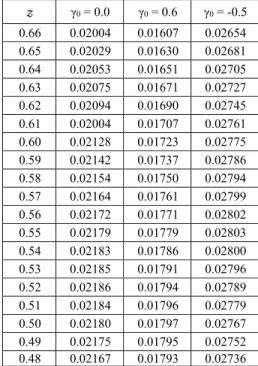
Table-4 displays the nonlinear temperature Θ +εΘ for various γ0 = 0.0, 0.652and -0.5.
Table 4 Solution +ε for various γ0
γ0 = 0.0 γ0 = 0.6 γ0 = -0.5 0.66 0.02004 0.01607 0.02654 0.65 0.02029 0.01630 0.02681 0.64 0.02053 0.01651 0.02705 0.63 0.02075 0.01671 0.02727 0.62 0.02094 0.01690 0.02745 0.61 0.02004 0.01707 0.02761 0.60 0.02128 0.01723 0.02775 0.59 0.02142 0.01737 0.02786 0.58 0.02154 0.01750 0.02794 0.57 0.02164 0.01761 0.02799 0.56 0.02172 0.01771 0.02802 0.55 0.02179 0.01779 0.02803 0.54 0.02183 0.01786 0.02800 0.53 0.02185 0.01791 0.02796 0.52 0.02186 0.01794 0.02789 0.51 0.02184 0.01796 0.02779 0.50 0.02180 0.01797 0.02767 0.49 0.02175 0.01795 0.02752 0.48 0.02167 0.01793 0.02736 It is observed from our computational results presented in Table-4 that the nonlinear solution, Θ +εΘ (z), has the maximum value of 0.02186 at z = 0.52 for γ0 = 0. We use ε = 0.1 It has a
maximum value of 0.02803 at z = 0.55 for γ0 = −0.5,
and a maximum value of for 0.01797 at z = 0.50 γ0 =
0.6.
Results for the nonlinear temperature, Θ +εΘ (z), for different values of γ0 are presented in Fig.14.
Negative γ0 has destabilizing effect and positive γ0
has stabilizing effect on the flow.
Fig. 14. Linear and first-order combined solutions for temperature.
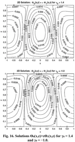
Figure 15 displays the two dimensional results for Θ0(x,z) + εΘ1(x,z) for γ0 = 0.0. The maximum value
occurs at x = 0. The minimum values for Θ1(x,z)
appear inside the period of x, not at the end. Results for Θ0(x,z) + εΘ1(x,z) with γ0 = 1.4 and γ0 =
−1.0 are presented in Fig.16. The maximum and minimum values shift upward in the layer for
negative γ0. All the results are symmetric with respect to x = 0. Similar results are observed for velocity component, W0(x,z) + εW1(x,z) Here are the
highlights of the findings from this work:
• The critical Rayleigh numbers and marginal stability curves indicate that stability region is effected by the resistivity.
• When the vertical rate of change in resistivity, γ0, is
zero, it reduces to the standard problem of constant resistivity where the critical wave number and critical Rayleigh number are known to be π and 4π2, respectively, which match the values
computed in Table 1 (3rd column).
• It is observed that for γ0 = 0.0, the linear solution
Θ0 has a maximum value at the middle of the layer,
and is symmetric about the middle of the layer. The maximum value of Θ0 shifts downward in the layer
for positive values of γ0 and its maximum value
moves upward for negative values of γ0.
• It is observed that the maximun values for the first-order solution, (Θ = Θ + ), shift to the upper half plane for any value of γ0. At x = 0, it is
observed that the first-order solution has the maximum value of 0.05950 at z = 0.62 for γ0 = 0.
It has a maximum value of 0.07997 at z = 0.65 for γ0 = −0.5, and a maximum value of for 0.04744 at
z = 0.59 γ0 = 0.6.
• The contribution of the linear and first-order solutions to temperature at the middle of the layer (z = 0.5) for x = 0, are 0.02186, 0.01797, and 0.02803 for the respective values 0.0, 0.6, and -0.5 of the resistivity parameter. Computational results for the nonlinear solutions demonstrate that buoyancy force and the resulting convective flow quantities are more effective above the mid-plane z = 0.5 if resistivity is weaker. The convective temperature decreases with increasing resistivity, while it increases with decreasing resistivity. • For a positive vertical rate of change in resistivity,
the flow and temperature are stabilizing and their magnitudes are lower in region near the upper boundary, while for a negative vertical rate of change in resistivity, the flow and temperature are destabilizing and their magnitudes are higher in region near the upper boundary.
Fig. 15. Linear and first-order combined solution for γ0 = 0.0.
Fig. 16. Solutions Θ0(x,z)+εΘ1(x,z) for γ0 = 1.4
and γ0 = −1.0.
6.
S
UMMARYA
NDC
ONCLUSIONSHere we study the effect of the vertical rate of change in resistivity on a hydro-thermal convective flow in a porous medium. Based on the critical Rayleigh number and the critical wave number computed from the linear system, we derived the first-order system using weakly non-linear procedure. We used the fourth-order Runge-Kutta method in combination with the shooting method to solve linear and first-order systems numerically. Results indicate a stabilizing effect on the temperature and flow for a positive vertical rate of change in resistivity, whereas a destabilizing effect is noticed for a negative rate of change. It is observed that the convective flow driven by the buoyancy force is more effective if resistivity is weaker, while the opposite result holds for a stronger resistivity effect. Both convective temperature and velocity decrease with increasing resistivity, while they increase with decreasing resistivity.
In addition, flow is asymmetric with respect to the middle of the layer for a non-zero rate of change in resistivity. The maximum values for the temperature and velocity shift downward for a positive vertical rate of change in resistivity and upward for a negative rate of change. Advantage of this study is that it is a first step for future extension to more general variable hydraulic resistivity. The present work also provides understanding the nature of the
nonlinear flow as is affected by presence of variable resistivity whose rate of change is arbitrary. Earlier studies only used small variation. The current study doesn’t have that restriction. Disadvantage of the present study is its limitation for linear variation of resistivity, two-dimensionality of the problem, and the more involved nonlinear second order solutions that are not provided. Future studies may include extending the current work to incorporate nonlinear second-order system and three dimensional extension, and stability of such primary flow solutions.
A
CKNOWLEDGMENTThe authors would like to offer a special thanks to the reviewers for their constructive comments which were very helpful to improve the quality of the paper.
A
PPENDIXElimination of the Pressure
We eliminate the pressure from the Eq. (10) using the poloidal ( ) and toroidal ( ) representations of (since . 0 , Chandrasekhar 1981) which is given by
, , ,
,
Thus, we have W = −∆ φ where ∆ . After elimination of pressure by taking the vertical component of the double curl of the Eq. (10), the perturbed system becomes:
∆ ∆ (25)
ε . (26) Where , .
The boundary conditions are Θ = W = 0 at = 0, 1.
2-D Normal Mode Solutions
Now, we consider the two dimensional case. Using the normal mode approach, we express the linear solutions as
, , , ,
where α denotes the wave number. Thus, we have ,
,
Using the above equations in the linear system (14)-(15), we obtain
1 0
0 (27)
with boundary conditions Θ = 0 = 0 at = 0, 1. For the first-order solutions, we have two parts: one is called one-alpha mode due to the presence of eiαx
and the other called two-alpha mode due to the presence of e2iαx . Thus for the temperature, the
first-order solution Θ1(x, ) = Θ11(x, ) + Θ12(x, ), we write Θ , Θ Θ , Θ which yield , , 4
Also for the velocity component, the first-order W1(x, ) = W11(x, ) + W12(x, ) where W
W and W W , similar
results hold.
Now using the above results in the first-order system (16)-(17), we have one-alpha and two-alpha mode systems, respectively, as 1 0 (28) with = = 0 at = 0, 1 and 1 4 4 0 (29) with = = 0 at = 0, 1 and
R
EFERENCESAldoss, T. K. (2009). Natural convection from a horizontal annulus filled with porous medium of variable permeability. Journal of Porous Media 12, 715-724.
Bhatta, D. and D. N. Riahi (2017). Convective
flow in an aquifer layer. Fluids 52, 1-19.
Bhatta, D., D. N. Riahi and M. S. Muddamallappa (2010). On nonlinear evolution of convective flow in an active mushy layer. Journal of Engineering Mathematics 82, 385-399. Bhatta, D., M. S. Muddamallappa and D. N. Riahi
(2012). Magnetic and permeability effects on a weakly nonlinear magneto-convective flow in an active mushy layer. International Journal Fluid Mechanics Research 39, 494-520. Chandrasekhar, S. (1981). Hydrodynamic and
Hydromagnetic Stability, Oxford University Press, Oxford.
Dejam, M. (2018). Dispersion in non-Newtonian fluid flows in a conduit with porous walls. Chemical Engineering Science 189, 296-310.
Dejam, M. (2019a). Derivation of dispersion coefficient in an electro-osmotic flow of a viscoelastic fluid through a porous-walled micro-channel. Chemical Engineering Science 204, 298-309.
Dejam, M. (2019b). Advective-diffusive-reactive solute transport due to non-Newtonian fluid flows in a fracture surrounded by a tight porous medium. International Journal of Heat and Mass Transfer 128, 1307-1321.
Dejam, M. (2019c). Hydrodynamic dispersion due to a variety of flow velocity profiles in a porous-walled microfluidic channel. International Journal of Heat and Mass Transfer 136, 87-98. Falsaperla, P., G. Mulone and B. Straughan (2010). Modal package convection in a porous layer with boundary imperfections, International Journal of Engineering Science 48, 685-692. Fowler, A. C. (1997). Mathematical Models in the
Applied Sciences, Cambridge University Press, Cambridge.
Fusi, L., A. Farina and F. Rosso (2015). Mathematical models for fluids with pressure-dependent viscosity flowing in porous media. International Journal of Engineering Science 87, 110-118.
Gangadharaiah, Y. H. (2016). Onset of Benard-
Marangoni Convection in a Composite Layer with Anisotropic Porous Material. Journal of Applied Fluid Mechanics 9(3), 1551-1558. Hassanien, I. A. and G. M. Omar (2005). Mixed-
convection flow adjacent to a horizontal surface in a porous medium with variable permeability and surface heat flux. Journal of Porous Media 8, 225-235.
Hsiao, S. W. (1998). Natural convection in an inclined porous cavity with variable porosity and thermal dispersion effects. International Journal of Numerical Methods for Heat & Fluid Flow 8, 97-117.
Kincaid, D. and W. Cheney (2002). Numerical Analysis: Mathematics of Scientific Computing, Third Edition, American Mathematical Society, Providence, Rode Island.
Kou, Z. and M. Dejam (2019). Dispersion due to combined pressure-driven and electro-osmotic flows in a channel surrounded by a permeable porous medium. Physics of Fluids 31(5), 056603.
Muddamallappa, S. M., D. Bhatta and D. N. Ri-
ahi (2009). Numerical investigation on marginal stability and convection with and without
magnetic field in a mushy layer. Transport in Porous Media 79, 301-317.
Nakshatrala, K. B. and K. R. Rajagopal (2011).
A numerical study of fluids with pressure-dependent viscosity flowing through a rigid porous medium. International Journal of Numerical Methods of Fluids 67, 342-368. Nield, D. A. and A. Bejan (2017). Convection in a
Porous Media, Fifth Edition, Springer, N.Y. Oliveski, R. D. C. and L. D. F Macrczak (2008).
Natural convection in a cavity filled with porous medium with variable porosity and Darcy number. Journal of Porous Media 11, 255-264. Rees, D.A.S. and I. Pop (2000). Vertical free
convection in a porous medium with variable permeability effects. International Journal of Heat & Mass Transfer 43, 2565-2571.
Riahi, D. N. (1989). Nonlinear convection in a porous layer with permeable boundaries, International Journal Nonlinear Mechanics 24, 459-463.
Riahi, D. N. (1996). Modal package convection in a porous layer with boundary imperfections, Journal of Fluid Mechanics 318, 107-128. Riahi, D. N. (2009). On oscillatory modes of
non-linear compositional convection in mushy layers. Nonlinear Analysis: Real World Applications 10, 209-226.
Rubin, H. (1981). Onset of thermohaline convection in heterogeneous porous media. Israel Journal Tech. 19, 110-117.
Rubin, H. (1982). Thermohaline convection in a nonhomogeneous aquifer. Journal of Hydro-logy 57, 307-320.
Tait, S., K. Jahrling and C. Jaupart (1992). The planform of compositional convection and chimney formation in a mushy layer. Nature 359, 406-408.
Vafai, K. (1984). Convective flow and heat transfer in variable-porosity media. Journal of Fluid Mechanics 147, 233-259.
Vafai, K. (2005). Handbook of Porous Media, Second Edition, Edited, Taylor & Francis, Boca Raton, FL.
Wang, Y., X. Xia, Y. Wang, L. Wang and W. Hu
(2017). Using proper orthogonal decomposition to solve heat transfer process in a flat tube bank fin heatexchanger. Adv. Geo-energ. Res. 1 (3), 158-170.