Scalable Monte Carlo inference in regression models with missing data

(1)

by Didem Ko¸chan

B.S., Electronics Engineering, Sabancı University, 2015

Submitted to the Institute for Graduate Studies in Science and Engineering in partial fulfillment of

the requirements for the degree of Master of Science

Graduate Program in Industrial Engineering Sabanci University

(2)

(3)

(4)

ACKNOWLEDGEMENTS

I would like to express my very profound gratitude to my thesis advisor Assist. Prof. Sinan Yıldırım for his enlightening technical knowledge and his patient guidance throughout this study.

I am grateful to my co-advisor Prof. ˙Ilker Birbil for his support, motivation and positive attitude which has always inspired me. He has been a great mentor and role model to me with his immense knowledge and enthusiasm.

A very special gratitude goes to my best friend, my non-academic life advisor G¨orkem who has always been my comfort zone. He helped me a lot with his under-standing and companionship during this stressful period of my life. I am also grateful to Elif, my ”Prozac” who provided me her endless patience. She was the one who has taken me off my emotional roller coaster and put me the correct path.

I also would like to thank my friends: Ahmet, who wisely leaded me with his experiences, Alihan, who has provided me any kind of motivation and introduced me lots of great songs that I listened when I am working on this thesis, Alper and Apo, for sharing all happiness and sorrow throughout years and opening the doors of electronics lab, Beg¨um, for understanding me without any words, my event mate Can, for buying our tickets and my roommate Yelda, for giving me fashion advices, and also Adil, Baran, Ba¸sak, Oytun and Selin for all their support.

Last but not the least, I am deeply grateful to my family, especially my mother, my first teacher whose compassionate upbringing and nurturing have made me what I am today and brought me where I am today.

This thesis is all about the methods of handling missing components, and I am 100% sure that in the literature, there is no way to replace one of you people. If one of you was missing, I would stay incomplete.

(5)

(6)

ABSTRACT

SCALABLE MONTE CARLO INFERENCE IN

REGRESSION MODELS WITH MISSING DATA

Markov chain Monte Carlo (MCMC) and Stochastic Gradient Langevin Dynamics (SGLD) algorithms comprise a basis for this thesis. These methods are studied in detail and combined for handling incomplete and large datasets. Two algorithms, which are based on Metropolis-Hastings (MH) and SGLD, are proposed to improve the performance of regression with missing data.

We introduce an SGLD algorithm for large datasets with missing portions. The algorithm approximates the gradient of the log-likelihood of a subset of the data with respect to the unknown parameter by using samples for missing components obtained with MH moves.

We implemented these methods for a logistic regression model to obtain param-eter estimations. We worked with two different datasets with missing features and compared their performances. The first dataset is artificially generated from a logis-tic regression model where the features are normally distributed, whereas the second dataset is a real categorical data.

(7)

¨

OZET

EKS˙IK VER˙I ˙IC

¸ EREN REGRESYON MODELLER˙I ˙IC

¸ ˙IN

¨

OLC

¸ EKLENEB˙IL˙IR MONTE CARLO C

¸ IKARIMI

Markov zinciri Monte Carlo (MCMC) ve Stokastik Gradient Langevin Dinamik-leri (SGLD) algoritmaları bu tez i¸cin bir temel olu¸sturmaktadır. Bu yöntemler, eksik veri i¸ceren ve geni¸s öl¸cekli veri setlerinin ele alınması i¸cin ayrıntılı olarak incelenip, bir araya getirilmi¸stir. Büyük öl¸cekli veri setlerinde eksik verilerle regresyonun per-formansını iyile¸stirmek i¸cin Metropolis-Hastings ve SGLD temelli iki yeni algoritma geli¸stirilmi¸stir.

Eksik kısımlar i¸ceren büyük veri setleri i¸cin SGLD algoritması geli¸stirilmi¸stir. Bu yöntemde, veri setinin rastgele se¸cilmi¸s bir alt kümesi kullanılarak, bilinmeyen parametrelerin logaritmik olasılık türevlerinin yakla¸sık de˘gerleri hesaplanmaktadır. Bu yakla¸sımlar hesaplanırken, veri i¸cerisindeki eksik bile¸senler MH adımları ile tahmin edilmi¸stir.

Bu metotlar, parametre tahminleri ¨uretebilmek i¸cin lojistik regresyon modelleri ¨

uzerine uygulanmı¸stır. Algoritmalar, eksik de˘gi¸skenler i¸ceren iki farklı veri seti üzerinde denenmi¸s ve performansları kar¸sıla¸stırılmı¸stır. ˙Ilk veri seti yapay bir ¸sekilde lojistik regresyon modelinden üretilmi¸s olup, de˘gi¸skenler normal da˘gılımdan gelmektedir, öte yandan ikinci veri seti ger¸cek ve kategorik bir veridir.

(8)

LIST OF FIGURES

3.1 Schematic of a Regression Function. . . 15 3.2 Graph of a Logistic Regression Function. . . 17 4.1 Histograms of parameter components ofθestimated by MH (above)

and SGLD (bottom) withm = 500 and number of iterations 5×104_. ₃₅ 5.1 The estimated values obtained by MH (green lines) and SGLD (red

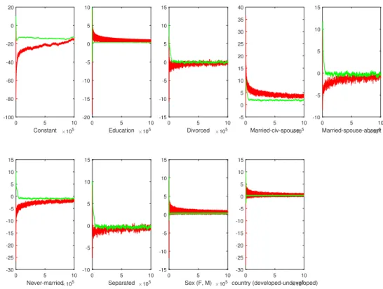
lines) methods for selected components ofθ, withm= 500, number of iterations 106. . . 46 5.2 The estimated values obtained by MH (green lines) and SGLD (red

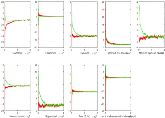
lines) methods for selected components ofθ, withm= 100, number of iterations 2×105_. _{. . . .} ₄₇ 5.3 The estimated values obtained by MH (green lines) and SGLD

(red lines) methods for selected components of θ, withm = 1,000, number of iterations 105. . . 47 5.4 The estimated values obtained by MH (green lines) and SGLD

(red lines) methods for selected components ofθ, whenm = 1,000, number of iterations 5×105_{. . . .} ₄₈ 5.5 Histograms of selected components of θ, obtained by MH (first

three lines) and SGLD methods (last three lines) withm = 10,000, number of iterations 105. . . 48 5.6 The estimated values obtained by MH (green lines) and SGLD (red

lines) methods for selected components of θ, with m = 10,000, number of iterations 105_{. . . .} ₄₉ 5.7 The posterior means of the components, obtained by MH (*) and

SGLD (o) and complete case (+) algorithms, with m = 500, num-ber of iterations 106. . . 50 5.8 The posterior variances of the components, obtained by MH (*)

and SGLD (o) and complete case (+) algorithms, with m = 500, number of iterations 106_{. . . .} ₅₁

(11)

LIST OF TABLES

3.1 Adult data for income level, ’ ?’ represents the missing parts . . . . 18 4.1 Comparison of MH and SGLD algorithms when subsample size is

100 (synthetic data). . . 34 4.2 Comparison of MH and SGLD algorithms when subsample size is

500 (synthetic data). . . 34 4.3 Comparison of MH and SGLD algorithms when subsample size is

10,000 (synthetic data). . . 34 4.4 Comparison of MH, SGLD and exclude-missings algoritms, m =

500, with iteration number is 5×104. . . 36 4.5 Comparison of MH, SGLD and complete case analysis algoritms,

with m= 500, number of iterations 105. . . 36 4.6 Posterior mean and variance values of components obtained by the

three algorithms, when subsample size is 500, and number of itera-tions is 5×104 _{(synthetic data). . . .} ₃₇ 5.1 Comparison of MH and SGLD algorithms when subsample size is

100, categorical dataset. . . 45 5.2 Comparison of MH and SGLD algorithms when subsample size is

500 (categorical dataset). . . 45 5.3 Comparison of MH, SGLD and complete case analyis algorithms

when subsample size is 1,000, categorical dataset. . . 52 5.4 Comparison of MH, SGLD and complete case analysis algorithms

(12)

LIST OF ALGORITHMS

1 Metropolis-Hastings . . . 8

2 Gibbs Sampling . . . 10

3 Metropolis-Hastings within Gibbs . . . 11

4 SGLD . . . 14

5 Metropolis-Hastings with Missing Data . . . 22

(13)

LIST OF SYMBOLS

A The masking matrix

exp Power of the natural exponential constant e

log Natural logarithm

N Number of samples

N(µ, σ2₎ _{Gaussian distribution with mean} _µ_{and variance} _σ2

p(·) Probability density function

t Iteration index in algorithms

q(·|·) Conditional density of proposal kernel

Y The output of models

Step size of SGLD algorithm

µ Mean vector of the probability distribution

η The noise vector

πi(·|·) Conditional distribution of ith component

Σ Co-variance matrix of probability distribution

(14)

LIST OF ACRONYMS/ABBREVIATIONS

i.i.d Independent and identically distributed

CCA Complete Case Analysis

MCMC Markov chain Monte Carlo

MH Metropolis-Hastings

PA Prediction accuracy

(15)

1. INTRODUCTION

Missing data [1] is a problem that occurs in almost all empirical research. The main concern is that, if the data were complete, would the results of the research be different [2, 3]? This question does not have an obvious answer, since incompleteness causes a decrease in the performance of parameter estimation and sensitivity of the method. If the missing data pattern is nonrandom, there is an additional concern that arises from bias. In this context, bias results in the failure of observed data to represent the incomplete parts [2]. In recent years, the interest in handling missing data mechanisms has increased and different techniques are introduced [4].

In the literature, there are various strategies to handle missing data problem [5]. The first approach, called listwise deletion (or complete case analysis), proposes to consider only observed variables, and do the calculations through the available parts of the data [6]. Although this idea is easy to implement, it loses the track of the un-available parts as well as ignores the possible differences between the characteristics of the observed and unobserved parts of the data. The second approach proposes the single imputation idea in which the missing components are replaced by the mean of observed variables. Since single imputation cannot reflect the uncertainty of imputa-tions, Rubin (1987) have introduced the multiple imputation idea, where all possible values for the latent variables are evaluated, and each one of them is used in parameter estimation [2, 5, 7].

Another well-known missing data handling technique is Expectation Maximiza-tion (EM). The foundaMaximiza-tions of EM framework is first laid down by Little and Ru-bin [8]. In this technique, maximum likelihood estimates are calculated for incomplete data [5]. As the name implies, the EM algorithm consists of two steps: Expectation and Maximization. The first (expectation) step calculates the conditional log-likelihood expectation of the observed data, when the observed data and the first parameter esti-mations are given, while the second step calculates the maximum log-likelihood of the expectation yielded by the first step, in order to obtain the parameter updates. The

(16)

cycle of expectation and maximization continues iteratively, until the convergence is attained [2].

1.1. Motivations and Contributions of the Thesis

This thesis investigates the Bayesian methods for incomplete data problems. Our motivation is to utilize the Metropolis-Hastings (MH) and Stochastic Gradient Langevin Dynamics (SGLD) methods in order to address incomplete data problems in large-scale datasets. The main contribution of this thesis is as follows: We have shown that using gradient estimates instead of the exact sampling methods [9,10] provides an efficient way to handle missing data. In SGLD framework, a Bayesian learning is iter-atively performed from large-scale datastes via small mini-batches. The mini-batches are used to approximate gradients and then the parameter updates are generated using the gradient information. Since the algorithm does not require computations over the whole dataset, a significant amount of time has saved, especially when the data size becomes larger. Another contribution of the thesis is to use MH sampling to replace latent variables in the dataset. MH [11, 12] is an efficient sampling method which en-ables us to draw samples for the cases where the full conditional distributions are not easy to sample from.

We introduce two approaches to the literature: The first approach uses MH idea for parameter estimation, whereas the second approach uses the SGLD idea. We have compared the performances of the algorithms, as well as we compare these methods with a method that proposes to consider only observed variables. The similar results are obtained by the implementations of three algorithms, and one can prefer one of them considering the advantages and disadvantages of the methods according to her preferences.

1.2. Scope of the Thesis

Chapter 2 provides a theoretical background for the readers. First the sampling problem is stated, then the Bayesian inference and the Markov chain Monte Carlo

(17)

methods are introduced. Chapter 3 introduces the incomplete data problem. The existing ways of handling this problem, especially in big datasets, are provided. This chapter concludes by proposing two MCMC-based methods to handle the incomplete data problem in big datasets. In Chapter 4, numerical results of the two proposed algorithms and a listwise deletion (or complete case analysis) algorithm on a Gaussian distributed synthetic incomplete dataset are shown with the methodology. Similarly, in Chapter 5, the proposed methods and complete case analysis method are applied on a real dataset, the methodology and results are also given. Finally, in Chapter 6, the results are discussed and possible future works are suggested.

(18)

2. MARKOV CHAIN MONTE CARLO METHODS

Markov chain Monte Carlo (MCMC) methods are mostly used to approximate the probability densities by a finite number of samples. Through this method, one can characterize a distribution even though the mathematical properties and the param-eters of the distribution are not completely known. As the name implies, an MCMC method is the combination of Monte Carlo and Markov chain approaches. Monte Carlo is the part where properties of a distribution is estimated by drawing samples and ex-amining them, while Markov chain part provides the memorylessness property in which each new sample depends only on the one before it [13].

An MCMC method depends on an ergodic Markov chain whose stationary distri-bution isπ. If an ergodic Markov chain with stationary distributionπ is simulated for long enough time, it will converge toπ. This convergence property makes it possible to sample the estimated parameters from a Markov chain with the stationary distribution being the target distribution π [14].

2.1. The Sampling Problem

Let us suppose we have N random samples X(1:N) ₌_X(1)_{, X}(2)_{, ..., X}(N) _{from a} set X. The samples are independent and identically distributed with respect to some unknown probability distributionπ. We can notate this as

X(1), X(2), ..., X(N)i.i.d.∼π.

Although the probability distribution P is unknown, we can approximately calculate its mean value (the expectation of X) via these samples X(1:N). The expectation can be written as

Eπ(X) =

Z

X

(19)

where π is also used as the probability density function of π. An approximation for this expression is given as

Eπ(X)≈ 1 N N X i=1 X(i). (2.2)

We can modify (2.2) for a certain function ϕof X with respect to π:

Ep(ϕ(X))≈ 1 N N X i=1 ϕ(X(i)). (2.3)

One can calculate (2.3) without knowing anything explicitly about π. The samples

X(1:N) _{are sufficient to evaluate the integral.}

However, if we know about P but we are not given any samples from it, then we cannot calculate the integral in (2.3). In order to handle this problem and estimate (2.3), we can generate our own samples fromπ. The main idea behind the Monte Carlo methods is that we can avoid the implementation ofπ if we generate samples from it.

2.2. Bayesian Estimation

Bayesian parameter estimation which gives weight to prior knowledge and reweights it with the available data, is an example where sampling methods are used. In Bayesian estimation the distribution of interest is π(x) =p(x|y), the conditional distribution of the unknown parameter given the observed variabley.

p(x|y) = p(x)p(y|x)

p(y) , (2.4)

Here, p(x|y) is the posterior probability density, p(x) is the prior probability density and p(y|x) is the likelihood function. Since p(y) does not depend on the variable of interest x, in Bayesian literature it is usually neglected and (2.4) can be written as

(20)

In simple words, the Bayesian idea is

posterior distribution∝prior distribution×likelihood function

The expression in (2.5) consists of the prior densityp(x), which is an estimated descrip-tion of where the parameters are located before the data is analyzed, and the likelihood

p(y|x) which represents the modelling of the data [15]. The Bayesian framework states that a posterior distribution that contains all available knowledge about parameters can be constructed when prior information is shaped by the available data, i.e. the likelihood function [16]. In this thesis, the likelihood function is chosen from regression models to make parameter estimations from the observed data.

2.3. MCMC Methods

Markov chain Monte Carlo is a generic method to draw samples of x from ap-proximate distributions and correcting these samples to obtain better approximations for the target distributionπ. The samples come sequentially, in which the distribution of last sample depends on the previous one. Thus a Markov chain is formed by these samples.

The idea behind MCMC is to construct a Markov chain whose stationary distri-bution is π and simulate it long enough time that the distribution of current samples converge to the target distribution. The convergence of MCMC methods has been proven in the literature, even though the samples generated from the Markov chain are not independent and identically distributed. MCMC methods are mostly used in applications where there are intractable densities which are approximated by finite number of samples [12].

Let us suppose that the probability distribution of state is denoted by π(t)₍_x_{) at} iterationt. The objective is to build a Markov chain such thatπ(t)(x) converges to the target distributionπ, ast goes to infinity. We need to specify a transition probability

(21)

chain at iteration t+ 1 is calculated as

π(t+1)(x0) = Z

x

π(t)(x)T(x0;x)dx. (2.6)

There are several requirements that we need to satisfy when designing an MCMC method. The first one is that the desired distribution should be an invariant distribu-tion of the Markov chain. The second condidistribu-tion states that the Markov chain should be ergodic. The chain should be aperiodic and irreducible to provide ergodicity.

One way to ensure the invariance of the target distribution is to show that the detailed balance property holds for the transition kernel. The detailed balance property is given as [17]:

T(xa;xb)π(xb) =T(xb;xa)π(xa), ∀xa, xb ∈ X.

2.3.1. Metropolis-Hastings Method

The Metropolis-Hastings algorithm is a well-known MCMC method devised by Metropolis and Ulam [18] and improved by Hastings [19].

The algorithm uses a Markov transition kernel q on X, in order to propose new values from the old ones. The proposal values, x0, are chosen from these simpler proposal distributions, often in the neighborhood of current parameters, x.

The algorithm draws a starting pointx0 from a starting distribution which might be based on an approximation. Then for every iteration t, a new value x0 is proposed by sampling from the proposal distribution q, i.e. x0 ∼q(·|x(t−1)_{). The proposed value}

(22)

is accepted as the new value of x, with the acceptance probabilityα(x, x0) where α(x, x0) = min 1,π(x 0₎_q₍_x_|_x0₎ π(x)q(x0_|_x₎ , x, x0 ∈ X.

If the proposal is accepted, then the algorithm sets the value of x(t) as x0, and if the proposal is rejected the algorithm sets the value of x(t) _as_x(t−1)_{. Even if the proposal} value is rejected at iteration t, it is still counted as an iteration. Given the current value x(t−1)_{, the transition kernel} _q

t(x(t)|x(t−1)) of the Markov chain is a combination

of a point mass at x(t−1) = x(t), and a weighted version of the proposal distribution

q(x(t)_|_x(t−1)_{), which adjusts the acceptance probability [12]. Algorithm 1 shows the} steps of the Metropolis-Hastings method.

The ratio in the acceptance probability α is called the acceptance ratio or accep-tance rate:

r(x, x0) = π(x

0₎_q₍_x_|_x0₎ π(x)q(x0_|_x₎.

If the proposal distributions are equal, i.e. q(x|x0) = q(x|x0), then the algorithm is called Metropolis method.

Algorithm 1 Metropolis-Hastings

1: Begin with somex0 ∈ X

2: for t= 1,2, ..., N do 3: Samplex0 ∼q(x0|x(t−1)₎

4: Set x(t)=x0 with probability

α(x(t−1), x0) = min 1, π(x 0₎_q₍_x(t−1)_|_x0₎ π(x(t−1)₎_q₍_x0_|_x(t−1)₎ , 5: Else set x(t) ₌_x(t−1)_. 6: end for

(23)

2.3.2. Gibbs Sampling

The Gibbs framework is one of the most well known MCMC sampling methods, which can be used when the the random variable X is multi-dimensional. The idea behind the method is drawing samples from complete (or full) conditional distributions sequentially, thereby producing a Markov chain by updating one parameter at a time with the posterior density as its stationary distribution [20]. The foundations of Gibbs sampling idea were laid down by Stuart Geman and Donald Geman, and its name was dedicated to physicist J. W. Gibbs due to the similarities between sampling algorithm and the statistical physics [17].

Let X = (x1, x2, ..., xd) be a random variable (vector) with density π(X) = π(x1, ..., xd). Assume further that one can sample for π(x) from the conditional

densi-tiesπi(xi|x1, ..., xi−1, xi+1, ..., xd),i= 1,2, ..., d, but not fromπitself. A successively

im-plemented Gibbs method will provide samples from the conditional densities π1, ..., πn

by conditioning on the latest samples.

The sampling procedure of the Gibbs sampling at iteration number t is given by the following: x(₁t) ∼π1(x (t−1) 1 |x (t−1) 2 , x (t−1) 3 , ..., x (t−1) d ) x(₂t) ∼π2(x (t−1) 2 |x (t−1) 1 , x (t−1) 3 , . . . , x (t−1) d ) .. . x(_dt) ∼πd(x (t−1) d |x (t−1) 1 , x (t−1) 2 , ..., x (t−1) d−1 ).

It is guaranteed that the samples come from the exact distributionP(x) as the number of iterations goes to infinity. Algorithm 2 shows the steps of the Gibbs sampling method.

(24)

Algorithm 2 Gibbs Sampling

1: Begin with someX0 ∈ X

2: for t= 1,2, ..., N do 3: for i= 1,2, ..., d do 4: Sample x(_it) ∼πi(·|x (t−1) 1 , ..., x (t−1) i−1 , x (t−1) i+1 , ..., x (t−1) d ). 5: end for 6: end for

Gibbs sampling can be considered as a special type of MH method [12], where the acceptance probability is always one.

2.3.3. Metropolis-Hastings within Gibbs

As we can see from the previous sections, Gibbs and Metropolis-Hastings algo-rithms can be used in various combinations in order to draw samples from the distri-butions that we cannot directly calculate. The simplest method is the Gibbs method in which direct samples are drawn from the conditional posterior distributions. On the other hand, MH algorithm is mostly used for the cases where the full conditional distributions are not tractable.

If, in a model, some of the conditional posterior distributions can be calculated directly, whereas some of them cannot be calculated, the Metropolis-Hastings within Gibbs idea is used to perform the sampling. The components are updated one at a time with Gibbs sampling method if possible, and with Metropolis-Hastings moves otherwise [12]. The Algorithm 3 provides the steps for Metropolis-Hastings within Gibbs method.

(25)

Algorithm 3 Metropolis-Hastings within Gibbs

1: for i= 1,2, ...N do 2: for i= 1,2, ..., d do

3: Update xi by a Metropolis-Hastings move that targets

πi(·|x1, ..., xi−1, xi+1, ..., xd)

4: end for

5: end for

2.3.4. Stochastic Gradient Langevin Dynamics

Stochastic Gradient Langevin Dynamics (SGLD) algorithm is an iterative sub-sampling based technique for Bayesian learning from large-scale datasets, first proposed by Welling and Teh (2011). The main idea of the SGLD algorithm is combining stochas-tic optimization algorithms, in which small mini-batches are used to approximate gra-dients, with Langevin Dynamics approach, in which the updates for the parameters are generated using the gradient information. Langevin dynamics introduces noise to the parameter updates that make the parameters converge to the samples from the full posterior distribution, while stochastic optimization provides an optimized likelihood and approximation to the Markov chain [21]. In general, the algorithm is a transition from stochastic optimization to a Bayesian method that samples from the posterior distribution.

Stochastic Optimization in SGLD. Letθ be the vector of parameters, and Y be the random varible whose dimensions n×d. We can define the posterior distribution of n data items, Y = (y1, y2, ..., yn), as p(θ|Y)≈p(θ) n Y i=1 p(yi|θ).

(26)

• A subset of m data items, Y(t) ₌_{_y(t) 1 , y

(t) 2 , ..., y

(t)

m} is provided for each iteration t,

• The parameters in the randomly selected subset are updated according to the following equation: θ(t+1) =θ(t)+ ∆θ(t), (2.7) ∆θ(t) = (t) 2 ∇logp(θ (t)_{) +} n m m X i=1 ∇logp(y(_it)|θ(t)) ! . (2.8)

where t is the step size and its choice has an important role to ensure convergence.

The constraints that step sizes are required to meet are:

∞ X t=1 (t) =∞, ∞ X t=1 ((t))2 <∞. (2.9)

The parameters can attain the high probability regions without considering their ini-tialization through the first constraint, and it is guaranteed that they will converge to the point through second constraint [21].

Langevin Dynamics in SGLD. Langevin dynamics idea introduces a normally distributed noise term to the stochastic gradient optimization method. Adding appro-priate amount of noise term and choosing step-sizes that satisfy the conditions in (2.9) will ensure that the parameters will converge to the samples of the posterior distribu-tion. In order to obtain samples that come from the posterior, the gradient step-sizes and the variance of the noise term are matched. Injecting Gaussian noise into the parameter update given in (2.8) yields a new update:

∆θ(t) = (t) 2 ∇logp(θ (t)_{) +} n X i=1 ∇logp(y(_it)|θ(t)) ! +η(t), (2.10) where η(t) _{∼ N}₍₀_,(t)_).

(27)

Since Langevin dynamics simply aim to discretize a stochastic differential equa-tion with an equilibrium distribuequa-tion coming from the posterior, (2.10) can be con-sidered as a proposal distribution. Then Metropolis-Hastings decides whether this proposal is accepted or rejected to correct the error arisen from the discretization [21]. Another method that corrects the discretization error is Hamiltonian Monte Carlo where Metropolis-Hastings framework is still applied, but instead of coming from a random walk, the proposals are chosen such that they enable more efficient transitions between the states via the momentum variables [23].

Combining SG with LD. The stochastic gradient optimization provides estimates for the gradient information using a subset of the dataset, without considering the un-certainty, while Langevin dynamics approach handles with the parameter uncertainty and data over-fitting problems processing the whole dataset. Combining the expedient properties of these two techniques helps improve the performance of the parameter estimation, especially when we have a large-scale dataset. SGLD framework provides Bayesian learning from huge datasets using small mini-batches iteratively. The pa-rameter update of SGLD algorithm which is a combination of (2.8) and (2.10), is the following: ∆θ(t) = (t) 2 ∇logp(θ (t)_{) +} n m m X i=1 ∇logp(y(_it)|θ(t)) ! +η(t), (2.11)

where η(t) _{∼ N}₍₀_,(t)_{) and the step-sizes satisfy (2.9), i.e. converge to zero.}

The decay of step-sizes makes the rejection ratio of MH close to zero. Thus we do not need to go over the whole dataset and calculate the probabilities to obtain acceptance ratios of Metropolis-Hastings algorithm.

(28)

Algorithm 4 SGLD

1: Input: a, b, γ

2: for t= 1,2, ..., T do

3: Choose a random subset of m data items y(t)_{= (}_y(t) 1 , ..., y

(t)

m)∈Y

4: Calculate the step size

(t) =a(b+t)−γ and η(t) ∼ N(0, (t)), 5: Set θ(t+1) =θ(t)+ (t) 2 ∇logp(θ (t) + n m m X i=1 ∇logp(y(_it)|θ(t))) ! +η(t) 6: end for

(29)

3. MISSING DATA PROBLEMS IN REGRESSION

MODELS

3.1. Regression Models

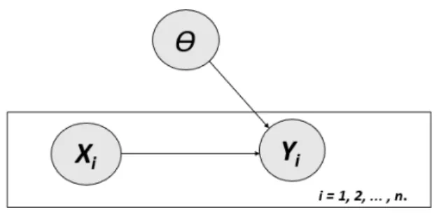
Regression is a method of modelling a target value based on independent predictor values, mostly used for explaining the causal relationship between the variables. The number of independent and dependent random variables, and the type of relationship between them are the two factors that determine the regression technique [12]. A simple structure of a regression model is depicted in Figure 3.1.

Figure 3.1: Schematic of a Regression Function.

3.1.1. Linear Regression

Linear regression is a simple regression analysis where there is one independent random variable which is linearly related to the dependent variable. In linear regression, input and output values are both numeric.

The linear equation assigns one scale factor to each input value (or column) called coefficient. An additional coefficient that gives one more degree of freedom is added. The added coefficient is often called the bias coefficient that helps move the model up

(30)

or down. A generalized linear regression model is defined as

y=Xθ+,

wherey = (y1, y1, ..., yn)Tis ann×1 dependent variable (output) vector,X is the

inde-pendentn×drandom variable (input) matrix,θ = (θ1, θ2, ..., θd)T are the corresponding coefficient values of X, and is an n-dimensional error term.

The model for predicting a single component, say ith _{component, of} _X _{can be}

written as

yi =xiθ+i, (3.1)

where yi is a scalar value, ith element of y, xi = (xi,1, xi,2, ..., xi,d) is a 1×d vector (ith

row ofX), and i is the corresponding scalar value of error term [24].

The aim of learning a linear regression model is to estimate the values of coef-ficients used to represent the available data. There are various estimating methods based on the dimension of the variables, such as ordinary least squares and gradient descent.

3.1.2. Logistic Regression

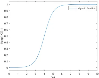
Logistic regression is a binary classification method that measures the relationship between a binary dependent variable and one or more independent variables. The dependent variable is restricted to binary values, while independent variables can be continuous. Logistic regression model, which uses the sigmoid function to estimate the probability of occurrence of an event for a single variable, is defined as

p(yi = 1|xi, θ) =

1

(31)

where yi is the binary response variable (or outcome of an event), and xi is the ith

row ofX given in Section 3.1.2, and θ = (θ1, θ2, ..., θd)T is the parameter vector of the

logistic regression model [25]. The graph of sigmoid function and visual representation of logistic regression model is depicted in Figure 3.2.

0 1 2 3 4 5 6 7 8 9 10 X 0 0.1 0.2 0.3 0.4 0.5 0.6 0.7 0.8 0.9 1 1/exp(-X )+1 sigmoid function

Figure 3.2: Graph of a Logistic Regression Function.

Logistic regression modelling is a widely-used and efficient technique since it does not require too many computations or input features to be scaled as well as it is easy to interpret. On the other hand, logistic regression can be applied only on the data which already has clearly identified independent variables. It is also vulnerable to over-fitting, which is the problem of failing to represent additional components of the data, due to the production of a rule that extremely corresponds to a particular set of data [26, 27].

3.2. Missing Data

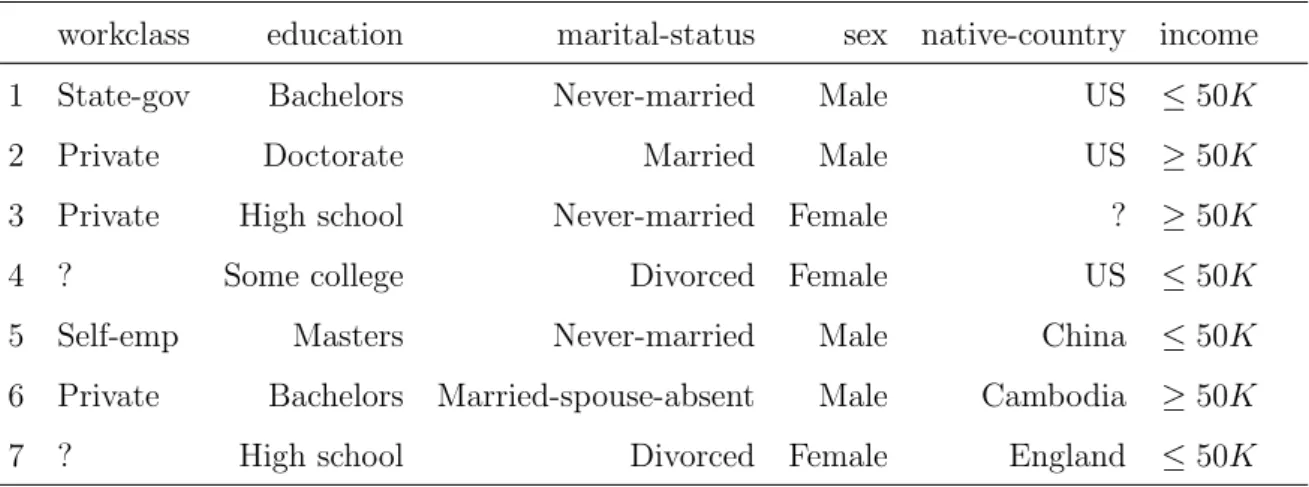
Incomplete data problem may arise naturally or intentionally. The dataset can contain latent variables because of the design of the researcher or noncompliance of respondents [7]. As an example, portion of a census data, which aims to predict whether a person’s income exceeds $50,000 per year or not, with some missing values is shown in Table 3.1. Since incompleteness increases the complexity of the data analysis, studies have been conducted to analyze the missing data patterns deeply, and understand

(32)

their effects on the results of regression models. Incompleteness patterns are basically categorized into two: missing at random and missing at nonrandom. The nonrandom pattern may cause the additional problem of bias, which is the failure of observed data to represent the unobserved parts of the data. Thus, it is more difficult to handle [2].

workclass education marital-status sex native-country income 1 State-gov Bachelors Never-married Male US ≤50K

2 Private Doctorate Married Male US ≥50K

3 Private High school Never-married Female ? ≥50K

4 ? Some college Divorced Female US ≤50K

5 Self-emp Masters Never-married Male China ≤50K

6 Private Bachelors Married-spouse-absent Male Cambodia ≥50K

7 ? High school Divorced Female England ≤50K

Table 3.1: Adult data for income level, ’ ?’ represents the missing parts

3.3. Previous Methods in Literature

The first proposed procedure for handling missing data is excluding the missing components of the data and using only the observed ones. Although this procedure is easy to implement, it loses the information of incomplete cases. Since the approach ignores the possible differences between missing and observed parts of the data, the resulting inference may fail to reflect the complete dataset. Another approach proposes to substitute a predicted value for each missing component in dataset. For example, the mean of observed components can be used to replace the missing values. The algorithm is called single imputation that applies standard statistical procedure to newly predicted complete dataset. Since single imputation performs as if there is no missing value in dataset, it cannot reflect the uncertainty of predictions for missing values, and it can produce biased resulting variances of estimated variables which tend to converge to zero [5]. Rubin [8] has proposed a strategy called multiple imputation. Multiple imputation procedure imputes each missing component with a set of possible values. Through these multiple values offered, the uncertainty of missing variables can be represented. The algorithm performs the standard data analysis procedure to each

(33)

filled dataset. Then it combines and compares the results for the inference.

3.3.1. Non-MCMC Methods

The non-MCMC procedures for handling missing data generally can be assorted into two categories which are regression-based and neighbor-based approaches [28].

A regression-based approach uses linear or logistic regression model to obtain missing variables. The missing variables are assumed as response variables (dependent variables), whereas the observed ones are assumed as predictor variables (independent variables). The strategy produces imputations which are defined as samples from pos-terior predictive distributions specified by the regression model. The iterative imputing procedure continues by overwriting previously sampled values [29].

A neighbor-based approach uses a certain distance function to predict the missing values in the data. The distance function is supposed to determine the closest vector in order to impute the missing vector. The closest vector is the one whose characteristics are similar to the incomplete vector [28, 30].

3.3.2. MCMC Methods

The main idea of MCMC approach to handling missing data is that the values are generated via a statistical model that describes the distribution of the complete data. An improved version of this approach uses Bayesian networks. A Bayesian network provides a natural way to encode the relations between and within the variables. In order to comprehend the theory behind the MCMC methods with Bayesian inference for handling missing data, it will be helpful to clearly provide the definition of posterior distribution using the prior and joint densities.

Suppose that we have ann×dmatrixX, that consists of observed and unobserved variables, such that X = (Xmiss, Xobs), its corresponding d-dimensional parameter vector for the given model is θ= (θ1, θ2, ..., θd)T, and the n-dimensional output vector

(34)

of the model is Y = (y1, y2, ..., yn)T. Using the Bayesian idea described in Section 2.1,

we can write the conditional probability of ofXmiss:

π(θ, Xmiss) =p(θ, Xmiss|Xobs, Y)∝p(θ, Xmiss, Xobs, Y) =p(θ)

n

Y

i=1

p(xmiss,i, xobs,i|θ)p(yi|xmiss,i, xobs,i, θ),

where we assume X is independent of θ,i.e.

p(xmiss,i, xobs,i|θ) =p(xmiss,i, xobs,i) = p(xi),

p(yi|xmiss,i, xobs,i, θ) =p(yi|xi).

The procedure starts with Bayesian learning for variables, and then an MCMC tech-nique is employed to draw samples from the probability distributions learned by the Bayesian network. The algorithm continues iteratively, until the convergence is reached. This method provides unbiased estimates, as well as the confidence levels of the impu-tation results [31].

Data Augmentation. Data augmentation is another traditional multiple impu-tation algorithm based on MCMC technique [32]. Parameter estimates are produced by repeating substitution conditionally on the prior value, constructing a stochastic process called Markov chain [33]. Suppose we have a dataset X = (Xmiss, Xobs), its parameter vector θ = (θ1, θ2, ..., θd)T and Y = (y1, y2, ..., yn)T, like in the previous sections. Then, the procedure of data augmentation algorithm can be written as

X_miss(t+1) ∼π(Xmiss|θ) = p(Xmiss|Xobs, θ(t), Y), (3.3)

θ(t+1) ∼π(θ|Xmiss) = p(θ|Xobs, X (t+1)

(35)

The imputation step is given in relation (3.3), where predicted values are generated from prior conditional distribution of missing values given the observed values and the parameter values at tth _{iteration. Relation (3.4) is the parameter update part, where}

parameter values are generated from the posterior distribution, given the observed values and replaced values of X at the (t + 1)th _{iteration. This procedure continues}

iteratively until its convergence is attained. The multiple imputation can be performed in two different ways. The first method runs a single chain for all iterations and takes every tth prediction for Xmiss, whereas the second method runs for parallel chains and takes the last values for replacing from these chainsXmiss [32].

Metropolis-Hastings for Imputation and Parameter Estimation. Here, we note a contribution to the approach described in the previous section for the cases, where the full conditional distributions are not easy to sample from. We propose to use Metropolis-Hastings idea for imputation of missing variables. Especially for the cases where drawing samples is not possible or computationally efficient, making MH moves and updating Xmiss will improve the performance of regression with missing data.

Suppose that X is the data matrix whose dimensions are n×d, which contains missing variables in it, and its parameter and outcome vectors are the same with the ones defined in Section 3.2. The proposed algorithm for imputing missing data and estimating parameters is as follows: At every iteration t, an inner loop performs to impute the missing values in ith row of X, where i = 1,2, ..., n, by making MH moves for latent variables, while θ is supposed to be fixed. The proposal values for missing variables are updated according to the acceptance ratio of MH algorithm. In the experiments we have conducted, we choose the kernel proposal distribution q as symmetric random walk. So, the q ratio for Xmiss is simply one. After the imputation period is completed in the inner loop, the provided X value is fixed and used to estimate parameters of the model. The algorithm estimates θ by MH moves again, using imputed version of X(t)_{. The proposal kernel distribution for} _θ _{is also chosen} as symmetric random walk giving the q ratio is one. This iterative process continues until convergence is obtained. Algorithm 5 shows the steps of the introduced method

(36)

for data augmentation and parameter estimation.

Algorithm 5 Metropolis-Hastings with Missing Data

1: Begin with someX(0) _{∈ X}

2: for t= 0,1, ..., T do 3: for i= 1,2, ..., n do

4: Sample x0_miss_,i∼q(x0_miss_,i|x(_misst) _,i)

5: Set x(_misst+1)_,i=x0_miss_,i with probability

α(x(_misst) _,i, x0_miss_,i) = min ( 1,π(xmiss,i|θ)q(x (t) miss,i|x 0 miss,i) π(x(_misst) _,i|θ)q(x0_miss_,i|x(_misst) _,i)

)

.

6: Else set x(_misst+1)_,i =x(_misst) _,i.

7: end for

8: Sampleθ0 ∼q(θ0|θ(t))

9: Set θ(t+1) ₌_θ0 _{with probability}

α(θ(t), θ0) = min ( 1, π(θ 0_|_X(t) miss)q(θ(t)|θ 0₎ π(θ(t)_|_X(t) miss)q(θ0|θ(t)) ) . 10: Else set θ(t+1) =θ(t). 11: end for

3.4. SGLD Method for Missing Data in Big Datasets

Unlike typical optimization-based methods where point-wise estimations for pa-rameters are aimed to obtain, Bayesian methods attempt to provide the full posterior distribution of parameters based on the available data and the prior distribution. In this way, better characterizations are obtained, and the uncertainty is captured. Even though Bayesian methods provide these advantages, they are not popular in large-scale machine learning problems. The main reason for that is that a typical Markov chain Monte Carlo algorithm requires computation over the entire dataset at each iteration.

(37)

such as internet traffic and network data or survey results have shown that Bayesian estimations is a feasible approach to handle the missing data problem. Ni and Leonard (2005) introduced the idea of using Markov chain Monte Carlo methods for sampling and imputing missing data [31], and then using the imputed data to estimate param-eters. Their experiments have shown that MCMC methods are successful to estimate parameters when the data is not complete.

We aim to utilize the advantages of MCMC methods for handling the incomplete data problem by introducing the SGLD framework. As it is mentioned before, the SGLD method provides learning from large-scale datasets based on iterative learning from small mini-batches. We propose a hybrid algorithm that combines the Metropolis-Hastings idea with SGLD. The hybrid algorithm makes an SGLD move forθ using an estimate of gradient log-likelihood of a randomly selected subsample, while taking MH steps for unobserved elements of X. The imputation of X is performed by an inner loop, where the latent variables in the subsampled matrix are imputed line by line. After the imputation period, the parameter estimation is performed via averaging the gradients calculated with completed X whose missing components are sampled with MH moves. The procedure of the MH-SGLD algorithm is outlined in the Algorithm 6.

Here we have a small notation change. In this context, let u denote the missing variables inith _{row of}_X_, _i.e._u₌_x

miss,i, andz denote the combination of the observed

variables inith row of X with the corresponding output, i.e. z = (xobs,i, yi). Then the derivations for the gradient of log-likelihood for incomplete data is calculated by the following:

∇logpθ(z) =

Z

(38)

where the gradient of pθ(u, z) is calculated as

∇logpθ(u, z) = ∇log(p(u)pθ(z|u))

=∇logp(u) +∇logpθ(z|u) =∇logpθ(z|u).

Since prior probability distribution ofu is independent ofθ, its derivative with respect toθ is zero. Thus, the second line is followed by the third line.

When exact sampling is not possible, MH can be employed to draw samples

u(1), u(2), ..., u(N)

frompθ(u|z) so that the gradient of log-likelihood is approximated as

∇logpθ(z)≈ 1 N N X i=1 ∇logpθ(u, z).

We have conducted some experiments in order to observe and compare the perfor-mances of two approaches that we propose. The imputation part given in (3.3) is the same for both MH and SGLD algorithms, whereas the parameter updates are differ-ent. The main question is: Can we obtain similar results with MH sampling, if we use gradient approximations of a small subset of the data for parameter estimations? In this way, we aim to enhance the performance of regression with missing data according to time and efficiency measures.

(39)

Algorithm 6 SGLD with Missing Data

1: Input: a, b, γ

2: Start with an initial value X(0) _{∈ X}

3: for t= 1,2, ..., T do

4: Choose a random subsample U ⊂ {1,2, ..., n} such that the size of U ism.

5: for u= 1,2, ..., m do

6: x(0)u =x(

t−1)

u

7: for j = 1,2, ..., J do

8: Updatex(_u,t,j_miss) →x(_u,t,j−_miss1) given (yu, xu,obs, θ)

9: Set x(ut,j)= (x_u,(t,j_miss) , x(_u,t)_obs)

10: end for 11: Calculate ∇logp(yu|x (t) u,miss, θ) = 1 J J X j=1 ∇logp(yu|x(ut), θ) 12: end for 13: Calculate (t) =a(b+t)−γ and η(t) ∼ N(0, (t)), 14: Set θ(t+1) =θ(t)+ (t) 2 ∇logp(θ (t)_{) +} n m m X i=1 ∇logp(yu|x(ut), θ (t)₎ ! +η(t) 15: end for

(40)

4. EXPERIMENTS WITH SYNTHETIC DATA

In this chapter, the applications of two proposed methods on an artifical dataset are presented. In addition to this, another missing data algorithm mentioned in Section 3.3 is implemented in order to compare the performances of proposed algorithms with an existing algorithm. Methodology and the derivations are also provided.

4.1. Data Description

We generate a data matrix X whose dimensions are n×d. The variables in X

has Gaussian distribution with mean and covariance parameters denoted byµxand Σx,

respectively. Since the aim is to measure the performances of algorithms for large-scale datasets, we choose n= 500,000 andd= 5. In order to obtain missing variables in X, we produce a response indicator matrix A with the same dimensions of X. We mask some random variables by pointwise multiplication ofXbyA, wheneverX is observed,

A is equal to one; otherwise A is equal to zero. The sparsity of A can be adjusted so that one can obtain different ratio of unobserved values to observed ones and observe the effect of missingness on parameter estimation. The n-dimensional output vector

Y is obtained by applying the logistic regression function to X and its given initial parameter vector. The parameter vector for logistic regression function is denoted by

θ= (θ1, θ2, ..., θd)T. It is supposed that the initial parameter vector is distributed from

normal distribution with mean and covariance denoted by µθ and Σθ accordingly.

4.2. Methodology

As it is stated in the previous chapter, the proposed algorithm completes unob-served parts of the data by making MH moves. Since we aim to introduce a framework that utilizes the Metropolis-Hastings and SGLD ideas, instead of the whole dataset, we work with the randomly selected subset ofX. The algorithm chooses a random subset at each iteration and completes the unobserved parts of only this subset. The algorithm assumes that the variables are independent and identically distributed. Therefore, we

(41)

can work with each element in a row separately, and we can suppose that replacing one element with a proposed value does not affect the probability of others.

4.2.1. Imputation of Missing Components

The imputation is necessary when the subsampled predictor matrix has missing values. The location of the missing variables in X is indicated by zeroes in a binary matrix, sayA, whose variables are 0 to represent missing components inX. We provide the prior parameters for X, and the algorithm performs Metropolis-Hastings move for the missing variables in the predictors of a logistic regression model.

We use the logarithmic values of prior conditional probabilities and proposal dis-tributions in order to make calculations conveniently. For our case, ratior(xmiss,i, x0miss,i)

in the acceptance probability α(xmiss,i, x0miss,i) is defined as

r(xmiss,i, x0miss,i) =

π(x0_miss_,i|θ)q(xmiss,i|x0miss,i) π(xmiss,i|θ)q(x0miss,i|xmiss,i) .

Theq ratio is one since proposal kernel is chosen as a symmetric random walk and the conditional probabilities are calculated by the Bayesian approximation. That is

0 i, θ),

where x0_i = (x0_miss_,i, xobs,i). So we obtain the acceptance ratio as

r(xmiss,i, x0miss,i) =

p(x0_i)p(yi|x0i, θ) p(xi)p(yi|xi, θ) .

(42)

Calculation of Prior Probability Ratio. The logarithmic ratio of prior probabil-ities of xmiss,i and x0miss,i can be defined as

logp(x

0

miss,i) p(xmiss,i)

= logp(x0_miss_,i)−logp(xmiss,i)

=−1 2 (x

0

miss,i−µx)Σ−1(x0miss,i−µx)T−(xmiss,i−µx)Σ−1(xmiss,i−µx)T

.

(4.1) The evaluation of the expression in (4.1) requires calculations for each row of X (xi)

separately, which means that we need to perform n operations in one iteration. In order to avoid deceleration in the algorithm caused by these row operations, we apply the Cholesky decomposition to the covariance matrix Σx. We can write Σx = CTC

where C is the Cholesky factor of Σx. If we represent (xmiss,i −µx) by Z, then the

logarithm of the prior probability ratio can be expressed as

log p(x 0 miss,i) p(xmiss,i) + =−1 2(ZC −1₎₍_ZC−1₎T_, _(4.2)

which can be evaluated by taking the square of product of two matrices, instead of evaluating each row ofXmiss individually.

Calculation of Likelihood Ratio. The second part of the acceptance rate is the ratio of logistic regression functions evaluated at the current and the proposed values for X. Again we take the logarithm, and define the likelihood ratio vector as

logp(yi|x 0 i, θ) p(yi|x0_i, θ) = logp(yi|x 0 i, θ)−log(p(yi|xi, θ). (4.3)

We plug the logistic regression function, and after simple calculations, obtain the like-lihood vector as logp(yi|x 0 i, θ) p(yi|xi, θ) =−(x0_i−xi)θ(1−yi)−log(1 +e−x0iθ_{) + log(1 +}_e−xiθ₎_. _(4.4)

(43)

Obtaining the ratio vectors defined in (4.1) and (4.4) and taking the summation of them yield the logarithm of the acceptance rate. The algorithm updates missing variables ofX according to this acceptance rate in an inner iteration that we call burn-in. Thus the first imputations for Xmiss are discarded and more reliable replacements are presented. The sampling of missing variables in Xmiss is completed at this point.

4.2.2. Parameter Update Using MH

After sampling and replacing missing X components for each iteration, we es-timate the parameter θ when we suppose that X and Y are given. We propose a value for next value ofθ that also comes from random walk and calculate the ratio of conditional densities as π(θ0|X) π(θ|X) = p(θ0)Qn i=1p(yi|xi, θ 0₎ p(θ)Qn i=1p(yi|xi, θ) ,

where θ0 = θ +z is the proposed value of θ, and z ∼ N(0,Σq) is the random walk

step with zero mean and variance Σθ. Since proposal kernel is symmetric random

walk, q ratio is one again. We apply the same procedure with X, which is taking the logarithms and calculating prior probability ratio vector and likelihood ratio vector separately. Then, the combination of these vectors provide acceptance probability vector of MH algorithm for parameter update.

Since θ is supposed to be normally distributed with mean µθ and covariance Σθ,

we can calculate the logarithm of its prior probabilities as

log p(θ 0₎ p(θ0₎ = logp(θ 0₎₋_log_p₍_θ₎ = loge−0.5(θ0−µθ)Σ−θ1(θ 0_−µ θ)T −loge−0.5(θ−µθ)Σ−θ1(θ−µθ)T =−0.5(θ0−µθ)Σ−θ1(θ 0₋ µθ)T+ 0.5(θ−µθ)Σθ−1(θ−µθ)T. (4.5)

(44)

The log-likelihood ratios for parameters of the logistic regression function is

log p(yi|xi, θ

0₎ p(yi|xi, θ)

= logp(yi|xi, θ0)−logp(yi|xi, θ) =−(θ0−θ)xi(1−yi)−log(1 +e−xiθ

0

) + log(1 +e−xiθ₎_, _(4.6)

4.2.3. Parameter Update Using SGLD

The first part of the algorithm provides a complete subset of the data that we use to estimate the parameters for the logistic regression model. In this second part of the method, incompleteness is not considered and the algorithm makes an SGLD move forθusing an approximate value of gradient log-likelihood of a randomly selected subsample. The gradient estimation is performed via averaging the gradients calculated with complete X, whose missing components are sampled with MH moves.

The algorithm first calculates the estimates for gradient of prior distribution, which is the first part of (2.11). In order to make calculations more conveniently, we prefer to use the logarithmic values of priors. Since we have normally distributed parameter vector, we define its gradient of log-prior as

∇θlogp(θ) = ∇θlog e−12(θ−µθ) T_Σ−1₍_θ−µ θ) =∇θ −1 2(θ−µθ) T_Σ−1₍_θ₋_µ θ) =−Σ−_θ1(θ−µθ). (4.7)

(45)

probabilities. The sum-log-posterior is derived by the following: m X i=1 ∇θlogp(yi|xi, θ) = m X i=1 ∇θlog e−xiθ(1−yi) 1 +e−xiθ = m X i=1 ∇θ −xiθ(1−yi)−log(1 +e−xiθ) = m X i=1 −xi(1−yi) + e−xiθ 1 +e−xiθ , (4.8)

where m denotes the sub-sample size.

Now, we need to introduce an appropriate amount of noise term to guarantee that the obtained θ values will converge to samples from true posterior distribution. The stepsize parameters are adjusted so that the noise term satisfies the required condition. The stepsize also needs to obey the convergence itself, and it is restrained by the constraints given in (2.9). The definitions of stepsize and noise term for each iteration t are

t =a(b+t)−γ and ηt ∼ N(0, t),

where a, b and γ are the stepsize parameters. Combining the gradient of log-priors (4.5), and the summation of log-posteriors (4.8), and adding the Gaussian noise term we obtainθ update within (3.4) as

∆θt = t 2 −Σ −1 θ (θ−µθ) + n m m X i=1 −xi(1−yi) + e−xiθ 1 +e−xiθ !! +ηt. (4.9)

4.3. Experiments and Results

The Gaussian data matrix is synthetically generated in the MATLAB environ-ment to test the algorithm on a normally distributed dataset with latent variables. The prior parameters, mean and covariance of the data are also provided. Then

(46)

an-other binary matrix whose dimensions are the same with the data matrix is generated in order to mask some variables in the dataset randomly. The zero values represent the latent variables in X, while one represents the observed variables. The sparsity of mask matrix can be adjusted so that the portion of incompleteness is determined. We also suppose that, for starting values, the parameter θ of the logistic regression model comes from normal distribution with specified mean and covariance values. The subsample size is denoted by m. The specified dimensions and the parameters are as follows:

• Data matrix Xn×d, with n = 500,000 and d= 5, • Mask matrix An×d, with n = 500,000 and d= 5,

• 20% of A is 0, meaning that 20% of the data is missing,

As we mentioned before, the data is fitted to the logistic regression function which is provided in (3.1), and the obtained results are compared by the prediction analysis. The steps of our prediction analysis are as follows:

• Separate the data into two sets: training and test,

• Use the training set to impute missing values and estimate parameters and ob-served components of test set,

• Determine the observed variables in the test set,

• Calculate the expected value of the likelihood function applying the expression given in (2.3) to the observed variables in the test set:

Ep(yi)≈ 1 N N X i=1 1 1 +e−xiθ(i) ,

where N is the number of iterations after burn-in period, and _Ep(yi) is the

pre-diction probability that determines the predicted value for yi.

• If the prediction probability is greater than threshold, which is chosen as 0.5 in our experiments, then assign the predicted value of the component to one, otherwise assign it to zero.

(47)

• Obtain the number of components where predicted value and actual value match, and calculate the total prediction accuracy by taking the ratio of the number of matching components to total number of components.

We have simulated MH and SGLD algorithms with different iteration numbers and subsample sizes. In order to reduce the computational costs in the MH algorithm, we use the same subsamplemwhen imputing latent variables inX, instead of using the whole dataset. On the other hand, when estimating parameters we sampled from the entire but partially-imputed dataset X. The results are compared according to their prediction successes and run times of the algorithms, when the iteration numbers are the same. However, we should point out that SGLD algorithm performs an additional inner loop to take the average of the estimated gradients. We choose the iteration number of inner loop as five and the burn-in period as three, in order to discard the first imputed missing values.

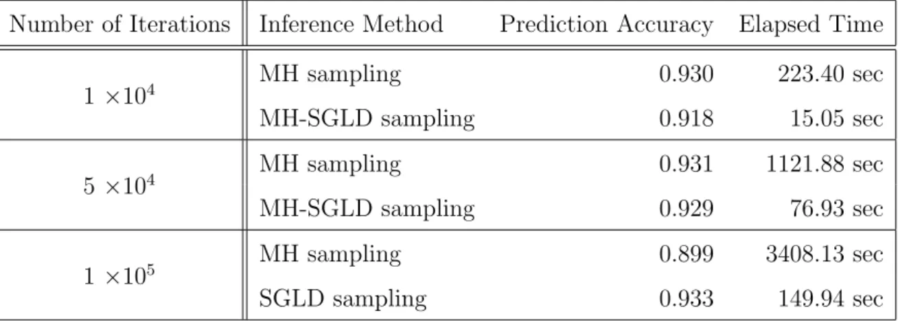
Table 4.1 shows the prediction accuracy for MH and SGLD results. It can be clearly seen that the iteration number does not have a great impact on the results when the subset size is 100, whereas the runtimes for these iteration numbers differ significantly for the algorithms. Approximately 92% of the obtained results for both MH and SGLD algorithms are consistent with the output which comes from the logistic regression model and its initial parameters. As the iteration number is increased, the prediction accuracy presented by the SGLD method starts to be greater than the prediction accuracy presented by the MH method.

Since the generated data has 500,000 samples, a subset of size 100 might not be enough to represent the entire data. So we have also run the algorithms with random subset of size 500 (0.1% of the data). It can be observed from Table 4.3 that the prediction accuracy has increased to 94% for the SGLD algorithm. The difference between the execution times of the algorithms is also increased, so one can prefer to apply SGLD algorithm instead of MH, especially when the data size becomes larger.

(48)

Table 4.1: Comparison of MH and SGLD algorithms when subsample size is 100 (synthetic data).

Number of Iterations Inference Method Prediction Accuracy Elapsed Time

1×104 MH sampling 0.930 223.40 sec MH-SGLD sampling 0.918 15.05 sec 5×104 MH sampling 0.931 1121.88 sec MH-SGLD sampling 0.929 76.93 sec 1×105 MH sampling 0.899 3408.13 sec SGLD sampling 0.933 149.94 sec

Table 4.2: Comparison of MH and SGLD algorithms when subsample size is 500 (synthetic data).

1 ×104 MH sampling 0.930 227.30 sec SGLD sampling 0.929 22.86 sec 5 ×104 MH sampling 0.929 1103.32 sec SGLD sampling 0.929 114.61 sec 1 ×105 MH sampling 0.870 3420.21 sec SGLD sampling 0.940 243.77 sec

Table 4.3: Comparison of MH and SGLD algorithms when subsample size is 10,000 (synthetic data).

1 ×104 MH sampling 0.954 396.35 sec SGLD sampling 0.954 75.88 sec 5 ×104 MH sampling 0.955 1948.72 sec SGLD sampling 0.955 355.60 sec 1 ×105 MH sampling 0.961 6003.84 sec SGLD sampling 0.955 712.61 sec

(49)

Figure 4.1: Histograms of parameter components of θ estimated by MH (above) and SGLD (bottom) withm = 500 and number of iterations 5×104.

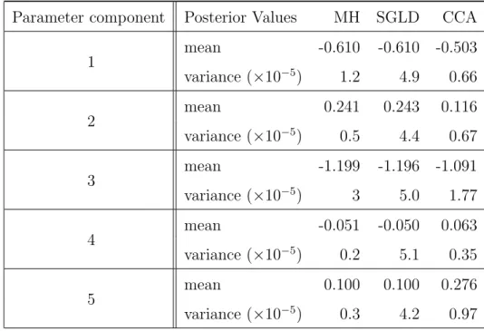
Figure 4.1 shows the histograms of five components of θ, when the subsample size is 500 and the number of iterations is 5×104_{. The histograms lying in the above} row are obtained by the MH algorithm, and the histograms lying in the bottom row are obtained by the SGLD algorithm. It can be observed from the figure that, the histograms obtained by the SGLD algorithm are narrower than the histograms obtained by the MH algorithm. Considering the variances of components provided in Table 4.6, where the components obtained by SGLD have higher variances, the difference between the histograms is as expected. Increasing the number of iterations might decrease the variances yielded by SGLD, and broader histograms similar to MH can be obtained.

In order to evaluate the performances of algorithms not only compared to each other, but also compared to the existing algorithms in the literature, we conducted experiments with the complete case analysis method in which the latent variables are excluded (mentioned in Section 3.3). We have observed the change in the prediction successes with the percentage of missing variables in the dataset. The simulations are run for 5×104 iterations, and the subsample size for SGLD algorithm is chosen as 500. In this third method, the MH algorithm is simulated using only with the observed components, and the resulting prediction successes are shown in Table 4.4. Clearly,

(50)

Table 4.4: Prediction Value for algorithms, withm= 500, number of iterations 5×104_. Missingness ratio PA for MH PA for SGLD PA for CCA

10% 0.946 0.941 0.895

20% 0.930 0.929 0.845

30% 0.930 0.874 0.814

40% 0.923 0.870 0.777

50% 0.892 0.868 0.731

Table 4.5: Prediction Value for algorithms, withm = 500, number of iterations 105_. Missingness ratio PA for MH PA for SGLD PA for CCA

10% 0.946 0.943 0.926

20% 0.932 0.940 0.900

30% 0.930 0.905 0.871

40% 0.922 0.872 0.820

50% 0.892 0.868 0.787

one can interpret that the three approaches have similar prediction values for small amount of latent variables. However, the success rate of the complete case analysis algorithm has significantly decreased when the ratio of missing variables gets higher. This might be caused by the lack of information of incomplete cases, as mentioned in Section 3.3. It can be stated that MH and SGLD algorithms have more tolerance to change in the ratio of incompleteness.

Table 4.5 provides the experiment results yielded by the three algorithms, with 105 _{iterations and a subsample size of 500. The aim of the tests with higher number of} iterations is to see the effect of iteration number on the success of complete case analysis approach. Even though the iteration number has raised the prediction accuracy, the algorithm is still outperformed by MH and SGLD algorithms, especially for higher rates of latent variables.

(51)

Table 4.6: Posterior mean and variance values of components obtained by the three algorithms, when subsample size is 500, and number of iterations is 5×104 _(synthetic data).

Parameter component Posterior Values MH SGLD CCA

1 mean -0.610 -0.610 -0.503 variance (×10−5₎ _1.2 _4.9 _0.66 2 mean 0.241 0.243 0.116 variance (×10−5₎ _0.5 _4.4 _0.67 3 mean -1.199 -1.196 -1.091 variance (×10−5₎ ₃ _5.0 _1.77 4 mean -0.051 -0.050 0.063 variance (×10−5₎ _0.2 _5.1 _0.35 5 mean 0.100 0.100 0.276 variance (×10−5₎ _0.3 _4.2 _0.97

(52)

5. EXPERIMENTS WITH REAL DATA

In this chapter, the proposed methods are applied to a real dataset, and the results are presented. In addition to this, another missing data approach is implemented in order to compare the performances of proposed algorithms with an existing algorithm. Methodology and the derivations are also provided.

5.1. Data Description

We analyze a real adult dataset that predicts whether the annual income of a person exceeds $50K or not based on the census data. The census data has various categorical variables that might affect the income level of adults such as education level, sex, marital status, current occupation and native country. Each row of the data matrix contains a person’s attributes for these categories. Corresponding binary labels represent that the income of an adult exceeds $50K per year if it is one, and zero otherwise. Some of the attributes are missing in the rows and we indicate the unobserved variables with the response indicator matrix A. The categorical data is fit with the logistic regression model so that we make our derivations using logistic regression function. Like in the synthetic data, X = (Xmiss, Xobs) denotes the n×d data matrix, Y denotes the corresponding binary outcome, and θ = (θ1, θ2, ..., θd)T is

the parameter vector for the logistic regression model.

5.2. Methodology

5.2.1. Imputation of Missing Components

Since MH algorithm requires simulating samples based on the present data for missing components of X, we need to determine the prior distribution from observed data. This prior distribution is used to calculate the probability of X that we need to determine the acceptance ratio of the MH algorithm. We also need to determine the proposal distribution q(x), which cannot be chosen as a symmetric random walk for

(53)

the real dataset. Recall that the general form of the acceptance probabilityα(x, x0) of MH move for x, x0 ∈X is defined as

α(x, x0) = min 1,π(x 0₎_q₍_x_|_x0₎ π(x)q(x0_|_x₎ . (5.1)

where π(x) is the conditional probability distribution of x and q(x|x0) is the proposal kernels.

There are two important and different points that we need to consider for cate-gorical dataset. The first issue is the calculation of the prior probability distribution of X and the second issue is determining the proposal kernel.

We can approximately calculate the probability distribution ofX using the prior availability of each element. In other words, we calculate the probability of each element of X by counting the present number of the specific values for each category and dividing this to total number of observed variables.

Prior Probability Distribution ofXmiss. Unlike the synthetic dataset in which we

already have normally distributed random variables and parameter values of the dis-tribution, we do not have a specific probability distribution to calculate π(Xmiss|θ) for the categorical dataset. What we have is the number of observed elements belonging to each category. We can use this information to approximately calculate the conditional probability ofXmiss when we are givenXobs. Counting the occurrence number of every category and dividing this number to the total number of occurrences provide an esti-mation for the next (missing) variable. Thus, having the frequencies of each category, we can extract the conditional probability distributionπ(Xmiss|θ).

Proposal Kernel Distribution. Since q(x|x0) is the probability of moving from present point to another point in the neighborhood of the current location, choosing the proposal values depending on the current ones is a reasonable approach. So, the