Effect of Currency Devaluation on Ethiopia’s Major Export Commodities: The Case of Coffee, Oil Seeds and Hides and Skins

(1)

Effect of Currency Devaluation on Ethiopia’s Major Export

Commodities: The Case of Coffee, Oil Seeds and Hides and Skins

Bihonegn fenta kurabachew menber

School of Business and Economics Department of Economics, Dire Dawa University, Ethiopia Abstract

This study analyzes the effect of real effective exchange rate on the Ethiopian major export commodities using annual time series data for the period 1980/81-2015/16. To determine the relation between dependent and the independent variables, both analytical (qualitative) explanations and econometric analysis are used in the study. With the help of cointegration and vector error correction analysis, the impact of real effective exchange rate on major export commodities was assessed in the long-run as well as in the short-run. The study found that the impact of real effective exchange rate on major export commodities works through the aggregate demand channel in the short-run and the aggregate supply channel in the long-run i.e. decrease/devaluation in the value of the domestic currency promotes exports only in the short-run. In the long-run, it discourages export. The study also found that the government, through infrastructure development, may play a key role in in increasing exports. Expansion of road is found to be highly significant than real effective exchange rate in explaining improvement of exports in Ethiopia. Other variables like foreign direct investment with the expected positive sign and real gross domestic product with unexpected negative sign are also found to be statistically significant in explaining export in the long-run. The study shows that the country to be on the right truck to increase export earnings in the long run it is better not to devaluate further the currency and improve the road infrastructure which is the most important tools to increases export performance.

Keywords: Real effective Exchange rate, Devaluation, Export, VECM or co integrated VAR 1 Introduction

Fiscal and monitory policies are the prominent economic policy instruments that governments use to monitor and adjust their economy. Though these policies mainly affect apparently different markets, it is practically proved that using both policies together help a lot in determining the level of output and interest rate. The methods used in monetary policy include the rate at which we exchange domestic and foreign currencies. The exchange rate policy that a country is following has a significant role on the country’s trade balance, net international capital flow and other macro-economic developments (Elias, 2011).

In the modern world- where international trade plays a crucial role for development- countries more often depreciate or devalue their currency to be more competitive and obtain the advantage of bilateral and multilateral trade with their partners. Therefore; it is important to look through the exchange rate movement which is one of the instruments applied to observe countries competitiveness in world market. At the same time it is essential to maintain domestic inflation rate that may perhaps come along with the exchange rate movements. Trade boosts growth by increasing market opportunities, allowing specialization according to comparative advantage and facilitating access to latest technologies. Although the debate as to the direction of causation between exports and growth is contested, there is a consensus that exports are critical for growth, particularly for developing countries. However, the impact of exports on growth is not only influenced by the volume exported but also more importantly by its composition (Elbadawi, 2014).

Regarding to exchange rate policies of Ethiopia after the year 1992/93 government reformed the exchange rate policy which was a purely controlled type of exchange rate where Ethiopian birr were pegged to US dollar at the rate 2.07 per dollar. Since 1992 the government of Ethiopia consistently devalues birr in nominal term from year to year with the aim of improving trade balance by increasing export (Gebrelibanos, 2005). Empirical studies have reported a significant relationship between export diversification and exchange rate changes (Nouria, 2010). Exchange rate adjustment partially compensates for the financial loss caused by the protection of traded inputs. Devaluation of the domestic currency is equivalent to a parallel imposition of import tariffs and export subsidies at equal rates. A move to freer trade and devaluation can then be seen as replacing existing protective measures with a uniform rate of tariff and subsidy that will maintain the balance of trade unchanged. But, such a policy stance is based on the assumptions that there are no market distortions or, even if there are distortions, all sectors are equally affected (Balassa, 1990).

However, in most developing economies the type of import is poorly substitutable by domestic products and the type of export is less price elastic in the international market, so that downward movement of the exchange rate may appear as negatively or insignificantly positively affecting the trade balance. In Ethiopia, the

(2)

the long run and recognized as having a decisive impact in linking the internal economy with external world ( Gahtak, 1995). Based on this background, this paper aims to investigate the impact of exchange rate on major export commodities performance (coffee, oil seeds and hides and skins) in Ethiopia for the period 1980/81 to 2015/16.

Ethiopia has introduced the structural adjustment program (SAP) in 1992 with the insistent of World Bank and IMF for changes they recommend for developing countries so that they could get loan under the fulfillment of certain conditions. In implementing these policies, one of the necessary conditions of the SAP is that less developed countries which faces balance of payment problems as a result of expansionary financial policies, a deterioration in terms of trade, price distortions, high debt servicing or combination of these factors should have to be resorted to devaluing their currencies (Nashashibi, 1993). Ethiopia faced various problems including those mentioned above and others which were the major causes of poor economic performance of the country in external trade. Even though the causes of poor economic performance were numerous and various, poor macroeconomic policies were the dominant ones. Thus, need for comprehensive, compatible, timely and sequential policy restructuring was unquestionable for reliable and continuous growth and development and for preserving of both external and internal balance of the country. In order to do that Ethiopia has undergone various policy and structural reforms on both micro-and macro level of the economy in the form of implementing Structural Adjustment Program (SAP), which began in 1992, after the fall of the Derg regime. As part of these overall reform programs, on October 1, 1992, Ethiopian Birr devalued from its nominal level of 2.07 Birr per US dollar to 5.00 Birr per US dollar (Befikadu and Kibre, 1994).

Ethiopia’s export is dominated by only a few numbers of agricultural commodities such as coffee, hides & skins, chat, pulses. In the 1980s, these items (coffee, hides & skins, chat, pulses, live animals and oil seeds) in the order of their decreasing share of total export, have on average accounted for about 86% of all exports. For long period of time, there has been heavy reliance of export performance on coffee which on average accounted for USD 252 million (63%), USD 244 million (57%) of export in 1980s, 1990s respectively. but in recent time the share of coffee to the export earnings has been falling. According to NBE report (2016/17) the share of coffee earning in 2014/15 were USD 780.5 million (25.8%) while it was USD 714.4 million (24.0%) and USD million 746.6 (21.6%) in 2012/13 and 2013/14 respectively. Recently oil seeds became the most important and the second largest export after coffee, over taking hides and skins for the period 2012/13 – 2014/15 by accounting on average for about USD 534.9 million (16.9 % ) of export earnings. These three commodity together takes the lion share of Ethiopian export earnings by accounting around 76.7 percent of the total earning in 1990s although their share decline to 59.8 percent in 2000s still these commodities dominate the export earning of Ethiopia. More recently the share of these commodities had decline to 1422.1 million USD (47.1 percent) in 2014/15. The shares of other commodities such as chat, pulses and live animals have also been increasing in recent times. Commodities like fruits and vegetablaes, meat and meat product, flowers, Gold and spices are among the products which have been showing a significant increase in the value of export. This implies that the endeavor of the country to bring to an end the single commodity dominance.

Acknowledging the role of maintaining a competitive real exchange rate to improve export performance and diversify its export base, Ethiopia devalued its currencies substantially in 1992. But there is mixed results positive and negative or insignificant positive effect of exchange rate on export performance which clearly indicates that both empirical and theoretical studies could not definitely put the relationship between exchange rate changes and export performance further on balance of payment but the government of Ethiopia is still devaluing birr. For example a study by Thapa (2002), had found two channels of transmission for the real exchange rate to affect economic activities. These are: the aggregate demand channel and aggregate supply channel. The first channel is a traditional view that argues the transmission works through the aggregate demand channel i.e. devaluation of real exchange rate enhances the international competitiveness of a country and enlarges its GDP by increase export. The second channel asserts that the transmission works through the aggregate supply channel i.e. devaluation of the real exchange rate increases the cost of production and reduce productivity of exportable items. The latter view can be supported by a statement from the findings of the World Bank (1993; cited in Moya M. and Watundu S. 2009), that a real devaluation by itself cannot provide incentives and cannot stimulate the supply response unless it is complemented by price and market liberalization. This means change in exchange rate can bring about two opposite results; one, promoting export performance and the other, discourages export. If exchange rate is found to have a negative relationship export performance, it is said to work through the aggregate demand channel. If exchange rate is found to have a positive relationship with export performance, it is said to work through the aggregate supply channel. But through which channel the impact works in Ethiopia? This unanswered issue necessitated me to understand the impact of exchange rate changes on major export commodities (case of coffee, oil seeds, and hides and skins) which further affect the trade balance in Ethiopia where there is persistent trade deficit.

(3)

2 Methodology of the Study 2.1 Data Type and Source

In this study secondary data is used. The data used throughout this study are only annual secondary data that span from 1980/81 up to 2015/16. The data was collected from World Bank data base, National bank of Ethiopia, Ministry of Finance and Economic Development, central statistical agency, Ethiopian economics association, Ethiopian Roads Authority, and to meet the point of interest, the study made used of proceedings of international conferences and reports on Ethiopian economy annual editions, quarterly bulletins and journals.

2.2 Methods of Data Analysis

To meet the objectives of the study descriptive and econometric methods of analysis is used. The VECM approach or co-integrated VAR approach is used to clearly understand the effect of currency devaluation on major export commodity of Ethiopia. The descriptive methods such as graphs, percentages used to show the trend of export performance. In general study uses both descriptive and econometric methods of data analysis. 2.3 Model Specification

The main thing to investigate here is that the impact of exchange rate devaluation on major export commodity (coffee, oil seeds and hides and skins) of Ethiopia. In relation to the approach by other empirical works on export response to the exchange rate movement such as Raddatz (2008), Mouze (2005) and mekbib (2008) Changes in the Ethiopian export products are subjected to several factors among those some are used as explanatory variables in this study. The relationship between the values of export and currency devaluation can be captured by a generic function of the following form.

TOTVt

=

f

(

REERt

,

RGDPt

,

FDIt

,

ROADt

,

DDRTt

)

Where TOTVt_{Is the total export value of major export commodities in the year t}

REERt

Is real effective exchange rate of birr in the year t

FDIt

Is foreign direct investment at year t

RGDPt

Is real gross domestic product a of a proxy for domestic national income

ROADt

Kilometers of total road network (include only engineered roads) which is a proxy of transportation infrastructure

DDRTt

Is dummy drought or lack of rainfall that takes the value of one for the years of drought zero otherwise?

And the model is

t

DDRTt

ROADt

RGDPt

FDIt

REERt

TOTVt

=

α

+

ln

+

ln

+

ln

+

ln

+

ε

ln

All variables are as explained above and

ε

t

is the error terms Explanation of variables

The dependent variable (TOTVt) is the total values of export which is taken from National Bank of Ethiopia. REER ( - ) In this study, the real effective exchange rate is defined as the units of foreign currency per a unit of the domestic currency taking accounts of trade partner countries trade weight and relative inflation, appreciation (an increase in REER) is expected to have a negative sign and discourages export. Real effective exchange rate is the most important variable of interest in this study because it is this variable which is usually used to measure the degree of international competitiveness of the country in the involvement of both bilateral and multilateral trade with the rest of the world.

FDI (+) export performance is likely to respond to FDI positively. This is not true in the case of Ethiopia for every period under consideration, especially from 1980/81 – 1991/92 because during those periods there was no good investment climate in the country. The experience in a number of countries suggests that FDI strongly contributes to the transformation of the composition of exports. For instance, it has been well documented that FDI inflows to Singapore or more recently China, have helped to increase significantly the technological content of exports by supporting strongly the development of export supply capacity

RGDP (+) Higher RGDP values in the exporting country imply increased capacities for export. It is expected to have to have a positive impact on exports. For instance, Kumar (1998) in his study on the determinants of export growth in developing countries confirmed that RGDP has a significant positive impact export volumes. He also underlined that higher level of production is the main cause of export expansion. So, a higher RGDP implies a higher production and hence larger volume of exports. Therefore, we expect a positive relationship between the dependent variable and RGDP.

(4)

development in most African countries, particularly land-locked and small island countries. It reduces the return to trade and economic activity and hinders growth prospects of a given country.

According to Eyayu T. (2011), internal physical infrastructural facilities of a given country can be proxy by indexes such as percentage of paved roads out of the total road; number of fixed and mobile telephone subscribers (per 1000 people); number of internet subscribers (per 1000 people), freight of air transport (in mill ton km) and so on. In this study the impact of infrastructure is captured by kilometers of total engineered road ‐ network. Since the availability of road creates marketing opportunities in the international market and also the absence of such facilities does not bring the desired agricultural export performance of the country, therefore, we expect the sign of this variable to be positive.

DDRT (-) Ethiopian exports are highly dominated by agricultural commodities which in turn highly dependent on the availability of rainfall for Ethiopian agriculture is almost exclusively rain-fed. It intuitively goes that the presence of drought worsens export performance by decreasing productivity of farmers.

2.4 Vector Auto Regressive and Vector Error Correction Models 2.4.1 Vector Auto Regressive (VAR)

When we have several time series data, we need to consider interdependence between them. One way of doing this is estimating a simultaneous equation model with lags in all the variables. However to use this model it requires to classify the variables into endogenous and exogenous. Moreover it requires imposing constraints on the parameters to achieve identification. But since this model involves many arbitrary decisions the alternative is using VAR approach (G.S Madalla, 1992).

VAR describes the dynamic evaluation of the Variables from their common history. It considers the variables in the model simultaneously and thus it reduces the number of lags and also more accurate forecasting is possible because the information set is extended to include the history of the other variables. The VAR model is also easy to estimate because it uses the OLS method and does not require division of variables.

One important characteristic of VAR process is, it generates stationary time series with time invariant means, Variance and Co-variance given sufficient starting values. The VAR approach does not require structural modeling because it treats every variable as endogenous in the system as a function of the lagged values of all endogenous variables in the system.

2.4.2 Vector error correction Model (VECM)

The VAR model is a general framework used to describe the dynamic interrelationship among stationary variables. If the time series are not stationary then VAR needs to be modified to allow consistent estimators of the relations among the variables. In order to capture both short run and long run relations in the models the study used Vector error correction Model (VECM), a special case of the VAR for variables in their first differences. VECM also takes co-integration among the variables under consideration. If there is a long run relation among the variables, an ECM can be formulated to show the long run interaction between variables. VECM shows the achievement of long term equilibrium and the rate of change in the short term to achieve equilibrium. It is useful in determining short term dynamics between variables by restricting long run behavior of variables.

3 Result and discussion 3.1 Unit Root Test Result

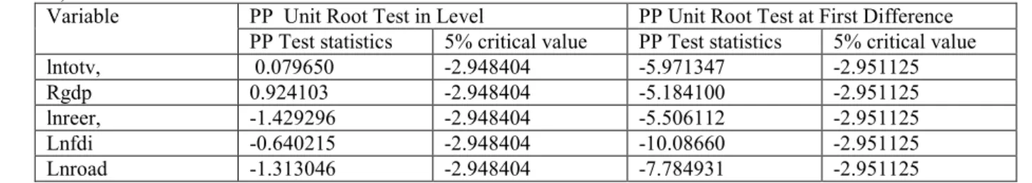
This test is done using the Augmented Dickey-Fuller (ADF) and Phillip Perron (PP) unit root tests. The ADF test is an extension of the Dickey-Fuller test because the regression has been augmented with the lagged changes. When the ADF and PP test statistics is larger than the critical value in absolute terms, the null hypothesis of unit root is rejected, and if the ADF and PP test statistics is less than the critical value in absolute terms, we fail to reject the null hypothesis. Table (3.1 a- and -b) shows the results of ADF and PP test for unit root. All variables are in logarithmic forms.

Table: 3.1 ADF and PP Unit Root Test a) ADF unit root test

Variable ADF Unit Root Test in Level ADF Unit Root Test at First Difference ADF Test statistics 5% critical value ADF Test statistics 5% critical value

lntotv, -0.250213 -2.948404 -4.729803 -2.954021

Rgdp 0.349382 -2.948404 -5.129080 -2.951125

lnreer, -1.408172 -2.948404 -5.521640 -2.951125

Lnfdi -0.318623 -2.954021 -7.785630 -2.954021

(5)

B) PP unit root test

Variable PP Unit Root Test in Level PP Unit Root Test at First Difference PP Test statistics 5% critical value PP Test statistics 5% critical value

lntotv, 0.079650 -2.948404 -5.971347 -2.951125

Rgdp 0.924103 -2.948404 -5.184100 -2.951125

lnreer, -1.429296 -2.948404 -5.506112 -2.951125

Lnfdi -0.640215 -2.948404 -10.08660 -2.951125

Lnroad -1.313046 -2.948404 -7.784931 -2.951125

In both case ADF and PP test at level the absolute values of the calculated test statistics for all variables are less than its critical value at 5 percent level of significance. The result indicates that all variables are non-stationary at level, i.e, the series appears to have unit root. So the null hypothesis that each variable has unit root cannot be rejected by both the ADF and PP test. However, after applying the first difference, we able to reject the null hypothesis since the data appear to be stationary at first difference. Therefore all variables are integrated of order one I (1)

3.2 Co-Integration Test Result

3.2.1 Optimal Lag Length Selection Criteria

In order to evaluate the VAR model the next step is to test for the existence of long-run relationship among the variables. Lack of co-integration between variables suggests the existence of no long-run relationship between them. Hence, the Johansen co-integration method is applied. However, before applying this test, it is necessary to determine the appropriate lag length. The determination of optimal lag length in the VAR system is a crucial issue since the co integration rank and resulting outputs are sensitive to the dynamic structure of the system. In this study, standard lag length selection criteria are used to select the number of lags of the VAR: the sequential modified likelihood ratio (LR) test, the Akaike information Criterion (AIC), the Final Prediction Error (FPE), the Hannan-Quinn Information Criterion (HQ), and the Schwarz Information Criterion (SIC) are criteria’s to select the optimal lag length. As presented in table (3.2) we can see that three of the criteria’s select lags two as the optimal lag length for the model. However, in order to make sure that lags with significant information content are not excluded from the VAR system of the model, Wald Lag- Exclusion Tests were performed. Wald tests (appendices B) show that two lags are jointly significant for all the equations in the VAR system. The VAR was, therefore, estimated with two lags.

Table 3.2 lag selection criteria

Lag LogL LR FPE AIC SC HQ

0 -88.23122 NA 0.000265 5.953407 6.406894 6.105992

1 60.35373 234.1338 1.53e-07 -1.536589 0.050615* -1.002543 2 102.5995 53.76730* 6.20e-08* -2.581786 0.139137 -1.666278* 3 130.2998 26.86091 7.63e-08 -2.745441* 1.109199 -1.448472 * indicates lag order selected by the criterion

3.2.2 The Johansen Co-integration Test Results

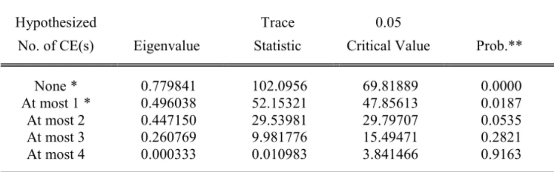
Since the included variables in model are I (1), the verification of the existence of a long run equilibrium relationship between the model variables is examined using Johansen cointegration approach. On the basis of the results of Trace test statistics in table (3.3), the Johansen procedure test result for co integration with two lags in the system indicates that there are two co integrating relationships. The trace test statistics fail to reject the null of at most two co integrating equations in the system.

(6)

Table: 3.3 Unrestricted Cointegration Rank Test (Trace)

Hypothesized Trace 0.05

No. of CE(s) Eigenvalue Statistic Critical Value Prob.**

None * 0.779841 102.0956 69.81889 0.0000

At most 1 * 0.496038 52.15321 47.85613 0.0187

At most 2 0.447150 29.53981 29.79707 0.0535

At most 3 0.260769 9.981776 15.49471 0.2821

At most 4 0.000333 0.010983 3.841466 0.9163

Trace test indicates 2 cointegrating eqn(s) at the 0.05 level * denotes rejection of the hypothesis at the 0.05 level **MacKinnon-Haug-Michelis (1999) p-values

Occasionally, the number of cointegrating relationships implied by trace test and maximum eigenvalue test are different (appendix C). Since the trace statistics is more robust than the maximum eigenvalue statistics in testing for co-integration, the existence of two cointegrating relationships is accepted (Luintel & Khan, 1999). 3.3 Diagnostic Tests

Diagnostics test are usually undertaken to detect model misspecification and as a guide for model improvement. These tests include serial correlation, heteroscedasticity and normality tests. The serial correlation test can be done using the Durbin-watson test or the lagrange multiplier (LM) test. It helps to identify the relationship that may exist between the current value of the regression residuals and lagged values. The study used the LM test to investigate serial correlation. The null-hypothesis of the LM test that the residuals are not serially correlated is accepted at 5% level of significance (appendix D).

The Jarque-Bera normality test is used to see whether the regression errors are normally distributed. The Jarque-Bera test failed to reject the null hypothesis of normal distribution of the residuals. So Jarque-Bera test for normality shows the regression errors are normally distributed (appendix D).

The hetreroscedasticity test helps to identify whether the variance of the errors in the model are constant or not. The null-hypothesis of the test is that the errors are homoscedastic and independent of the regressors and that there is no problem of misspecification. The null-hypothesis that the residuals are homoscedasticity is accepted at 5% significance level (appendix D).

The stability of the VAR model is tested by an inverse root of autoregressive characteristic polynomial. The result of the test is shown by a graphical representation on figure 3.1. It shows that the VAR model is stable as the entire modulus lie inside the circle showing that all the values are less than unity except the one.

Figure 3.1: Inverse Root of AR Characteristics Polynomial

-1.5 -1.0 -0.5 0.0 0.5 1.0 1.5 -1.5 -1.0 -0.5 0.0 0.5 1.0 1.5 Inverse Roots of AR Characteristic Polynomial

3.4 Vector Error Correction Model (VECM)

The presence of cointegration between variables in the cointegration test result suggests that the presences of a long term relationship among the variables. Then, a vector error correction model which is a restricted VAR

(7)

model that has cointegration restrictions built in to the specification. It is designed for use with nonstationary series that are known to be cointegrated. The vector error correction specification restricts the long-run behavior of the endogenous variables to converge to their cointegrating relationships while allowing a wide range of short-run dynamics. The cointegrating term (the error correction term) corrects the deviation from long-run equilibrium gradually through a series of partial short run adjustments (Eviews 9.1 User′s Guide II, 2015). So, the VEC model is convenient for the simultaneous analysis of long-run equilibrium relationships between variables as well as for their adjustment to deviations from this equilibrium in the short-run.

3.4.1 Long-Run Relationship in the export Model

As discussed in the co integration test result previously, the Johansen trace statistics indicated that the presence of two co integrating vectors/equations. However, the objective of this study is analyzing the relative impact real effective exchange rate on the performance of major export commodities. Therefore, the model estimated the unrestricted co integrating vector with ad-hoc normalization on LNTOTV. After normalization the first co integrating vector on LNTOTV normalized co integrating coefficients were estimated as below.

LFDI

LNREER

LNROAD

LNRGD

LNTOTV

=

10 .

31 −

2 .

00 +

2 .

20 +

1 .

23 +

0 .

25

[

6 .

12

]

[

−

5 .

54

]

[

−

3 .

11

]

[

−

3 .

32

]

R-squared =69.25 prob (F-statistic) = 0.032

Adj R-squared= 52.8

In the above estimated long-run model foreign direct investment and total engineered road have the expected sign as anticipated while real effective exchange rate and real gross domestic product have opposite sign from the anticipated.

The coefficient of foreign direct investment is positive as per the theoretical expectation in the long run. When we look at the degree of responsiveness, if FDI at time t increases by 1%, value of export responds to it increasing by 0.25 percent. Foreign direct investment (FDI) is statistically significant at 5 % significant level. A positive and significant relationship between export performance and FDI in Ethiopia indicates that the contribution of FDI to capital formation which helps to increase the performance exports in Ethiopia.. Thus, export performance positively responds to FDI in the long run.

The other important explanatory variable is kilometers of total engineered roads which is a proxy of infrastructural facilities. The above relation shows that an increase in the kilometers of engineered roads by 1% will increase the total value of exports of major export commodity by a magnitude of 2.20 percent. Infrastructural facility particularly, the expansion of roads is big determinant of country’s export performance. It plays an important role, especially at the early stages of export sector development. Most LDCs countries are characterized by poor transport infrastructure, which is a major impediment to trade, competitiveness and sustainable development and isolates countries, inhibiting their participation in global production networks. Due to poor internal transport infrastructure, LDCs transport costs are high making their exports expensive and uncompetitive and reducing foreign earnings from exports. So infrastructural development help to increase export performance of a country through increasing competitiveness by making their export cheap.

Real Effective Exchange Rate (REER) was found to be significant, but with unexpected positive sign. The unexpected positive relationship registered from the result of the estimated model might be due to different reasons. For instance, if real effective exchange rate increases, domestic currency will appreciate. The appreciation of domestic currency has obviously negative impact on exports since it decreases the competitiveness of the country’s export in the world market. On the hand, appreciation will also make imports cheap. Following the cheapness of import, domestic exporters may get incentive to import high quantities of different machineries, instruments, chemicals and others that will increase the productivity of goods and services in general and major export commodities in particular so devaluation leads to decrease in volume of export by increasing cost of inputs which further leads to decline in value of export.

Real GDP also revealed unexpected sign which is negative this negative relationship between GDP and value of export of major export commodity might be justified in such a way that when GDP of the country increases, domestic absorption will definitely increase. If domestic absorption increases, obviously export of major export products will decrease.

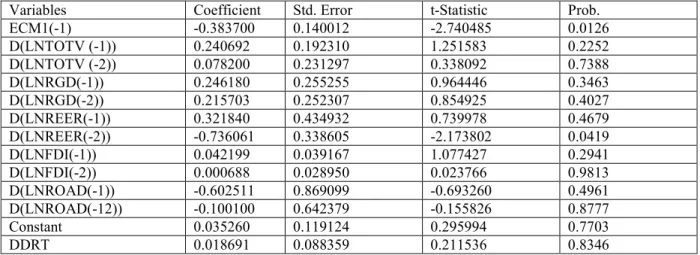
3.4.2 Short-Run Relationship in the export Model

Having already obtained the long-run model and estimated the coefficients, the next step was estimation of coefficients of the short-run dynamics that have important implications. Hence, an error correction model was estimated that incorporates the short term interactions and the speed of adjustment towards long run equilibrium.

(8)

Table 3.4 short run relationship

Variables Coefficient Std. Error t-Statistic Prob.

ECM1(-1) -0.383700 0.140012 -2.740485 0.0126 D(LNTOTV (-1)) 0.240692 0.192310 1.251583 0.2252 D(LNTOTV (-2)) 0.078200 0.231297 0.338092 0.7388 D(LNRGD(-1)) 0.246180 0.255255 0.964446 0.3463 D(LNRGD(-2)) 0.215703 0.252307 0.854925 0.4027 D(LNREER(-1)) 0.321840 0.434932 0.739978 0.4679 D(LNREER(-2)) -0.736061 0.338605 -2.173802 0.0419 D(LNFDI(-1)) 0.042199 0.039167 1.077427 0.2941 D(LNFDI(-2)) 0.000688 0.028950 0.023766 0.9813 D(LNROAD(-1)) -0.602511 0.869099 -0.693260 0.4961 D(LNROAD(-12)) -0.100100 0.642379 -0.155826 0.8777 Constant 0.035260 0.119124 0.295994 0.7703 DDRT 0.018691 0.088359 0.211536 0.8346

An error correction model (ECM) is built to capture the short run dynamics. The short run dynamics model provides information on how adjustments are taking place among the variables under study, in order to establish long run equilibrium in response to short run disturbances in the export performance of Ethiopia. As presented in table 3.4 the coefficient of the error correction term is with its negative expected sign and statistically significant, estimated at around – 0.3837. The size of the coefficient suggests that about 38.37 percent of the export disequilibria in Ethiopia will adjust towards the long run equilibrium in a given year.

The real effective exchange rate is negatively related to total value of export and is the only significant variable in the short-run. This implies that devaluation of the domestic currency in the short-run encourages exports. However, this contradicts the finding for the long-run relationship between the two variables. A two period lagged relationship between real effective exchange rate and growth in value of export shows that a change in the former variable has some impact on the production of some exportable items after a years. Most of the exports of Ethiopia are primary commodities produced by the agricultural sector. It is true that the production/supply of agriculture sector is not elastic in responding to changes in exchange rate as it takes some time to produce the commodities i.e. Production does not respond immediately to changes in real effective exchange rate. Thus, it may be logical to find a two period lagged relationship between real effective exchange rate and value of export growth in Ethiopia.

The insignificant positive coefficient of LNROAD in the short-run might be due to the time lag of the contribution of the infrastructure investment such as construction of road that has a long gestation period to give a return to increase export which shows the underdevelopment of the road sector in the short-run. But from the long-run point of view, LNROAD is highly significant indicating the importance of road growth for export of major export commodities.

3.5 Impulse Response

Impulse response function is used to trace the effect of a one standard deviation shock to one of the innovations on current and future values of the endogenous variables. We can identify the positive or negative impact of the variables and determine how long it would take for that effect to work. It is a method of assessing the interaction among the variables in the VAR.

Table (3.5) below shows that how total value of earning responds to a one standard deviation of the independent variables at any point in time. The result indicates that in response to one standard deviation shock of LNTOT, TOTV itself increases by 0.22 percent in the first year. It is also shown that in the first period a one standard deviation disturbance originating from the other variables do not have any impact on the total value of export. A two standard deviation disturbance originating from LNROAD produces a 0.012 in TOTV in the second period. Its effect continues to grow as the forecast period extend and reaches 0.075 at the 10th year. LNFDI binging from the second year although decline trend affect and grow to the long run reaching around 1.69 percent in the 10th period. The graphical depiction of impulse response is presented in appendices E

(9)

Table: 3.5 Impulse Response of TOTV

Period LNTOTV LNROAD LNRGDP LNREER LNFDI

1 0.222172 0.000000 0.000000 0.000000 0.000000 2 0.176647 0.012810 -0.007808 0.000593 0.108114 3 0.183814 0.040649 0.013356 0.005697 0.069806 4 0.130378 0.048268 0.006140 -0.022065 0.048893 5 0.132988 0.064323 -0.008227 -0.011443 0.028624 6 0.088608 0.070847 -0.021312 -0.007683 0.033492 7 0.072981 0.077078 -0.022872 0.004249 0.022091 8 0.046011 0.076385 -0.023688 0.006000 0.020297 9 0.041570 0.076746 -0.022052 0.012008 0.015258 10 0.032238 0.074932 -0.021072 0.012892 0.016955 3.6 Variance decomposition

Variance decomposition provides a different method of depicting the system dynamics. It decomposes variation in an endogenous variable in to the component shocks to the endogenous variables in the VAR. It gives information about the relative importance of each random change in the explanatory variables in the VAR Table 3.6 shows that the variation in the growth total value of export is explained only by its lagged value in the first period. After the first period, the variation in total value of export growth can be explained by a group of other endogenous variables in the system. In the table below, the variance estimates indicate that a greater proportion of the variation in total value of export is due to its own innovations. The variation due to the other variables is smaller. The other four variables together explain approximately 27.32% of the future variation in TOTV growth in Ethiopia. The remaining 72.68% are due to changes in total value of export itself within the period under consideration. Graphical representation of variance decomposition is presented in appendices E Table 3.6 Variance Decomposition

Period S.E. LNTOTV LNROAD LNRGDP LNREER LNFDI

1 0.222172 100.0000 0.000000 0.000000 0.000000 0.000000 2 0.304103 87.11693 0.177437 0.065918 0.000380 12.63934 3 0.364694 85.97757 1.365704 0.179959 0.024667 12.45210 4 0.394012 84.60823 2.670751 0.178457 0.334740 12.20782 5 0.422003 83.68749 4.651464 0.193574 0.365333 11.10214 6 0.438853 81.46104 6.907287 0.414827 0.368466 10.84838 7 0.452646 79.17172 9.392368 0.645245 0.355163 10.43551 8 0.462438 76.84419 11.72722 0.880603 0.357113 10.19087 9 0.471519 74.69006 13.92904 1.065728 0.408340 9.906831 10 0.479460 72.68856 15.91390 1.223877 0.467227 9.706433 4 Conclusion and Recommendation

4.1 Conclusions

Ethiopia has for long been dependent on primary commodities to partially meet its foreign exchange earnings. However, foreign exchange earnings attained from these traditional products which are mainly agricultural commodities could not match with the highly increasing demand as a result governments of Ethiopia works to improve its trade performance through different policies like exchange rate policies. That is why this study has made an attempt to examine the effect of currency devaluation on major export commodities in Ethiopia which are mainly traditional agricultural commodities. In other words, the central question investigated in this study is whether or not currency devaluation significantly affects the performance of major export commodities in Ethiopia. To address this question, time serious data ranging from the year 1980/81 up to 2015/16 was utilized. The study used secondary data collected from different sources. In this study values of major export commodity was used as dependent variable and variables like real effective exchange rate, total engineered road, real gross

(10)

of export in Ethiopia and may stay to play its major role in the future because having an improved road infrastructure assist to increase in performance of trade in the following ways first , road transport provide a physical access to resource and market, second reduces the price of domestic product and promote competitiveness in local and international market third expansion of road network contribute to economic diversification and enable exploitation of economies of scale which help to increase export and reduce vulnerability of shocks in trade .

The study also found impact of real effective exchange rate on performance of export of major export commodities works through the aggregate demand channel in the short-run and the aggregate supply channel in the long-run i.e. decrease/devaluation in the value of the domestic currency increase volume of export only in the short run. In the long-run, devaluation leads to decrease in export. It may be the case that in the short run primary exports can be promoted through devaluation of the currency and this does not much affect the economy through the import sector as the economy does not much depend on foreign capital for investment.

Different reasons are given for the negative impact of devaluation on export in the long-run. First developing countries economy depends on foreign capital for investment and the demand for their export elasticity is low. Devaluation increases the cost of importing this capital there by reduces productivity of exportable commodities. The other argument is in terms of increase in the cost of imported raw materials due to depreciation. The major imported items in Ethiopia are petroleum products which absorbs more than half of its foreign earnings. As the country devaluates its currency, it means that the price of oil increases. In this case, the government cannot allocate more of its foreign earnings to development investments. It also increases the cost of production and this cause inflation which leads to decrease in productivity. In both cases, the results would be decline in volume of export which in turn leads to decline in the value of export.

The findings of the study also reveal that foreign direct investment and gross domestic product significantly affect export earning of Ethiopia in the long run. Foreign direct investment inflow is vital for employment creation, capital formation and for transfer of knowledge and technology which helps in improvement for infrastructure facility and increase export performance of Ethiopia.

4.2 Recommendation

Based on the findings of the study the following policy recommendations are forwarded to improve the export performance of Ethiopia.

First the findings of the study shows that even though the government’s policy makers should have to give a due emphasis for all factors either price and non-price factors that significantly affected the traditional export commodity performance of country, emphasis should be given for especially non-price factors such as the provision of infrastructure like roads facilities which have to take the lions share. For instance, if we look at the results of Impulse response and variance decompositions indicate the permanent effect of road on the total value earning is high and in the estimated long run model the coefficient of kilometers of total road is larger than other variables. This implies that road network is a major factor affecting the sector and its improvement is crucial for the promotion of major export commodities in Ethiopia.

Second Real effective exchange rate and performance of export are negatively related in the short-run i.e. decrease/devaluation in real effective exchange rate increases export in short run. Therefore, a smooth and periodical devaluation of the “birr” may be helpful to boost export in the short run because devaluation of the domestic currency encourages foreign demand for exports as the price of the exportable items become cheaper in foreign currency for foreigners. Increase in foreign demand for exports encourages domestic producers of the same items. The results of these would be increase the volume of export. But in the long run result shows that there is a positive relationship between real effective exchange rate and value of export. So although it has been recommended that the real effective exchange rate should be kept low (devaluate) in the short run it does not mean that it shall remain low all the time. The long-run result shows that after a periodical devaluation of the “birr” for some time, it may be helpful to change the policy as the direction of the relationship changes and it shows devaluating of currency should not be used as long lasting policy.

The last but not least implication is that government should encourage the flow of foreign direct investment in the country as it is an important factor in influencing the export performance in the long run. With regard to the magnitude of the effect, the result suggests that an increase by 1% of FDI can be expected to result in improving export performance by 0.25 percent. In general concerned body should works to strengthen and extend infrastructure since it helps to increase the performance of export because if for example total road network, improved it would enable producers to sell their product in the nearby markets in short period of time. This will in turn make them to shift from subsistence production to commercial production. This will lead to again a higher proportion of gross domestic product constituting export volumes.

Reference

(11)

Befikadu, D. and Kibere, M. (1994). Post devaluation of the Ethiopian economy. From stagnation to stagflation, in Mekonene Tadesse and Abdulahamid Bedri Kello the Ethiopian economy problem of adjustment,. proceeding of the second annual conerence on ethiopian economy.

Elbadawi, I. (2014). Can Africa export manufactures the role of Endowment, Exchange Rates and and transaction costs, world bank, . policy research work paper.

Elias Ali,. (2011). The effect of depreciation of birr on major export product s of ethiopia: the case of hides and skins. Addis Abeba University Ethiopia.

EViews 9.1 User′s Guide II. (2015). Quantitative Micro Software, IHS Global Inc., USA.

Eyayu, T. (2011). Determents of Agricultural Export in the Sub-Saharan Africa food and Agricultural organization. a Review report (2007) global Hides and Skins markets; A Review short term outlook, FAO. Geberelibanos, H. (2005). The effect of exchange rate policy on agricultural export Commodities in Ethiopia the

cause of oilseeds. Msc. thesis, Addis Ababa University Addis Ababa Ethiopia.

Ghatak, S. (1995). Monetary economics in developing countries . 2nd edition, Macmillan press ltd, UK.

Kumar, J. (1998). Technology , market structure and internationalization. issue and policies for developing countries, Routledge, New York.

Luintel, K.B. and Khan M,. (1999). Quantitative reassessment of the Finance and Growth Nexus. evidence from a multivariate VAR Journal of Development Economics.

Mekbib, N. (2008). The per- shipment loan utilization in exporting agricultural product in Ethiopia. A project paper submitted in partial fulfillment of the requirements for the degree of Master of Science in according and finance.

Mouz, M . (2005). determinates of agricultural export in Ethiopia.

Moya, M. and Watundu, S. (2009). Econometric Analysis of Real Effective Exchange Rate On Gross Domestic product of Uganda. E-Journal of Business And Economic Issues, Volume Iv Issue II.

Nouria, R. ,plane, P. and Sekkat, K. (2010). Exchange rate undervaluation to foster manufactured exports, deliberate strategies. working paper no.1148.

Raddatz.(2008). Exchange rate volatility and trade in South Africa. the World Bank Development Research group macroeconomics and growth team, Washington, Dc.

Thapa, N.B. (2002). An Econometric Analysis of the Impact of Real Effective Exchange Rate on Economic Activities in Nepal. Research Department, Nepal Rastra Bank.

Appendices

A) Unit root test

Null Hypothesis: LNTOTV has a unit root Exogenous: Constant

Lag Length: 0 (Automatic - based on SIC, maxlag=9)

t-Statistic Prob.*

Augmented Dickey-Fuller test statistic -0.250213 0.9224

Test critical values: 1% level -3.632900

5% level -2.948404

10% level -2.612874

*MacKinnon (1996) one-sided p-values. Null Hypothesis: D(LNTOTV) has a unit root Exogenous: Constant

t-Statistic Prob.*

Augmented Dickey-Fuller test statistic -4.729803 0.0006

Test critical values: 1% level -3.646342

5% level -2.954021

(12)

Null Hypothesis: LNROAD has a unit root Exogenous: Constant

t-Statistic Prob.* Augmented Dickey-Fuller test statistic -1.346349 0.5969 Test critical values: 1% level -3.632900

5% level -2.948404

10% level -2.612874

*MacKinnon (1996) one-sided p-values. Null Hypothesis: D(LNROAD) has a unit root Exogenous: Constant

5% level -2.951125

10% level -2.614300

*MacKinnon (1996) one-sided p-values.

Null Hypothesis: LNRGDP has a unit root Exogenous: Constant

t-Statistic Prob.* Augmented Dickey-Fuller test statistic 0.349382 0.9777 Test critical values: 1% level -3.632900

5% level -2.948404

10% level -2.612874

*MacKinnon (1996) one-sided p-values. Null Hypothesis: D(LNRGDP) has a unit root Exogenous: Constant

5% level -2.951125

10% level -2.614300

(13)

Null Hypothesis: LNREER has a unit root Exogenous: Constant

5% level -2.948404

10% level -2.612874

*MacKinnon (1996) one-sided p-values. Null Hypothesis: D(LNREER) has a unit root Exogenous: Constant

5% level -2.951125

10% level -2.614300

*MacKinnon (1996) one-sided p-values. Null Hypothesis: LNFDI has a unit root Exogenous: Constant

5% level -2.954021

10% level -2.615817

*MacKinnon (1996) one-sided p-values. Null Hypothesis: D(LNFDI) has a unit root Exogenous: Constant

5% level -2.954021

10% level -2.615817

(14)

B) Lag Exclusion Wald Test VAR Lag Exclusion Wald Tests Included observations: 34

Chi-squared test statistics for lag exclusion: Numbers in [ ] are p-values

LNTOTV LNROAD LNRGDP LNREER LNFDI Joint

Lag 1 26.32401 39.50162 20.90489 70.33193 11.26278 239.6155 [ 7.72e-05] [ 1.88e-07] [ 0.000844] [ 8.74e-14] [ 0.046412] [ 0.000000] Lag 2 5.332638 5.628946 4.019968 28.22053 5.719476 57.34297

[ 0.376647] [ 0.344014] [ 0.546545] [ 3.30e-05] [ 0.334479] [ 0.000240]

df 5 5 5 5 5 25

C) Johanson cointegration test

Series: LNTOTV LNROAD LNRGDP LNREER LNFDI Exogenous series: DUMMY_DROU

Warning: Critical values assume no exogenous series Lags interval (in first differences): 1 to 2

Unrestricted Cointegration Rank Test (Trace)

Hypothesized Trace 0.05

No. of CE(s) Eigenvalue Statistic Critical Value Prob.** None * 0.779841 102.0956 69.81889 0.0000 At most 1 * 0.496038 52.15321 47.85613 0.0187 At most 2 0.447150 29.53981 29.79707 0.0535 At most 3 0.260769 9.981776 15.49471 0.2821 At most 4 0.000333 0.010983 3.841466 0.9163 Trace test indicates 2 cointegrating eqn(s) at the 0.05 level

* denotes rejection of the hypothesis at the 0.05 level **MacKinnon-Haug-Michelis (1999) p-values

Unrestricted Cointegration Rank Test (Maximum Eigenvalue)

Hypothesized Max-Eigen 0.05

No. of CE(s) Eigenvalue Statistic Critical Value Prob.** None * 0.779841 49.94241 33.87687 0.0003 At most 1 0.496038 22.61340 27.58434 0.1906 At most 2 0.447150 19.55804 21.13162 0.0818 At most 3 0.260769 9.970793 14.26460 0.2139 At most 4 0.000333 0.010983 3.841466 0.9163 Max-eigenvalue test indicates 1 cointegrating eqn(s) at the 0.05 level * denotes rejection of the hypothesis at the 0.05 level

(15)

D) Diagnostics test

1) Breusch-Godfrey Serial Correlation LM Test:

F-statistic 0.556693 Prob. F(2,18) 0.5827

Obs*R-squared 1.922304 Prob. Chi-Square(2) 0.3825 Ho: No serial correlation

H1: Serial correlation

Therefore, we fail to reject the null hypothesis.

2) Heteroskedasticity Test: Breusch-Pagan-Godfrey

F-statistic 1.684275 Prob. F(16,16) 0.1537 Obs*R-squared 20.70618 Prob. Chi-Square(16) 0.1901 Scaled explained SS 6.513024 Prob. Chi-Square(16) 0.9815 Ho: Homoskedasticity

H1: Heteroskedasticity

Thus, we accept the null hypothesis of constant variance or homoskedastic 3) Jarque-Bera Normality Test

0 1 2 3 4 5 6 7 8 -0.4 -0.3 -0.2 -0.1 0.0 0.1 0.2 0.3 Series: Residuals Sample 1983 2015 Observations 33 Mean 2.14e-15 Median 0.006610 Maximum 0.325822 Minimum -0.378233 Std. Dev. 0.167536 Skewness -0.075589 Kurtosis 2.712698 Jarque-Bera 0.144921 Probability 0.930102

Since the probability of Jacque-Bera is equal to 0.93 which is greater than 0.05, the distribution is normal distribution.

(16)

E) Impulse response of TOTV -.1 .0 .1 .2 .3 1 2 3 4 5 6 7 8 9 10

Response of LNTOTV to LNTOTV

-.1 .0 .1 .2 .3 1 2 3 4 5 6 7 8 9 10

Response of LNTOTV to LNROAD

-.1 .0 .1 .2 .3 1 2 3 4 5 6 7 8 9 10 Response of LNTOTV to LNRGDP -.1 .0 .1 .2 .3 1 2 3 4 5 6 7 8 9 10

Response of LNTOTV to LNREER

-.10 -.05 .00 .05 .10 .15 .20 .25 .30 1 2 3 4 5 6 7 8 9 10

(17)

F) Variance decomposition 0 20 40 60 80 100 1 2 3 4 5 6 7 8 9 10

Percent LNTOTV variance due to LNTOTV

0 20 40 60 80 100 1 2 3 4 5 6 7 8 9 10

Percent LNTOTV variance due to LNROAD

0 20 40 60 80 100 1 2 3 4 5 6 7 8 9 10

Percent LNTOTV variance due to LNRGDP

0 20 40 60 80 100 1 2 3 4 5 6 7 8 9 10

Percent LNTOTV variance due to LNREER

0 20 40 60 80 100 1 2 3 4 5 6 7 8 9 10