Optimization design of structures subjected to transient loads using first and second derivatives of dynamic displacement and stress

IOS Press

Optimization design of structures subjected to

transient loads using

first and second

derivatives of dynamic displacement and

stress

Qimao Liu

_{, Jing Zhang}

_{and Liubin Yan}

a_{Department of Civil and Structural Engineering, Aalto University, Espoo, Finland} b_{College of Civil and Architecture Engineering, Guangxi University, Nanning, China}

c_{Department of Mechanical Engineering, Indiana University-Purdue University Indianapolis, Indianapolis, IN,} USA

Received 16 September 2010 Revised 19 July 2011

Abstract.This paper developed an effective optimization method, i.e., gradient-Hessian matrix-based method or second order method, of frame structures subjected to the transient loads. An algorithm offirst and second derivatives of dynamic displacement and stress with respect to design variables is formulated based on the Newmark method. The inequality time-dependent constraint problem is converted into a sequence of appropriately formed time-independent unconstrained problems using the integral interior point penalty function method. The gradient and Hessian matrixes of the integral interior point penalty functions are also computed. Then the Marquardt’s method is employed to solve unconstrained problems. The numerical results show that the optimal design method proposed in this paper can obtain the local optimum design of frame structures and sometimes is more efficient than the augmented Lagrange multiplier method.

Keywords: Dynamic response optimization, gradient, Hessian matrix, time-dependent constraint

1. Introduction

Dynamic response analysis of structures subjected to transient loads often requires much more demanding

com-putational cost than static analysis. Therefore the efficiency of the optimization method becomes critical to

dy-namic response optimization problems. Mathematically, there are three types of dydy-namic response optimization

methods: zero order methods (nongradient-based algorithms),first order methods (gradient-based algorithms) and

second order methods (gradient-Hessian matrix-based algorithms). Generally, the first order methods are more

efficient than the zero order methods, and the second order methods are more efficient than thefirst order methods.

Zero order methods require only the information of dynamic responses to construct optimal algorithms. A lot of nongradient-based algorithms [1–4] have been developed to solve the optimization problem of structures subjected

to transient loads. First order methods require the information of dynamic responses and theirfirst derivatives with

respect to design variables to construct optimal algorithms. Therefore, it is very crucial to calculate efficiently the

∗_{Corresponding author: Qimao Liu, Department of Civil and Structural Engineering, Aalto University, Espoo, FI-00076 Aalto, Finland. Tel.:}

+358 9 470 23701; Fax: +358 9 470 23758; E-mail: [email protected]. ISSN 1070-9622/12/$27.502012 – IOS Press and the authors. All rights reserved

first derivatives of structural dynamic responses for gradient-based algorithms. However, many algorithms have been

developed to calculate dynamic responsefirst derivatives with respect to design variables (also called sensitivity

anal-ysis [5–12]). Today, the gradient-based algorithms are the mainstream pattern [13] to solve the optimization problem of structures subjected to transient loads. Much research [14–17] has been done to solve the structural dynamic response optimization problem with the gradient-based algorithms. Second order methods require the information of

dynamic responses, theirfirst and second derivatives with respect to design variables to construct optimal algorithms.

The Newton’s method and Quasi Newton’s method are the commonly used second order method. Although many

researchers have calculated dynamic responsefirst derivatives with respect to design variables, there is little literature

published on dynamic response second derivative analysis (also called Hessian matrix analysis). Second derivative

analysis is more complicated thanfirst derivative analysis. However, the efficiency of the optimization using second

derivative can be greatly improved when the gradient and Hessian matrix can be calculated efficiently. In this paper,

a gradient-Hessian matrix-based algorithm for optimization problem of structures subjected to transient loads is developed based on gradient and Hessian matrix calculations.

The purpose of this paper is to develop a gradient-Hessian matrix-based optimization method for structures subjected to dynamic loads. The main work of this paper is as follows: First, we formulate an algorithm to calculate

dynamic responses and theirfirst and second derivatives with respect to design variables. The algorithm is achieved

by direct differentiation and only a single dynamics analysis, based on Newmark-βmethod [18], is required. Second,

we formulate the time-dependent structural optimization model. In this model, total mass of the structure is the objective function. The dynamic responses including stresses of the beam element and nodal displacements are constraints. Third, the time-dependent optimization model is converted into a sequence of appropriately formed unconstrained integral mathematic models using the interior penalty function method. The gradient and Hessian

matrixes of the interior penalty functions are also calculated using thefirst and second derivatives of dynamic

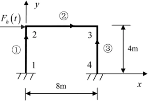
responses. Fourth, Marquardt’s method [19], a gradient-Hessian matrix-based algorithm, is employed to solve the unconstrained integral mathematic model. Finally, as the illustration of the developed approach, optimization designs of a plane frame subjected to the horizontal dynamic loads are demonstrated.

2. Calculation offirst and second derivatives

This section presents two subjects. Section 2.1 introduces the calculations offirst and second derivatives of

dynamic responses (i.e., nodal displacement and normal stress) with respect to design variables of structures.

Section 2.2 discusses how to calculatefirst and second derivatives of structural mass with respect to structural design

variables.

2.1. Calculation offirst and second derivatives of dynamic displacement and stress

Thefirst and second derivatives of dynamic response of structures are the prerequisites of an efficient

gradient-Hessian matrix-based algorithm. We will show here that, in a single structural dynamic analysis, thefirst and second

derivatives of a dynamic response can be derived simultaneously.

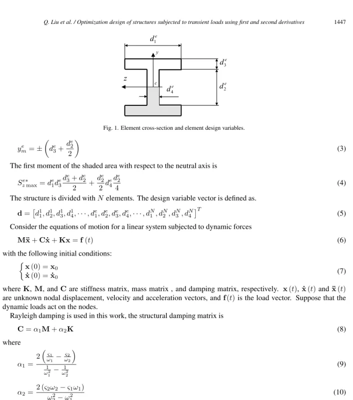
Plane beam element is used extensively in engineering. Therefore, the dynamic optimal design method is demon-strated with the plane beam element in this work. The element cross-section shown in Fig. 1 is H structural-steel

shape. The design variables of elementearede

1,de2,de3andde4. Pointcis the centroid of the element cross-section.

Axesyandzare the principal centroidal axes.

The cross-sectional area is

Ae= 2de₁d₃e+de₂de₄ (1)

The cross-sectional moment of inertia is

I_ze=d e 4de23 12 + 2 de 1de33 12 + de 3+d2e 2 ₂ de₁de₃ (2)

Fig. 1. Element cross-section and element design variables. y_me =± de₃+d e 2 2 (3)

Thefirst moment of the shaded area with respect to the neutral axis is

S_ze∗_max=de₁de₃d e 3+de2 2 + de 2 2 de4 de 2 4 (4)

The structure is divided withNelements. The design variable vector is defined as.

d=d1₁, d1₂, d1₃, d1₄,· · ·, de₁, d₂e, de₃, de₄,· · ·, d₁N, dN₂, dN₃, dN₄T (5)

Consider the equations of motion for a linear system subjected to dynamic forces

M¨x+C ˙x+Kx=f(t) (6)

with the following initial conditions:

x(0) =x0

˙x(0) = ˙x0 (7)

whereK,M, andCare stiffness matrix, mass matrix , and damping matrix, respectively. x(t), _˙x(t)and_¨x(t)

are unknown nodal displacement, velocity and acceleration vectors, andf(t)is the load vector. Suppose that the

dynamic loads act on the nodes.

Rayleigh damping is used in this work, the structural damping matrix is

C=α_1M+α_2K (8) where α₁= 2 ς1 ω1 −ω2ς2 1 ω2₁ −ω1₂2 (9) α₂= 2 (ς2ω2−ς1ω1) ω₂2−ω₁2 (10)

whereω₁andω₂are thefirst and second natural frequency of the structure, respectively.ς₁andς₂are the damping

ratio. In this work,ς₁=ς₂= 0.02.α₁andα₂are constants.

Equations (6) and (7) must be satisfied for all time periodt ∈ [0,Γ]. Γ is the duration of the dynamic loads.

In practice, the solution of this initial-boundary-value problem (IBVP) requires integration through time. This is achieved numerically by discretising in time the continuous temporal derivatives that appear in the equation. Any one of the time integration procedures can be used for this purpose. The most widely used family of direct time integration methods for solving Eq. (6) is the Newmark family of methods. The Newmark method can be formulated

by considering equilibrium at any discrete timet+ Δt, and is given by the following equation:

The nodal displacements, nodal accelerations and nodal velocities can be achieved at any timet+ Δtby solving

Eq. (11).

Perhaps the most widely used direct method for the equation of motion (6) is the Newmark method, an

im-plicit technique, which consists of the followingfinite difference assumptions with regard to the evolution of the

approximate solution: x(t+ Δt) =_x(t) + Δt_˙x(t) + Δt2 1 2−β ¨ x(t) +β_¨x(t+ Δt) (12) ˙x(t+ Δt) =_˙x(t) + Δt[(1−δ)_¨x(t) +δ_¨x(t+ Δt)] (13)

where any particular choice of the parametersβ andδdetermines the stability and accuracy characteristics of the

solution. In this work, parametersδ0.5 andβ = 0.25 (0.5 +δ)2. We define the integral constants:a₀ = 1

βΔt2,

a₁=_βδ_Δt,a₂=_βΔ1_t,a₃=₂1_β−1,a₄= δ_β−1,a₅= Δ₂t _βδ −2

,a₆= Δt(1−δ),a₇=δΔt. The parametersβ

andδwill be replaced by those constants in the following formulas.

In addition to Eqs (12) and (13) the equilibrium Eq. (11) at time stationt+ Δtis considered. This way a system of

equations is formed for the determination of the three unknowns_x(t+ Δt), _˙x(t+ Δt)and_x¨(t+ Δt), assuming

that the displacement, velocity, and acceleration vectors at the previous time stationthave already been computed.

Thus, the solution for the displacement vector is

K∗x(t+ Δt) =_F∗(t+ Δt) (14)

where

K∗=K+a_0M+a_1C (15)

and

F∗(t+ Δt) =_f(t+ Δt) +_M[a_0x(t) +a_2˙x(t) +a_3¨x(t)] +_C[a_1x(t) +a_4˙x(t) +a_5¨x(t)] (16)

The accelerations,x¨(t+ Δt), which are required for the computations at the next time station, can be computed

as ¨

x(t+ Δt) =a₀[x(t+ Δt)−_x(t)]−a_2˙x(t)−a_3¨x(t) (17)

while the velocities,˙x(t+ Δt), can be obtained directly from equation (13), as follows.

˙x(t+ Δt) =_˙x(t) +a_6x¨(t) +a_7¨x(t+ Δt) (18)

When the dynamic loads act on the nodes, we only need to determine the internal forces and internal couples at

the center and two ends of the element. The element nodal force vector,_F¯e_{(t+ Δt), is}

¯

Fe(t+ Δt) =_K¯e_Teδe(t+ Δt) (19)

where_K¯e_{is the element stiffness matrix in a local coordinate system,T}e_{is the element coordinate transformation}

matrix,δe(t+ Δt)is the element nodal displacement vector in a local coordinate system.

The internal force vector at the center of element,_F¯e

M(t+ Δt), is ¯ FeM(t+ Δt) = −_F¯e 1(t+ Δt) −F¯2e(t+ Δt) le2F¯2e(t+ Δt)−F¯e3(t+ Δt) T (20)

where l_e is the length of element. The three terms, i.e., −_F¯e

1(t+ Δt), −F¯e2(t+ Δt) and le2F¯e2(t+ Δt)−

¯

Fe3(t+ Δt), are axial force, shear force and bending moment, respectively. F¯e1(t+ Δt), F¯e2(t+ Δt) and

¯

Fe3(t+ Δt)are thefirst, second and third term of the element nodal force vector,F¯e(t+ Δt), respectively.

The maximum stress at the center and two ends, i.e. theiend and thej end, of the element are calculated as

follows.

The maximum normal stress at theiend of the element is

σ_ixe (t+ Δt) =F¯ e 1(t+ Δt) Ae + ¯ Fe 3(t+ Δt)yme EIe z (21)

The maximum normal stress at thejend of the element is σ_jxe (t+ Δt) = F¯ e 4(t+ Δt) Ae + ¯ Fe 6(t+ Δt)yem EIe z (22) where_F¯e

4(t+ Δt)andF¯e6(t+ Δt)are the fourth and sixth term of the element nodal force vector,F¯e(t+ Δt),

respectively.

The maximum normal stress at the center of the element is

σ_Mxe (t+ Δt) = F¯ e M1(t+ Δt) Ae + ¯ FeM3(t+ Δt)yem EIe z (23) where_F¯e

M1(t+ Δt)andF¯eM3(t+ Δt)are the first and third term of the internal force vector at the center of

element,_F¯e

M(t+ Δt), respectively.

The maximum shear stress at theiend of the element is

τ_ixye (t+ Δt) = F¯ e 2(t+ Δt)Se∗zmax de₄Ie z (24)

The maximum shear stress at thejend of the element is

τ_jxye (t+ Δt) = F¯ e 5(t+ Δt)Sze∗max de 4Ize (25) where_F¯e

5(t+ Δt)is thefifth term of the element nodal force vector,F¯e(t+ Δt).

The maximum shear stress at the center of the element is

τ_Mxye (t+ Δt) = F¯ e M2(t+ Δt)Sze∗max de 4Ize (26) where_F¯e

M2(t+ Δt)is the second term of the internal force vector at the center of element,F¯eM(t+ Δt).

2.1.1. Formulas forfirst derivatives of dynamic displacement and stress

Now we will derive the formulas for thefirst derivatives of dynamic response, i.e., dynamic displacement and

stress. Differentiating Eq. (14) with respect to the design variabled_i, we have

K∗∂x(t_∂d+ Δt) i = ∂_F∗(t+ Δt) ∂d_i − ∂_K∗ ∂d_i x(t+ Δt) (27) where ∂_K∗ ∂d_i = ∂_K ∂d_i +a0 ∂_M ∂d_i +a1 ∂_C ∂d_i (28) and ∂_F∗(t+ Δt) ∂d_i = ∂_M ∂d_i [a0x(t) +a2˙x(t) +a3x¨(t)] +M a₀∂x(t) ∂d_i +a2 ∂_˙x(t) ∂d_i +a3 ∂_¨x(t) ∂d_i +∂C ∂d_i[a1x(t) +a4˙x(t) +a5¨x(t)] +C a₁∂x(t) ∂d_i +a4 ∂_˙x(t) ∂d_i +a5 ∂_x¨(t) ∂d_i (29)

After thefirst derivatives of displacement vector at timet+ Δtis obtained from Eq. (27), through differentiating

Eq. (17) with respect to design variablesd_i, we have

∂_¨x(t+ Δt) ∂d_i =a0 ∂_x(t+ Δt) ∂d_i − ∂_x(t) ∂d_i −a₂∂˙x(t) ∂d_i −a3 ∂_¨x(t) ∂d_i (30)

Then, thefirst derivatives of acceleration vector at timet+ Δtis obtained from Eq. (30). Differentiating Eq. (18)

with respect to design variabled_i, we have

∂_˙x(t+ Δt) ∂d_i = ∂_˙x(t) ∂d_i +a6 ∂_¨x(t) ∂d_i +a7 ∂_¨x(t+ Δt) ∂d_i (31)

Differentiating Eq. (19) with respect to the design variabled_i, we have ∂_F¯e_{(t+ Δt)} ∂d_i = ∂_K¯e ∂d_i T e_δe_{(t+ Δt) +K¯}e_Te∂δe(t+ Δt) ∂d_i (32) where∂δe(t+Δt)

∂di can be calculated from

∂x(t+Δt)

∂di .

Differentiating Eq. (20) with respect to the design variabled_i, we have

∂_F¯e M(t+ Δt) ∂d_i = −∂F¯e1(t+Δt) ∂di − ∂F¯e2(t+Δt) ∂di le 2∂ ¯ Fe 2(t+Δt) ∂di − ∂F¯e3(t+Δt) ∂di T (33)

Differentiating Eq. (21) with respect to the design variabled_i, we have

∂σe ix(t+ Δt) ∂d_i = ∂_F¯e 1(t+ Δt) ∂d_i 1 Ae− ¯ Fe 1(t+ Δt) Ae2 ∂Ae ∂d_i +∂F¯e3(t+ Δt) ∂d_i ye_m EIe z +F¯e3(t+ Δt) EIe z ∂ye_m ∂d_i − ¯ Fe3(t+ Δt)yem EIe2 z ∂I_ze ∂d_i (34)

Differentiating Eq. (22) with respect to the design variabled_i, we have

∂σe_jx(t+ Δt) ∂d_i = ∂_F¯e 4(t+ Δt) ∂d_i 1 Ae− ¯ Fe 4(t+ Δt) Ae2 ∂Ae ∂d_i +∂F¯e6(t+ Δt) ∂d_i ye m EIe z +F¯e6(t+ Δt) EIe z ∂ye m ∂d_i − ¯ Fe 6(t+ Δt)yem EIe2 z ∂Ie z ∂d_i (35)

Differentiating Eq. (23) with respect to the design variabled_i, we have

∂σe Mx(t+ Δt) ∂d_i = ∂_F¯e M1(t+ Δt) ∂d_i 1 Ae − ¯ Fe M1(t+ Δt) Ae2 ∂Ae ∂d_i +∂F¯eM3(t+ Δt) ∂d_i ye m EIe z +F¯eM3(t+ Δt) EIe z ∂ye m ∂d_i − ¯ Fe M3(t+ Δt)yme EIe2 z ∂Ie z ∂d_i (36)

Differentiating Eq. (24) with respect to the design variabled_i, we have

∂τe ixy(t+ Δt) ∂d_i = ∂_F¯e₂(t+ Δt) ∂d_i S_ze∗_max de 4Ize +∂Sze∗max ∂d_i ¯ Fe2(t+ Δt) de 4Ize −∂de4 ∂d_i ¯ Fe 2(t+ Δt)Sze∗max de2 4 Ize −∂Ize ∂d_i ¯ Fe 2(t+ Δt)Sze∗max de 4Ize2 (37)

Differentiating Eq. (25) with respect to the design variabled_i, we have

∂τe jxy(t+ Δt) ∂d_i = ∂_F¯e 5(t+ Δt) ∂d_i S_ze∗_max de 4Ize +∂Sze∗max ∂d_i ¯ Fe 5(t+ Δt) de 4Ize −∂de4 ∂d_i ¯ Fe 5(t+ Δt)Sze∗max de2 4 Ize −∂Ize ∂d_i ¯ Fe 5(t+ Δt)Sze∗max de 4Ize2 (38)

Differentiating Eq. (26) with respect to the design variabled_i, we have

∂τ_Mxye (t+ Δt) ∂d_i = ∂_F¯e_M2(t+ Δt) ∂d_i S_ze∗_max de 4Ize +∂Sze∗max ∂d_i ¯ FeM2(t+ Δt) de 4Ize −∂de4 ∂d_i ¯ Fe M2(t+ Δt)Sze∗max de2 4 Ize −∂Ize ∂d_i ¯ Fe M2(t+ Δt)Sze∗max de 4Ize2 (39)

2.1.2. Formulas for second derivatives of dynamic displacement and stress

Now we will derive the formulas for the second derivatives of dynamic response, i.e., dynamic displacement and

stress. Further differentiating Eq. (27) with respect to the design variabled_j, we have

K∗∂ 2_{x(t+ Δt)} ∂d_i∂d_j = ∂2_F∗(t+ Δt) ∂d_i∂d_j − ∂2_K∗ ∂d_i∂d_jx(t+ Δt)− ∂_K∗ ∂d_i ∂_x(t+ Δt) ∂d_j − ∂_K∗ ∂d_j ∂_x(t+ Δt) ∂d_i (40) where ∂2_K∗ ∂d_i∂d_j = ∂2_K ∂d_i∂d_j +a0 ∂2_M ∂d_i∂d_j +a1 ∂2_C ∂d_i∂d_j (41) and ∂2_F∗(t+ Δt) ∂d_i∂d_j = ∂2_M ∂d_i∂d_j [a0x(t) +a2˙x(t) +a3¨x(t)] + ∂_M ∂d_i a₀∂x(t) ∂d_j +a2 ∂_˙x(t) ∂d_j +a3 ∂_¨x(t) ∂d_j +∂M ∂d_j a₀∂x(t) ∂d_i +a2 ∂_˙x(t) ∂d_i +a3 ∂_¨x(t) ∂d_i +M a₀∂ 2_x(t) ∂d_i∂d_j +a2 ∂2_˙x(t) ∂d_i∂d_j +a3 ∂2_¨x(t) ∂d_i∂d_j + ∂2C ∂d_i∂d_j [a1x(t) +a4˙x(t) +a5x¨(t)] + ∂_C ∂d_i a₁∂x(t) ∂d_j +a4 ∂_˙x(t) ∂d_j +a5 ∂_¨x(t) ∂d_j +∂C ∂d_j a₁∂x(t) ∂d_i +a4 ∂_˙x(t) ∂d_i +a5 ∂_¨x(t) ∂d_i +C a₁∂ 2_x(t) ∂d_i∂d_j +a4 ∂2_˙x(t) ∂d_i∂d_j +a5 ∂2_¨x(t) ∂d_i∂d_j (42) After ∂2x(t+Δt)

∂di∂dj is computed from Eq. (40), with further differentiating Eq. (30) with respect to the design

variablesd_j, we have ∂2_¨x(t+ Δt) ∂d_i∂d_j =a0 ∂2_x(t+ Δt) ∂d_i∂d_j − ∂2_x(t) ∂d_i∂d_j −a₂∂ 2_˙x(t) ∂d_i∂d_j −a3 ∂2_¨x(t) ∂d_i∂d_j (43) Then ∂2¨x(t+Δt)

∂di∂dj is obtained from Eq. (43). Further differentiating Eq. (31) with respect to the design variables

d_j, we obtain ∂2_˙x(t+ Δt) ∂d_i∂d_j = ∂2_˙x(t) ∂d_i∂d_j +a6 ∂2_¨x(t) ∂d_i∂d_j +a7 ∂2_¨x(t+ Δt) ∂d_i∂d_j (44)

Further differentiating Eq. (32) with respect to the design variabled_j, we have

∂2F¯e(t+Δt) ∂di∂dj = ∂ 2_K¯e ∂di∂djTeδe(t+ Δt) +∂ ¯ Ke ∂di Te ∂δ e_(t+Δt) ∂dj +∂K¯e ∂dj Te ∂δ e_(t+Δt) ∂di +K¯eTe ∂ 2_δe_(t+Δt) ∂di∂dj (45)

Further differentiating Eq. (33) with respect to the design variabled_j, we obtain

∂2_F¯e M(t+ Δt) ∂d_i∂d_j = −∂2F¯e1(t+Δt) ∂di∂dj − ∂2F¯e2(t+Δt) ∂di∂dj le2 ∂2F¯e2(t+Δt) ∂di∂dj − ∂2F¯e3(t+Δt) ∂di∂dj T (46)

Further differentiating Eq. (34) with respect to the design variabled_j, we have

∂2σe ix(t+ Δt) ∂d_i∂d_j = ∂2_F¯e 1(t+ Δt) ∂d_i∂d_j 1 Ae − 1 Ae2 ∂_F¯e 1(t+ Δt) ∂d_i ∂Ae ∂d_j − 1 Ae2 ∂_F¯e 1(t+ Δt) ∂d_j ∂Ae ∂d_i +2F¯e1(t+ Δt) Ae3 ∂Ae ∂d_j ∂Ae ∂d_i − ¯ Fe 1(t+ Δt) Ae2 ∂2Ae ∂d_i∂d_j + ∂2_F¯e 3(t+ Δt) ∂d_i∂d_j ye m EIe z +∂F¯e3(t+ Δt) ∂d_i ∂ye m ∂d_j 1 EIe z ₍₄₇₎ −∂F¯e3(t+ Δt) ∂d_i ye m EIe2 z ∂Ie z ∂d_j + ∂_F¯e 3(t+ Δt) ∂d_j 1 EIe z ∂ye m ∂d_i − ∂Ie z ∂d_j ¯ Fe 3(t+ Δt) EIe2 z ∂ye m ∂d_i + ¯ Fe 3(t+ Δt) EIe z ∂2ye m ∂d_i∂d_j −∂F¯e3(t+ Δt) ∂d_j ye_m EIe2 z ∂I_ze ∂d_i − ∂y_me ∂d_j ¯ Fe3(t+ Δt) EIe2 z ∂I_ze ∂d_i + ∂I_ze ∂d_j 2_F¯e 3(t+ Δt)yem EIe3 z ∂I_ze ∂d_i − ¯ Fe3(t+ Δt)yme EIe2 z ∂2I_ze ∂d_i∂d_j

Further differentiating Eq. (35) with respect to the design variabled_j, we obtain ∂2σe jx(t+ Δt) ∂d_i∂d_j = ∂2_F¯e 4(t+ Δt) ∂d_i∂d_j 1 Ae − 1 Ae2 ∂_F¯e 4(t+ Δt) ∂d_i ∂Ae ∂d_j − 1 Ae2 ∂_F¯e 4(t+ Δt) ∂d_j ∂Ae ∂d_i +2F¯e4(t+ Δt) Ae3 ∂Ae ∂d_j ∂Ae ∂d_i − ¯ Fe4(t+ Δt) Ae2 ∂2Ae ∂d_i∂d_j + ∂2_F¯e₆(t+ Δt) ∂d_i∂d_j ye_m EIe z +∂F¯e6(t+ Δt) ∂d_i ∂y_me ∂d_j 1 EIe z ₍₄₈₎ −∂F¯e6(t+ Δt) ∂d_i ye_m EIe2 z ∂I_ze ∂d_j + ∂_F¯e₆(t+ Δt) ∂d_j 1 EIe z ∂y_me ∂d_i − ∂I_ze ∂d_j ¯ Fe6(t+ Δt) EIe2 z ∂y_me ∂d_i + ¯ Fe6(t+ Δt) EIe z ∂2ye_m ∂d_i∂d_j −∂F¯e6(t+ Δt) ∂d_j ye m EIe2 z ∂Ie z ∂d_i − ∂ye m ∂d_j ¯ Fe 6(t+ Δt) EIe2 z ∂Ie z ∂d_i + ∂Ie z ∂d_j 2_F¯e 6(t+ Δt)yem EIe3 z ∂Ie z ∂d_i − ¯ Fe 6(t+ Δt)yme EIe2 z ∂2Ie z ∂d_i∂d_j

Further differentiating Eq. (36) with respect to the design variabled_j, we have

∂2σe_Mx(t+ Δt) ∂d_i∂d_j = ∂2_F¯e_M1(t+ Δt) ∂d_i∂d_j 1 Ae− 1 Ae2 ∂_F¯e_M1(t+ Δt) ∂d_i ∂Ae ∂d_j − 1 Ae2 ∂_F¯e_M1(t+ Δt) ∂d_j ∂Ae ∂d_i +2F¯eM1(t+ Δt) Ae3 ∂Ae ∂d_j ∂Ae ∂d_i − ¯ Fe M1(t+ Δt) Ae2 ∂2Ae ∂d_i∂d_j + ∂2_F¯e M3(t+ Δt) ∂d_i∂d_j ye m EIe z +∂F¯eM3(t+ Δt) ∂d_i ∂ye m ∂d_j 1 EIe z −∂F¯eM3(t+Δt) ∂d_i ye m EIe2 z ∂Ie z ∂d_j+ ∂_F¯e M3(t+Δt) ∂d_j 1 EIe z ∂ye m ∂d_i − ∂Ie z ∂d_j ¯ Fe M3(t+Δt) EIe2 z ∂ye m ∂d_i + ¯ Fe M3(t+Δt) EIe z ∂2ye m ∂d_i∂d_j −∂F¯eM3(t+ Δt) ∂d_j y_me EIe2 z ∂I_ze ∂d_i − ∂ye_m ∂d_j ¯ FeM3(t+ Δt) EIe2 z ∂I_ze ∂d_i +∂Ize ∂d_j 2_F¯e M3(t+ Δt)yem EIe3 z ∂Ie z ∂d_i − ¯ Fe M3(t+ Δt)yem EIe2 z ∂2Ie z ∂d_i∂d_j (49)

Further differentiating Eq. (37) with respect to the design variabled_j, we obtain

∂2τe ixy(t+ Δt) ∂d_i∂d_j = ∂2_F¯e 2(t+ Δt) ∂d_i∂d_j S_ze∗_max de₄Ie z +∂F¯e2(t+ Δt) ∂d_i ∂Se∗_zmax ∂d_j 1 de₄Ie z −∂F¯e2(t+ Δt) ∂d_i ∂de 4 ∂d_j S_ze∗_max de₄2Ie z −∂F¯e2(t+ Δt) ∂d_i ∂I_ze ∂d_j Se∗_zmax de 4Ize2 +∂2Sze∗max ∂d_i∂d_j ¯ Fe2(t+ Δt) de 4Ize +∂Se∗zmax ∂d_i ∂_F¯e₂(t+ Δt) ∂d_j 1 de 4Ize −∂Sze∗max ∂d_i ∂de 4 ∂d_j ¯ Fe 2(t+ Δt) de2 4 Ize −∂Sze∗max ∂d_i ∂Ie z ∂d_j ¯ Fe 2(t+ Δt) de 4Ize2 − ∂2de4 ∂d_i∂d_j ¯ Fe 2(t+ Δt)Sze∗max de2 4 Ize −∂de4 ∂d_i ∂_F¯e 2(t+ Δt) ∂d_j S_ze∗_max de2 4 Ize −∂de4 ∂d_i ∂S_ze∗_max ∂d_j ¯ Fe 2(t+ Δt) de2 4 Ize +∂de4 ∂d_i ∂de 4 ∂d_j 2_F¯e 2(t+ Δt)Sze∗max de3 4 Ize +∂de4 ∂d_i ∂I_ze ∂d_j ¯ Fe2(t+ Δt)Sze∗max de2 4 Ize2 − ∂2Ize ∂d_i∂d_j ¯ Fe2(t+ Δt)Sze∗max de 4Ize2 −∂Ize ∂d_i ∂_F¯e₂(t+ Δt) ∂d_j S_ze∗_max de 4Ize2 −∂Ize ∂d_i ∂S_ze∗_max ∂d_j ¯ Fe 2(t+ Δt) de 4Ize2 +∂Ize ∂d_i ∂de 4 ∂d_j ¯ Fe 2(t+ Δt)Sze∗max de2 4 Ize2 +∂Ize ∂d_i ∂Ie z ∂d_j 2_F¯e 2(t+ Δt)Sze∗max de 4Ize3 (50)

Further differentiating Eq. (38) with respect to the design variabled_j, we have

∂2τe jxy(t+ Δt) ∂d_i∂d_j = ∂2_F¯e 5(t+ Δt) ∂d_i∂d_j S_ze∗_max de 4Ize +∂F¯e5(t+ Δt) ∂d_i ∂S_ze∗_max ∂d_j 1 de 4Ize −∂F¯e5(t+ Δt) ∂d_i ∂de 4 ∂d_j S_ze∗_max de2 4 Ize −∂F¯e5(t+ Δt) ∂d_i ∂I_ze ∂d_j Se∗_zmax de 4Ize2 +∂2Sze∗max ∂d_i∂d_j ¯ Fe5(t+ Δt) de 4Ize +∂Se∗zmax ∂d_i ∂_F¯e₅(t+ Δt) ∂d_j 1 de 4Ize

−∂Sze∗max ∂d_i ∂de 4 ∂d_j ¯ Fe 5(t+ Δt) de₄2Ie z −∂Sze∗max ∂d_i ∂Ie z ∂d_j ¯ Fe 5(t+ Δt) de₄Ie2 z − ∂2de4 ∂d_i∂d_j ¯ Fe 5(t+ Δt)Sze∗max de₄2Ie z −∂de4 ∂d_i ∂_F¯e₅(t+ Δt) ∂d_j S_ze∗_max de2 4 Ize −∂de4 ∂d_i ∂S_ze∗_max ∂d_j ¯ Fe5(t+ Δt) de2 4 Ize +∂de4 ∂d_i ∂de₄ ∂d_j 2_F¯e 5(t+ Δt)Sze∗max de3 4 Ize +∂de4 ∂d_i ∂Ie z ∂d_j ¯ Fe 5(t+ Δt)Sze∗max de2 4 Ize2 − ∂2Ize ∂d_i∂d_j ¯ Fe 5(t+ Δt)Sze∗max de 4Ize2 −∂Ize ∂d_i ∂_F¯e 5(t+ Δt) ∂d_j S_ze∗_max de 4Ize2 −∂Ize ∂d_i ∂S_ze∗_max ∂d_j ¯ Fe 5(t+ Δt) de 4Ize2 +∂Ize ∂d_i ∂de 4 ∂d_j ¯ Fe 5(t+ Δt)Sze∗max de2 4 Ize2 +∂Ize ∂d_i ∂Ie z ∂d_j 2_F¯e 5(t+ Δt)Sze∗max de 4Ize3 (51)

Further differentiating Eq. (39) with respect to the design variabled_j, we obtain

∂2τe Mxy(t+Δt) ∂d_i∂d_j = ∂2_F¯e_M2(t+Δt) ∂d_i∂d_j S_ze∗_max de 4Ize +∂F¯eM2(t+Δt) ∂d_i ∂S_ze∗_max ∂d_j 1 de 4Ize −∂F¯eM2(t+Δt) ∂d_i ∂de₄ ∂d_j S_ze∗_max de2 4 Ize −∂F¯eM2(t+ Δt) ∂d_i ∂Ie z ∂d_j S_ze∗_max de 4Ize2 +∂2Sze∗max ∂d_i∂d_j ¯ Fe M2(t+ Δt) de 4Ize +∂Se∗zmax ∂d_i ∂_F¯e M2(t+ Δt) ∂d_j 1 de 4Ize −∂Sze∗max ∂d_i ∂de 4 ∂d_j ¯ Fe M2(t+ Δt) de2 4 Ize −∂Sze∗max ∂d_i ∂Ie z ∂d_j ¯ Fe M2(t+ Δt) de 4Ize2 − ∂2de4 ∂d_i∂d_j ¯ Fe M2(t+ Δt)Sze∗max de2 4 Ize −∂de4 ∂d_i ∂_F¯e_M2(t+ Δt) ∂d_j S_ze∗_max de2 4 Ize −∂de4 ∂d_i ∂S_ze∗_max ∂d_j ¯ FeM2(t+ Δt) de2 4 Ize +∂de4 ∂d_i ∂de₄ ∂d_j 2_F¯e M2(t+ Δt)Sze∗max de3 4 Ize +∂de4 ∂d_i ∂Ie z ∂d_j ¯ Fe M2(t+ Δt)Sze∗max de2 4 Ize2 − ∂2Ize ∂d_i∂d_j ¯ Fe M2(t+ Δt)Sze∗max de 4Ize2 −∂Ize ∂d_i ∂_F¯e M2(t+ Δt) ∂d_j Se∗_zmax de 4Ize2 −∂Ize ∂d_i ∂S_ze∗_max ∂d_j ¯ Fe M2(t+ Δt) de 4Ize2 +∂Ize ∂d_i ∂de 4 ∂d_j ¯ Fe M2(t+ Δt)Se∗zmax de2 4 Ize2 +∂Ize ∂d_i ∂Ie z ∂d_j 2_F¯e M2(t+ Δt)Sze∗max de 4Ize3 (52)

2.1.3. Computation procedure of thefirst and second derivatives of dynamic displacement and stress

In this work, we suppose that the initial conditions arex(0) =0,˙x(0) =0,x¨(0) =0, and the dynamic responses

(nodal displacements and stresses), theirfirst and second derivatives with respect to design variables are equal to

zero.

Section 2.1.2 gives the formulas for calculating thefirst and second derivatives of the dynamic response. This

section provides the detailed computation procedure as follows.

Procedure of calculating dynamic responsefirst and second derivatives:

Step 1 Initial calculations:

Step 1.1_x(0) = 0,_˙x(0) = 0,_x¨(0) = 0,σ_ixe (0) = 0,σ_jxe (0) = 0,σe_Mx(0) = 0,τ_ixye (0) = 0,τ_jxye (0) = 0,

τ_Mxye (0) = 0. Step 1.2∂x(0) ∂di = 0, ∂˙x(0) ∂di = 0, ∂¨x(0) ∂di = 0, ∂σe_ix(0) ∂di = 0, ∂σjxe (0) ∂di = 0, ∂σe_Mx(0) ∂di = 0, ∂τixye (0) ∂di = 0, ∂τe jxy(0) ∂d_i = 0, ∂τ_Mxye (0) ∂d_i = 0. Step 1.3∂2x(0) ∂di∂dj = 0, ∂2˙x(0) ∂di∂dj = 0, ∂2x¨(0) ∂di∂dj = 0, ∂2σixe(0) ∂di∂dj = 0, ∂2σejx(0) ∂di∂dj = 0, ∂2σeMx(0) ∂di∂dj = 0, ∂2τe ixy(0) ∂d_i∂d_j = 0, ∂2τe jxy(0) ∂d_i∂d_j = 0, ∂2τ_Mxye (0) ∂d_i∂d_j = 0.

Step 1.4 SetΔt.

Step 1.5 Compute integral constants:

a₀= 1 βΔt2, a1= δ βΔt, a2= 1 βΔt, a3= 1 2β −1, a4= δ β −1, a5= Δt 2 δ β −2 , a₆= Δt(1−δ), a₇=δΔt.

where integral parametersδ0.5 andβ= 0.25 (0.5 +δ)2.

Step 1.6 Solve Eq. (15)⇒K∗.

Step 2 Calculations for each time stept+ Δt:

Step 2.1 Solve Eq. (14)⇒x(t+ Δt).

Step 2.2 Solve Eq. (17)⇒¨x(t+ Δt), solve Eq. (21)⇒σe

ix(t+ Δt), solve Eq. (22)⇒σjxe (t+ Δt),

solve Eq. (23)⇒σe_Mx(t+ Δt), solve Eq. (24)⇒τ_ixye (t+ Δt), solve Eq. (25)⇒τ_jxye (t+ Δt),

and solve Eq. (26)⇒τ_Mxye (t+ Δt).

Step 2.3 Solve Eq. (18)⇒ ˙x(t+ Δt).

Step 2.4. Solve Eq. (27)⇒ ∂x(t+Δt)

∂di .

Step 2.5 Solve Eq. (30)⇒ ∂¨x(t+Δt)

∂di , solve Eq. (34)⇒

∂σixe(t+Δt)

∂di ,

solve Eq. (35)⇒∂σjxe (t+Δt)

∂di , solve Eq. (36)⇒

∂σeMx(t+Δt)

∂di ,

solve Eq. (37)⇒∂τixye (t+Δt)

∂di , solve Eq. (38)⇒

∂τjxye (t+Δt)

∂di ,

and solve Eq. (39)⇒ ∂τMxye (t+Δt)

∂di .

Step 2.6 Solve Eq. (31)⇒ ∂˙x(t+Δt)

∂di .

Step 2.7 Solve Eq. (40)⇒ ∂2x(t+Δt)

∂di∂dj .

Step 2.8 Solve Eq. (43)⇒ ∂2x¨(t+Δt)

∂di∂dj , solve Eq. (47)⇒

∂2σixe(t+Δt)

∂di∂dj ,

solve Eq. (48)⇒∂2σejx(t+Δt)

∂di∂dj , solve Eq. (49)⇒

∂2σMxe (t+Δt)

∂di∂dj ,

solve Eq. (50)⇒∂2τixye (t+Δt)

∂di∂dj , solve Eq. (51)⇒

∂2τjxye (t+Δt)

∂di∂dj ,

and solve Eq. (52)⇒ ∂2τMxye (t+Δt)

∂di∂dj .

Step 2.9 Solve Eq. (44)⇒ ∂2˙x(t+Δt)

∂di∂dj .

Step 3 Repetition for the next time step. Replacetbyt+ Δtand implement steps 2.1 to 2.9 for the next time

step.

2.2. First and second derivatives of structural mass

We use structural mass as the objective function in optimization. The objective function or the structural mass can be expressed as w(d) = N e=1 ρAel_e (53)

The first derivatives of the structural mass are obtained by differentiating Eq. (53) with respect to the design

variables, ∂w(d) ∂d_i = N e=1 ρl_e∂A e ∂d_i (54)

The second derivatives of the structural mass can be obtained by further differentiating Eq. (54) with respect to the design variables,

∂2w(d) ∂d_i∂d_j = N e=1 ρl_e ∂ 2_Ae ∂d_i∂d_j (55)

3. Optimization mathematical model

In general, we aim to minimize the total massw(d)of the structure. At the same time, the normal stresses, shear

stresses, and nodal displacements should satisfy the constraints in the duration of transient loads. We formulate the optimization problem of the structures subjected to transient loads as follows.

Findd minw(d) s.t.−[σ]σ_ixe+(d, t)[σ] (e= 1,2,· · ·, N, t∈[0,Γ]) −[σ]σe−_ix (d, t)[σ] (e= 1,2,· · ·, N, t∈[0,Γ]) −[σ]σe_jx+(d, t)[σ] (e= 1,2,· · ·, N, t∈[0,Γ]) −[σ]σe−_jx (d, t)[σ] (e= 1,2,· · ·, N, t∈[0,Γ]) −[σ]σe_Mx+ (d, t)[σ] (e= 1,2,· · ·, N, t∈[0,Γ]) −[σ]σe−_Mx(d, t)[σ] (e= 1,2,· · ·, N, t∈[0,Γ]) −[τ]τ_ixye (d, t)[τ] (e= 1,2,· · ·, N, t∈[0,Γ]) −[τ]τ_jxye (d, t)[τ] (e= 1,2,· · ·, N, t∈[0,Γ]) −[τ]τ_Mxye (d, t)[τ] (e= 1,2,· · ·, N, t∈[0,Γ]) −[x_k]x_k(d, t)[x_k] (k= 1,2,· · ·, N_f) d_J d_J d¯_J (J = 1,2,· · ·,4N) (56)

where ‘+’ and ‘−’ are tension and compression, respectively.[σ]is allowable normal stress.[τ]is allowable shear

stress. Γis the duration of transient loads. N_f is the number of degree of freedom.[xk]is allowable displacement

on thekth degree of freedom.d_Jis the lower limit of theJth design variable.d¯_Jis the upper limit of theJth design

variable.

Normalizing the constraints of the optimal model Eq. (56), we obtain the new equivalent mathematic model as follows. Findd minw(d) s.t. g_e(d, t) = σ e+ ix(d,t) [σ] −10 (e= 1,2,· · ·, N;t∈[0,Γ]) g_e+N(d, t) =−σ e+ ix(d,t) [σ] −10 (e= 1,2,· · ·, N;t∈[0,Γ]) g_e+2N(d, t) =σ e− ix(d,t) [σ] −10 (e= 1,2,· · ·, N;t∈[0,Γ]) g_e+3N(d, t) =−σe−ix(d,t) [σ] −10 (e= 1,2,· · ·, N;t∈[0,Γ]) g_e+4N(d, t) =σ e+ jx(d,t) [σ] −10 (e= 1,2,· · ·, N;t∈[0,Γ]) g_e+5N(d, t) =−σ e+ jx(d,t) [σ] −10 (e= 1,2,· · ·, N;t∈[0,Γ])

g_e+6N(d, t) =σ e− jx(d,t) [σ] −10 (e= 1,2,· · ·, N;t∈[0,Γ]) g_e+7N(d, t) =−σ e− jx(d,t) [σ] −10 (e= 1,2,· · ·, N;t∈[0,Γ]) g_e+8N(d, t) =σ e+ Mx(d,t) [σ] −10 (e= 1,2,· · ·, N;t∈[0,Γ]) g_e+9N(d, t) =−σ e+ Mx(d,t) [σ] −10 (e= 1,2,· · ·, N;t∈[0,Γ]) g_e+10N(d, t) =σ e− Mx(d,t) [σ] −10 (e= 1,2,· · ·, N;t∈[0,Γ]) g_e+11N(d, t) =−σ e− Mx(d,t) [σ] −10 (e= 1,2,· · ·, N;t∈[0,Γ]) g_e+12N(d, t) =τ e ixy(d,t) [τ] −10 (e= 1,2,· · ·, N;t∈[0,Γ]) g_e+13N(d, t) =−τ e ixy(d,t) [τ] −10 (e= 1,2,· · ·, N;t∈[0,Γ]) g_e+14N(d, t) =τ e jxy(d,t) [τ] −10 (e= 1,2,· · ·, N;t∈[0,Γ]) g_e+15N(d, t) =−τjxy(de _[ ,t) τ] −10 (e= 1,2,· · ·, N;t∈[0,Γ]) g_e+16N(d, t) =τMxy(de _[ ,t) τ] −10 (e= 1,2,· · ·, N;t∈[0,Γ]) g_e+17N(d, t) =−τ e Mxy(d,t) [τ] −10 (e= 1,2,· · ·, N;t∈[0,Γ]) g_k+18N(d, t) =xk(d_[xk],t)−1≤0 (k= 1,2,· · ·, Nf) g_k+Nf+18N(d, t) =−xk_[(d_xk],t)−10 (k= 1,2,· · ·, Nf) g_J(d) =dJ_¯ dJ −10 (J = 1,2,· · ·,4N) g_J+4N(d) = 1−dJ_dJ 0 (J= 1,2,· · ·,4N) (57)

4. Transformation of mathematical model

The key feature of the transformation method is to transform a constrained problem into an unconstrained problem. Thus, we minimize only one function in the transformation method. This is an attractive aspect in that many time-dependent constraints and an objective function can be merged into a single function. The representatives of the transformation method are the augmented Lagrange multiplier method [16] and the exterior penalty function method [20] in structure optimal design under dynamic loads. However, the augmented Lagrange multiplier function and the exterior penalty function are discontinuous functions, therefore, the gradient and Hessian matrix calculations

of these functions are difficult when the direct differentiation method is employed to obtain thefirst and second

derivatives. Compared to the augmented Lagrange multiplier function and the exterior penalty function, the interior penalty function is a continuous function, so the gradient and Hessian matrix calculations of the interior penalty

function are relatively easy when the direct differentiation method is used to obtain thefirst and second derivatives.

The interior penalty function method requires a feasible initial design point. Typically, it may be difficult to obtain

a feasible initial design in a complex problem. However, in structural optimization problems, a feasible design point can be found in the structures with the large cross-sectional areas. Therefore, in this paper the interior penalty function is employed to transform the inequality constraint optimization problem.

4.1. Interior penalty function method

In this paper£‹the inequality constraint optimal mathematic model Eq. (57) is converted to a sequence of appro-priately formed unconstrained integral mathematic model using the interior penalty function method. The interior penalty function method is adopted as follows.

P(d, rk) =w(d)−r_k ⎛ ⎝2Nf+18N J=1 Γ 0 1 g_J(d, t)dt+ 8N I=1 1 g_I(d) ⎞ ⎠ (58)

In Eq. (58), penalty parameterr_k is a sequence of numbers which are degressive. Whenr_k →0, the minimum

of penalty functionP(d, r_k)approaches the minimum of the constraint problem. So the solution of the inequality

constraint optimization model, Eq. (57), is transformed into a sequence of unconstraint problems:

Find d min P(d, rk) =w(d)−r_k ⎛ ⎝2Nf+18N J=1 _Γ 0 1 g_J(d, t)dt+ 8N I=1 1 g_I(d) ⎞ ⎠ (59)

Initial penalty parameterr₁can be calculated by the following equation,

r₁ ⎛ ⎝2Nf+18N J=1 _Γ 0 1 g_J(d₀, t)dt+ 8N I=1 1 g_I(d₀) ⎞ ⎠₌ p0 100w(d0) (60)

whered0is the initial design point andp0=1∼50. In this work, we choosep0=50.

The penalty parameterr_kdecreases according to the following rule:

r_k+1= rk

c (61)

wherec= 10∼50andc=10 in this work. kis the number of penalty parameter which will be used in the process

of search.

4.2. Calculation of gradient and Hessian matrix of interior penalty function

Now we calculate thefirst and second derivatives of the penalty function with respect to the structural design

variables. The time step and duration of dynamic loads areΔtandΓ, respectively. Leta= _ΔΓ

t.

Thefirst derivatives of penalty function can be obtained by differentiating Eq. (58) with respect to the design

variabled_i, ∂P(d, r_k) ∂d_i = ∂w(d) ∂d_i +rk ⎛ ⎝2Nf+18N J=1 _Γ 0 1 g_J2(d, t) ∂g_J(d, t) ∂d_i dt+ 8N I=1 1 g2_I(d) ∂g_I(d) ∂d_i ⎞ ⎠ (62)

The second derivatives of penalty function is calculated by further differentiating Eq. (62) with respect to the

design variabled_j, ∂2P(d, rk) ∂d_i∂d_j = ∂2w(d) ∂d_i∂d_j +rk 2Nf+18N J=1 _Γ 0 −2 g_J3(d, t) ∂g_J(d, t) ∂d_j ∂g_J(d, t) ∂d_i + 1 g_J2(d, t) ∂2g_J(d, t) ∂d_i∂d_j dt +r_k 8N I=1 −2 g3_I(d) ∂g_I(d) ∂d_j ∂g_I(d) ∂d_i (63)

The integral terms in Eqs (58), (59), (60), (62), (63) are computed by using the trapezoidal form integral formula:

_Γ 0 1 g_J(d, t)dt= a−1 z=0 Δt 2 1 g_J(d, zΔt)+ 1 g_J(d,(z+ 1) Δt) (64)

_Γ 0 1 g2_J(d, t) ∂g_J(d, t) ∂d_i dt= a−1 z=0 Δt 2 1 g_J2(d, zΔt) ∂g_J(d, zΔt) ∂d_i + 1 g_J2(d,(z+1) Δt) ∂g_J(d,(z+1) Δt) ∂d_i (65) _Γ 0 ₋₂ g_J3(d, t) ∂g_J(d, t) ∂d_j ∂g_J(d, t) ∂d_i + 1 g_J2(d, t) ∂2g_J(d, t) ∂d_i∂d_j dt= a−1 z=0 Δt 2 ₋₂ g_J3(d, zΔt) ∂g_J(d, zΔt) ∂d_j ∂g_J(d, zΔt) ∂d_i + 1 g_c2(d, zΔt) ∂2g_J(d, zΔt) ∂d_i∂d_j + (66) −2 g3_J(d,(z+ 1) Δt) ∂g_J(d,(z+ 1) Δt) ∂d_j ∂g_J(d,(z+ 1) Δt) ∂d_i + 1 g2_J(d,(z+ 1) Δt) ∂2g_J(d,(z+ 1) Δt) ∂d_i∂d_j

Thefirst and second derivatives of the penalty function with respect to the structural variables are calculated. Then

the gradient and Hessian matrix can be achieved. 5. Solving optimization problems

The inequality constraint optimization model, Eq. (57), is converted into a sequence of the appropriately formed unconstrained integral model, Eq. (59). Marquardt’s method, a gradient-Hessian matrix-based algorithm, is adopted to solve the unconstrained problem, taking advantages that the gradient and Hessian matrixes are fully used in this optimal method. Marquardt’s method combines Cauchy’s and Newton’s methods in a convenient manner that exploits the strengths of both but does require second-order information. The major merit of Marquardt’s method is its simplicity, descent property, excellent convergence rate near the optimum, and absence of a line search. Based on Marquardt’s method, the computation procedure of solving the mathematic model Eq. (56) is as follows.

The computer procedure of solving the mathematic model Eq.(56):

Step 1. Chose the initial feasible design pointd0, calculater1by solving Eq. (60), define convergence criterion

ε₁, letk=1.

Step 2. Start from design pointdk−1, solve the mathematic model Eq. (59) with Marquardt’s method to obtain

the optimum designdk.The steps of solving the mathematic model Eq.(59)with Marquardt’s method is

fromStep 2.1. to Step 2.11.:

Step 2.1.Letd(0)_k−1=dk−1. Define

M_I =maximum number of iterations allowed

ε₂=convergence criterion I=identity matrix Step 2.2. Seti= 0.λ(0) = 105. Step 2.3.Calculate∇P _d(_k−i)₁, r_k . Step 2.4.Is∇P _dk−(i)₁, r_kε₂? Yes: Go to step 2.11. No: Continue. Step 2.5.IsiM_I? Yes: Go to step 2.11. No: Continue. Step 2.6.CalculateS d(_k−i)₁ =−∇2_{P d}(i) k−1, rk +λ(i)_I−1_{∇P d}(i) k−1, rk . Step 2.7.Set_d(i+1) k−1 =d(k−i)1+S d(k−i)1 . Step 2.8.IsP _d(_k−i+1)₁ , r_k < P _d(_k−i)₁, r_k ? Yes: Go to step 2.9.