Using simulation methods for bayesian econometric models: inference, development,and communication

Full Terms & Conditions of access and use can be found at

https://www.tandfonline.com/action/journalInformation?journalCode=lecr20

Econometric Reviews

ISSN: 0747-4938 (Print) 1532-4168 (Online) Journal homepage: https://www.tandfonline.com/loi/lecr20

Using simulation methods for bayesian

econometric models: inference, development,and

communication

John Geweke

To cite this article:

John Geweke (1999) Using simulation methods for bayesian econometric

models: inference, development,and communication, Econometric Reviews, 18:1, 1-73, DOI:

10.1080/07474939908800428

To link to this article:

https://doi.org/10.1080/07474939908800428

Published online: 21 Mar 2007.

Submit your article to this journal

Article views: 1036

View related articles

USING SIMULATION METHODS FOR BAYESIAN

ECONOMETRIC MODELS: INFERENCE, DEVELOPMENT,

AND COMMUNICATION

John Geweke

Department of Economics

University of Minnesota

1035 Management and Economics Building 271 - 191h Avenue South

Minneapolis, Minnesota 55455 U.S.A.

Federal Reserve Bank of Minneapolis Research Department 90 ~ e n n e ~ i " Avenue Minneapolis, Minnesota 55401 U.S.A.

Key Words and Phrases: Bayes factor; diagnostic checkmg; importance sampling; Markov chain Monte Carlo; model development; model specification; prior distributions

JEL Classification: C15, C 11

ABSTRACT

This paper surveys the fundamental principles of subjective Bayesian inference in econometrics and the implementation of those principles using posterior simulation methods. The emphasis is on the combination of models and the development of predictive distributions. Moving beyond conditioning on a fixed number of completely specified models, the paper introduces subjective Bayesian tools for formal comparison of these models with as yet incompletely specified models. The paper then shows how posterior simulators can facilitate communication between investigators (for example, econometricians) on the one hand and remote clients (for example, decision makers) on the other, enabling clients to vary the prior distributions and functions of interest employed by investigators. A theme of the paper is the practicality of subjective Bayesian methods. To this end, the paper describes publicly available software for Bayesian inference, model development, and communication and provides illustrations using two simple econometric models.

0 1997 by John Geweke Published by Marcel Dekker, Inc.

1.

INTRODUCTION

Subjectwe uncertainty is a central concept in economic theory and applied economics. In economic theory, subjective uncertainty characterizes the beliefs of economic agents about the state of their environment. In applied economics, subjective uncertainty describes the situation of in- vestigators who assess competing models based on their implications for what might be observed and the circumstances of decision makers who must act given limited information. With the ap- plication of the expected utility paradigm in increasingly richer environments, explicit distributional assumptions have become common, but closed form analytical expressions for the distribution of observables are typically unobtainable. In this environment, simulation methods-the representation of probability distributions by related finite samples-have become important tools in economic theory.

In applied economics, the possibility of proceeding strictly analytically is also remote. Even in the simplest typical situation, the investigator or decision maker must proceed knowing the observables which are random variables in models of behavior but not knowing the specification of tastes and technology that the theorist takes as fixed. Bayesian inference formalizes the applied economics problem in exactly this way: given a distribution over competing models and the pre- diction of each model for observables, the distribution of competing models conditional on the observables is well defined. But the technical tasks in moving from even such well-specified mod- els and data to the conditional distribution over models are more daunting than those found in economic theory. In the past decade, very substantial progress has been made in the development of simulation methods suited to this task. Section 2 of this paper reviews the conditional distribu- tlons of interest to the investigator or decision maker. Section 3 describes how modern simulation methods permit access to these distributions and uses some simple examples and publicly available software to illustrate the methods.

A central issue in any kmd of inference, whether or not it is Bayesian or even explicitly based on probability theory of any kind, is that the simple paradigm of theory before measurement is oversimplified. The set of models which theorists and investigators have before them is con- stantly changing. Some models become fully developed with explicit predictions, others are no more than incomplete notions, and many are somewhere between these two extremes. The process by which some models become more fully developed, other models receive little attention and still other models are abandoned is driven in large part by data. Section 4 of this paper sets forth recently developed numerical procedures for the explicit comparison of fully developed models. Section 5 turns to the practical but more difficult problem of the interaction between data and the development of models. This section advances the thesis that the process of model development is inherently Bayesian. Section 5 shows that this process can be implemented in a practical way by using two new concepts-the incomplete model and limited information marginal likelihood.

This model development process is illustrated in worked examples that use public domain software.

The rigor of conditioning on what is known and working through the implications of ex- plicit assumptions for what is unknown has both a rich yield and a substantial cost. The rich yield is the exact distribution of unobservables conditional on the data. In the approach taken in this paper, that distribution is rendered accessible by simulation methods. The cost is that models must provide the joint distribution of observables and unobservables explicitly. In part, this cost is the real effort expended in formulating this explicit distribution. Perhaps a greater concern is that decision makers may not share in all the distributional assumptions that an investigator makes in this process. In Bayesian inference, this concern has focused on the development of prior distri- butions of parameters, but usually the more serious problem is the restrictions on observables inherent in the parameterization of the model-a problem faced by Bayesians, non-Bayesians, and those who would abandon formal probability theory altogether in inference.

The last section of the paper takes up simple, effective ways of simultaneously realizing the rich promise of explicitly Bayesian methods and dealing with the desire of decision makers to change investigators' assumptions at low cost. These procedures are intimately related to simula- tion methods and rapid movement of large information sets over the Internet. The procedures are illustrated for some simple but realistic examples that use publicly available software.

2 .

BAYESIAN

INFERENCE

This section provides a brief overview of Bayesian inference with reference to its application in economics. The purpose of this section is to set the contribution of simulation methods in an explicit context of concepts and notation. Every attempt has been made to distill a large literature in statistics to what is essential to Bayesian inference as it is usually applied to economic prob- lems. If this endeavor has been successful, then this section also provides a sufficient introduction for econometricians with little or no grounding in Bayesian methods to appreciate some of the contributions, both realized and potential, of simulation methods to economic science.

Most of the material here is standard, reflecting much more comprehensive treatments includ- ing Jeffreys (1939, 1961), Zellner (1971), Berger (1985), Bemardo and Smith (1994), and Poirier (1995). At two junctures, the exposition departs from the usual development. One deviation is the concept of a complete model (Section 2.1), which is the specification of a proper predictive distribution over an explicit class of events. This concept can be a clarifying analytical device. This concept also sets the foundation for the concept of an incomplete model (Section 5.2) w h c h provides a proper Bayesian interpretation of the work of economists in improving their models and formulating new ones.

The other deviation from the standard treatment is the decomposition of the marginal likeli- hood in terms of predictive densities (Section 2.3). This development was first provided explicitly

by Geisel (1975) but has largely been ignored in the subsequent literature. The decomposition is the quantitative expression of the fact that predictive power is the scientifically relevant test of the validity of a hypothesis (Jeffreys, 1939; Friedman, 1953).

This review concentrates entirely on exact, finite sample methods. As is the case in non- Bayesian statistics, given suitable regularity conditions, there exist useful asymptotic approximations to the exact, finite sample results. Bernardo and Smith (1994, Section 5.3) pro- vide an accessible introduction to these results. Asymptotic methods are complementary to, rather than a prerequisite for, the posterior simulation methods taken up subsequently in Section 3. 2 . 1 Basic Concepts and Notation

Bayesian inference takes place in the context of one or more parametric econometric models. Let y, denote a p x 1 vector of observable random vectors over a sequence of discrete time units

t = 1,2,

..

. . The history of the sequence {yl) at time t is given by Y, = {y ,;:=I E Y,;

Y,, =

(0).

A model, A , specifies a corresponding sequence of probability density functions (p.d.f.'s) p ( y , l ~ ~ _ , , 8 , A) in which 8 is a k x I vector of unknown parameters, 8 E O

3"

and A

denotes the model.' This section conditions on a single model, but subsequently, Section 2.3 entertains several models simultaneously.

The p.d.f. of Y,, conditional on the model A and parameter vector 8, is p(YT(8, A) =

nr=,

p(y ,(Y,+, ,9, A ) Conditional on observed Y,, the likelihood function is any function L(B;Y,, A) .c p(Y,l8, A ) . If the model specifies that the vectors y l ( t = 1, .. . , T) are in-

dependent and identically distributed ( i d . ) then p(yl lY1_, , 8 , A) = p(y,lO, A ) and p(Y,I8, A ) =

nl,

p(y1l8, A ) . More generally, the index t may pertain to cross sections, to time series, or both, but time series notation is used here for specificity.

If, in addition, the model A also provides the distribution of 8 , then A also provides the joint distribution of 8 and Y,. In particular, if ~ ( 8 1 ~ ) denotes the prior densiq, then

But it is also the case that

'Throughout, p( ) denotes a generic p d.f, w ~ t h respect to a measure d v ( . ) , and P ( , ) is a generlc curnulat~ve distribution function (c.d.f ). The c o n d ~ t i o n ~ n g set makes clear the specific distnbution or density intended. The measure

is the marginal 1ikelihoodZ of model A and

is the posterior densit?, of 8 in model A so long as

is absolutely convergent. This last condition is typically, but not necessarily, satisfied and easy to verify. For example, boundedness of the likelihood function p ( ~ T 1 8 , A ) in 8 is sufficient, since j,p(81~)dv(8) = 1 But if the likelihood function is unbounded, it is vital to confirm the absolute convergence of (2.1.4). Expressions (2.1.1) and (2.1.2) are central, either explicitly or implicitly, to scientific learning. The former is used to express the reduction of reality to 8 inherent in the model A, and the latter is used to learn about reality from the perspective of this particular simpli- fication. This section outlines the basic principles of the explicit, or Bayesian, approach to learning.

In addition to the data density p ( ~ T 1 8 , A) and the prior density p ( 8 1 ~ ) , a model also specifies a density p ( w l ~ , , 8 , A) for a vector of interest

o

E

R 3'.

This vector represents entities the model is intended to describe. Whereas 8 is specific to A, w remains the same across models. For example, suppose one model specifies a Cobb-Douglas production function 8 , y ~ y ~ : - e " for two inputs y,, and y,, . Then the technical rate of substitution, w , is

o

= 8,/(1- 8 , ) . If a second model specifies a constant elasticity of substitution (CES) production function

(8,

+

8,$

+

83y:;)i'e4 , then the same technical rate of substitution, w , is w = 84(y,,/y~t)(e4-~)(82/83). In each case, the mapping from 8 to w is deterministic:

p ( w l ~ T , 8 , A) puts unit mass on a single value of w .

As a second example, suppose that one model specifies a first-order stationary autoregressive

IID

process for y,, (yt - 8,) = 8,(y, - e l ) + E, with E,

-

N(o,B,). If m' = (y,,,, y,,,), the first two post-sample observations, then p(w18, Y,, A) is a bivariate normal density with mean and variance

respectively. If a second model specifies a second-order stationary autoregressive process for y , ,

110

-el)

= e2(yr-,

-el)

+

e3(yt-, - 0 , )

+

E~ with E ,

-

N ( O , @ ~ ) , then p ( o ) e , ~ , , A) is again a bivariate normal density, but with mean and variance

respectively.

Since p ( w l ~ , , 8 , A) implies marginal distributions for subvectors of w , one need not explic- itly elaborate all of w . Indeed, much scientific discourse can be interpreted as specification of w .

A complete model consists of three components: p ( ~ T 1 8 , A), p ( e l ~ ) , and

p ( o l ~ T ,

8, A ) . Without loss of generality, let the objective of inference when there is one model be

for suitably chosen h( .

).

This formulation includes several special cases of interest. The pos- terior probability that the hypothesis 8 E O, is true is ~ [ h ( w ) l ~ , , A] = P(O E @,IY,, A ) , where h(w) = ~ ~ , , ( 8 ) . ~ To illustrate, consider the hypothesis that the technical rate of substitution ex- ceeds one when y,, = y,, in the first example. For the Cobb-Douglas production function, take 0, = (8, : 0, > 0.5}, and for the CES production function take 0, = (8,,8,,8, : 8,8,/8, > 1). Note that in each case, there is a nuisance parameter: 8, for Cobb-Douglas and 8, for C 9 S . Here, and in general, nuisance parameters pose no particular difficulties.

Another important class of cases arises from prediction problems,

of

= (y

,+,

, . . . , y

,+,

)

.

Through the appropriate choice of h(w), this category includes expected values, turning point probabilities, and predictive intervals. In the time series example just set forth, suppose that yT-? < yT-] < yT. If a turning point zt time t is said to occur if y,_, < y,-] < y, > y,,, > y,,,, then a turning point at time T is the set of events

a'

= {w :

w,

<

o,

< y,}. Hence, for h(w) =

x,.

( w ) ,

~ [ h ( w ) l ~ , , A] is the probability of a turning point at time T, where T is the end of the sample.

Yet another useful class of functions is h(w) = L(U, , a) - ~ ( a , , w) , in which L(a, w) de-

notes the loss incurred if action a is taken, and then the realization of the vector of interest is w . To examine a specific case, suppose that in the second example y, is the logarithm of tax revenue at time t. A policy maker must either commit ( a , ) or not commit ( a , ) to a program which util- izes tax revenues w, at time T

+

1 and w, at time T

+

2 . Then the policy maker's loss function

L(a, w ) might be monotone decreasing in w,

+

o,

for a = a, and monotone increasing in w,

+

w2 for a = a,, and consequently, h(w) is monotone decreasing in w ,

+

w,. The solution of the deci- sion problem is to commit to the project if E[~(CO)~Y,,A]<O and not commit if

~ [ h ( w ) l y , , A]

>

0 .

The posterior moment (2.1.5) can be expressed as

where p * ( 8 1 ~ T , A) = ~(BIY,, A) = p(81~) p ( ~ T 1 8 , A ) is any posterior density kernel for 8 . 4 It clearly matters not which posterior kernel is used. However, the problem of evaluating integrals-one in the numerator, the other in the denominator-remains paramount.

The importance of verifying the absolute convergence of the integral in the denominator of the right side of (2.1.6) has already been noted. It is, of course, equally important to verify the absolute convergence of the numerator of (2.1.6). Together, both conditions are equivalent to the existence of the posterior moment (2.1

S).

It is straightforward to verify these convergence conditions in the examples discussed above.

Many of these ideas can be illustrated in the standard linear model. For an observable T

x

1 vector of dependent variables y and T x k matrix of fixed covariates5 X ,

The parameter h is the precision of the i.i.d. disturbances, E,, ... ,E,; h is the inverse of var(&,) =

o2

.6 Consider the independent prior distributions for

P

and h,

and

z 2 h

-

~ ' ( v ) ,

(2.1.9) where

H

is a fixed precision matrix,

_-

P

is a fixed mean vector, and S 2 and

y

are fixed scalars. In

any given application, the combination of (2.1.8) and (2.1.9) is not necessarily an adequate expres-

4 ~ o r e generally, any nonnegative functlon proportional to a probability density is a denslty kernel.

51f instead X is random with p.d.f. ~ ( x I v ) , p(P, h,q(A) = p(~,hlA)p(qlA) and p ( w l y , X , ~ , h , q ) = p ( w l y , X , ~ , h ) , then X is ancillary and the analysis that follows still pertains. For further discussion of ancillarity, see Bernardo and Smith (1994, Section 5.1.4). The condition of weak exogeneity in the econometrics literature (Engle, Hendry, and Richard, 1983; Steel and Richard, 1991) is closely related.

sion of prior beliefs7 However, the specification in (2.1.8) and (2.1.9) has attractive analytical properties that will become clear in due course. Moreover, in many cases, it is straightforward to modify the posterior distribution implied by the prior distributions (2.1.8) and (2.1.9) to express the posterior distributions corresponding to (2.1.7) and alternative prior distributions by using simple numerical methods described in Section 6.

From (2.1.8).

and from (2.1.9),

p(h) = [2y1'~(v/2)]-'(s')"2 h('-2ii2 e ~ ~ ( - ? ~ h / 2 ) Since (2.1.7) is equivalent to the conditional data density

a posterior density kernel is the product of (2.1.10), (2.1.1 I), and (2.1.12), which is (2n)-lT+k)12 2i/? r(y/2)]-'

[

- (2.1.13~1)

To simplify this expression, complete the square in

P

of the term in brackets in (2.1.13d), which yields

where

and

The term b denotes the coefficients in the ordinary least squares fit of y to X , b = (x'x)-'X'y ; s 2 = (y - Xb)'(y - xb)/v and v = T - k If (2.1.13) is interpreted as a function of

P

only, that function must be a posterior density kernel for

P

conditional on h , and the completion of the

{

square in (2.1.13d) shows that p ( ~ l h , y. X) = exp -(1/2)(P -

p)'Fi(P

- p ) J . Consequently,

Interpreting (2.1.13) as a function of h alone, one obtains

and consequently,

The distributions in (2.1.8) and (2.1.9) are special cases of conditionally conjugate priors (to be defined shortly). These priors are attractive because they lead to the tractable results (2.1.17) and (2.1.18). Yet these results are not directly useful, because they do not provide distributions conditional only on the data and prior information. However, these results form the basis of an attractive simulation method discussed in Section 3.3.

In any application of the standard linear model, the vector of interest w is likely to include an as yet unobserved T' x 1 vector y' arising in a situation in which it is hypothesized that y' =

x*P

+

&',

&*Ix*

-

N(O, h-'lT.). If E and E * are conditionally independent given ( x , x * , ~ , h), then y8l(x*, ~ . X , B . h)

-

N(X*P, h-'IT.), and it is straightforward to show

x * , ~ , x ,

h)

-

N ( x ~ ,

x*H-'x"

+

h - 1 1 ~ ' ) .

2 . 2 C o n j u g a t e a n d I m p r o p e r P r i o r Distributions

The prior distribution p(81~) is a representation of belief in the context of model A . In se- lecting a prior or data distribution, the richer the class of functional forms from which to choose, the more adequate the representation of prior beliefs possible. Yet the choice is constrained by the

tractability of the posterior density p(81~,, A ) = p(8IA) p(Y,le, A ) , which is jointly determined by the choice of functional forms for the data density and prior density. The search for rich tractable classes of prior distributions may be formalized by considering classes of prior densities, p(8IA) = p(81y, A ) , where y is a parameter vector that indexes prior beliefs. For example, in the linear model the prior distribution

fi

-

~ ( f i ,

u ' )

is indexed by

0

and

H .

- -

Suppose the model

p(~,le,

A ) has a sufficient statistic s, = ( ( s , ) ~ , .. . ,(s,),) = s,(Y,), r is fixed as T varies. and (s,)~ = T . Then the conjugate family of prior densities with respect to

p(Y,Ie. A ) is {p(8ly, A), y E

r}

, where

and

The kernel of any conjugate prior density may be interpreted as a likelihood function that corre- sponds to a data set Z,, with a sufficient statistic s;, = ( y 2 , ... , y r ) . To the extent one can represent prior beliefs arising from notional data with the same probability density functional form as the actual data, a conjugate prior distribution will provide a good representation of belief. By construction, p(Y,l8, A ) = p'(s,l8. A) and p(81A) = p'(yl8, A ) , where the proportionality is in 8 , and p*(s,/8, A) and p'(yl9, A ) have exactly the same functional form in 8 . Hence. ~(QIY,, A )

= p'(s,/Q, A)

p'(ylQ,

A ) . It is often the case that the functional form of p ( 8 1 ~ , , A ) is (he same as that of p * ( s , / 8 , ~ ) , and it is this feature that makes the posterior density t r a c t a b ~ e . ~

T o extend this idea, let 8' = (81,81) and fix B2 = 8;. Suppose the model p(y,18,, O2 = @:,A) has a sufficient statistic s; = s;(Y,), r' is fixed. and (s;)' = T . Then the

T.YI

conditionully conjugute funrily of prior densities with respect to p(Y,/8,, 8: = Qj', A ) is ( P ( ~ ~ Y ' , A ) . Y t T'}, with

r*

= {y* :

b,

p[(s;,) = y;(j = 2. .. .

.

r.)le,.e2 = e ; . ~ ] d e , < m] and

'Indeed. one can hegm u ~ t h t h ~ s property as the definmon of conjugate. (See Berger (1985. Sectmn 4.2.2) and P o ~ r ~ e r (1995. S e c t ~ o n 6 7) The d e f i n ~ t ~ o n here IS that used by Bernardo and Snuth (1994, S e c t ~ o n 5 2 I ) and Zsllner (1971, S e c t ~ o n 2 3 ) For the exponenttal farn~ly of distnbut~ons ( w h ~ c h includes the standard linear model), the two a r e cqu~valent (See Bernardo and Smith (1994. Proposmon 5 4) )

The prior distributions (2.1.8) and (2.1.9) are conditionally conjugate, but they are not con- jugate in the linear model (2.1.7). In this example, the prior density for 8' =

(P',

h ) is indexed by

y =

{e,

H,

?', In the linear model, because

p ( y l ~ , fl, h ) o. hT1' exp(-(h/2)[vs2

+

(P

-

~ ) ' x ' x ( ~

- b)]},

the vector s T = [T, ~ , S ' , X ' X ] is a sufficient ~ t a t i s t i c . ~ Conditioning on h = h,, one finds that

I

Since p(P) = exp -(1/2)(/3 -

P)'LI(P

-

P ) ] ,

the prior density (2.1.10) is conditionally conjugate. Likewise, conditioning on

P

=

P,,,

one obtains

where

s2

= VS'

+(Do

- b) X'X(Po - b). Hence, the prior density (2.1.11) is conditionally

conjugate.

In many instances, posterior moments (2.1.5) continue to be well-defined as a mathematical formality, even if p'(81A) is not the kernel of any p.d.f. Particular interest focuses on the case in which p'(0IA) L 0 V 0 E 0 , but ~ p * ( e l A ) d v ( B ) is divergent Such a function is said to be the density kernel of an improper prior distribution. The kernel p'(8IA) may often be constructed by considering a sequence of models A,, A,,

.

. . that differ only in the specification of the prior density p(BIA,) and not in the data density or in the conditional distribution of the vector of interest. Suppose the limit of kernels of prior density functions. p*(eIA,

).

has the property

In the last expression, if the denominator and numerator are absolutely convergent, then lim,+-~[h(o)ly,, A]] = E[~(o)/Y,, A] may be interpreted as the posterior expectation of h ( o ) in a complete model with data density p(Y,IA,B) and improper prior density with kernel p*(eIA). Verifying the absolute convergence conditions can be substantially more difficult for improper

9 ~ h i s follows from the Neyman factorizatmn criterion (Bemardo and Smith, 1994. Sectmn 4.5.2) Less formally, from (2.2.1), it 1s clear that one only needs to know s, to wrlte the likelihood function for P and h.

priors than for proper priors: in particular, a bounded likelihood function no longer suffices for absolute convergence of the integrals in the denominator of (2.2.2).

As an example in the context of the standard linear model, consider the sequence of prior dis- tributions

PIA,

-

NIP, _- j ~ - ' ) ( j = 1,2, . .

.)

conditional on a known value of the disturbance precision h A corresponding sequence of kernels is

p'(flI~,)

= exp[-(l/2)(a - !I'

-

!)]

; l i m , + ~ p ' ( ~ ~ ~ , ) =

p * ( ~ I ~ )

= 1 V P . The corresponding sequence of posterior distributions is P~(Y,, A)

-

N[F,. ($)-I], with

Ti,

= hXfX

+

j H . 6

= H ; [ h ~ ' x b

+

j - l ~ p ] .

- Hence,

[

+

exp -(l/Z)(P - bf BX'X(P

-

b)] P(Y~X.

P,

h, A) = p(ylx.

P,

h. A) p . j P / ~ ) , The last line shows that the limiting posterior distribution could also have been achieved by carrying out a formal analysis using the improper prior density kernel p ' ( P J ~ ) .

It is important to note that while posterior moments (2.1.5) may continue to be defined equivalently as mathematical formalities and as the limit of posterior moments under a sequence of prior distributions, an improper prior distribution and a data density do not together provide a joint distribution of parameters and data. In particular, under a sequence of proper prior distributions p ( O l ~ , ) converging to the improper prior distribution, l i m , + ~ p ( ~ , / ~ , ] is undefined To see this important point intuitively, note that if p ( O I ~ ) is a proper density, one can work out the implica- tions of the model for the data through simulation: first, draw 0

-

p(O1~), and then

Y,

-

p ( ~ , ( 8 , A ) . If p(O1~) is improper, this cannot be done.1°

2 . 3 M o d e l C o m p a r i s o n a n d C o m b i n a t i o n

Often one has under consideration several complete models, say A,, . .

.

, A, :

The numbers of parameters in the models need not be the same, and various models may or may not nest one another. If prior probabilities P(A,)

(;

= 1,. . . , J ) are assigned to the respective mod- els, w t h P(A,) = I , then there 1s a complete probabrhty structure for {A,,0,}'

.

Y,, and

,=I ,=I

w . There is no essential conceptual distinction between model and prior, since one could just as well regard the entire collection as the model, with {P(A,), p J ( B , ~ ~ J ) ] ' as the charactenzatmn of

]=I

the prior distribution. At an operational level, the distinction is usually clear and useful in that one may undertake the essential computations one model at a time.

Suppose that the posterior moment (2.1.5) is ultimately of interest. The formal solution is

known as model averaging. Clearly. E [ ~ ( O ) ~ Y , . A ~ ] is given by (2.1.6) with A = A,. There is nothing new in thls part of (2.3.1). From Bayes' rule,

where

p [ ~ T l ~ l )

=

4

p ( ~ T ~ l . AJ) p ( B J I ~ J ) d ~ ( ~ J ) is the marginal likelihood of model j , which is

consistent with the definition in (2.1.3) in Section 2.1. Notice it is important that the properly normalized prior and properly normalized data density, and not arbitrary kernels of these densities, be used in forming the marginal likelihood.

Model averaging thus involves three steps. First, obtain the posterior moments (2.1.6) cor- responding to each model. Second, obtain the relative values of

P(A,IY,)

from (2.3.2). Finally, obtain the posterior moment by using (2.3.1) which now only involves simple arithmetic, recog- nizing that

XIi=,

P(A~IY,)

= I . Variation of the prior model probabilities '(AJ) is a trivial s e p , as is the revision of the posterior moment following the introduction of a new model or deletion of an old one from the conditionmg set of models. On the other hand, the questions of whether to introduce new models and how to formulate new models are more difficult. Section 5 returns to these points.

From (2.3.2), for any pair of models A, and A,,

This ratio of probabilities is the posterior odds ratio in favor of model j versus model k . The ratio is invariant with respect to the addition and deletion of models from the set {A~},'=~ under consideration so long as the prior probabilities {P(A,))~: are changed in a logically consistent

fashion-that is, ratios P(A,)/P(A,) remain unchanged for all included models.lL The posterior odds ratio is expressed in (2.3.3) as the product of the prior odds ratio in favor of model j versus model k , P(A,)/P(A,), and the B a y s factor in favor of model j versus model k ,

P(YTIA, )/P(YTIA,) ,

In the case of the standard linear model, it is straightforward to work out the marginal likeli- hood and Bayes factors if h is fixed. The product of the properly normalized prior and data densities is

The term in brackets may be expressed as

with

p,

H ,

and Q as defined in (2.1.14)-(2.1.16). Substituting (2.3.5) in (2.3.4), one finds that the marginal likelihood is

From the last expression, it is apparent that the marginal likelihood of a linear model depends on more than the least squares fit of y to X, which is measured by the sum of squared residuals vs'. This marginal likelihood also depends on the squared distance between the least squares fit b and the posterior mean

p

under the data-based norm hX'X, the squared distance between the prior mean _-

p

and the posterior mean

p

under the prior-based norm H, and the fraction of posterior precision accounted for by prior precision as measured by

~H_~/IBI.

Expression (2.3.2) shows that the marginal likelihood of model j, p [ ~ T / ~ J ) , is the measure

of how well model A, predicted the observed data Y, that is relevant for the comparison of model

his property 1s analogous to the mdependence of melevant alternatives in the qualitat~ve choice literature

See Po~rier (1997).

j with any other models. In fact, there is a more formal link between the marginal likelihood of a

model and the adequacy of the model's predictions that underscores the predictive interpretation of p ( ~ T I ~ J ) . 12 T o establish this link, first consider the distribution of yU+,, . .

.

.

y t conditional on Y, and model j,

As a function of yU+, ,

.

.

.

, y, , after Y, is observed and before y,+,,

. . .

, y, is observed, expression (2.3.7) is the predictive density of y,,+,,

.

. . , y, conditional on Yu and model A,. After observ- ing yu+,, .

.

. , y , , one finds that (2.3.7) is a real number known as the predictive likelihood of

+

. . . , y, conditional on Yu and model

4.

Note that P(Y,. .

.

.Y,lyO, A,) = P ( Y , ~ A ~ ) 3 since

Y, = ( 0 ) . Substituting for the posterior density in (2.3.7), one finds that

Hence,forany O < u = s , < s , < . . . < s , = t , i t i s thecasethat

This decomposition shows that the marginal likelihood ( u = 0, t = T) summarizes the out-of-

sample prediction record of the model as expressed in the predictive likelihoods

p [ ~ T I ~ J )

=

n:=,

p(y,-,+,. .

. .

, y,yr

IY

, , r , , A J ) In the sense made precise by (2.3.8) and the use of

p(YTIAJ) in posterior model probability and model averaging. there is no distinction between a model's adequacy and its out-of-sample prediction record.13

1 2 ~ h e formal demonstration that follows dates at least from Geisel (19751, but the more recent literature has largely ignored Geisel's result. (Thanks to Jacek Osiewalski for bringing Geisel's thesis to my attentton.)

1 3 ~ h e decomposition (2.3.8) may be interpreted as a formal expression of Milton Friedman's well-known identification of a model's evaluation with its predictive performance: "Theory is to be judged by its predictive power .... The only relevant test of the validity of a hypothesis is comparison of its predictions with experience" (Friedman, 1953, 8-9; emphasis in original). There are striking simlarities between Friedman (1953) and Jeffreys (1939, 1961). The third edition (Jeffreys, 1961) contains, in Chapter 1, essentially the results presented here for the very special case of deterministic dichotomous outcomes.

Hypothesis testing is the problem of choosing one model from several. In the context of model combination, this problem is somewhat artificial, but nonetheless, it may be cast as a for- mal Bayesian decision problem. With no real loss of generality, assume there are only two models in the choice set. If one treats model choice as a Bayes action and supposes that the loss incurred in choosing model i depends only on which model is true, then this loss may be denoted L ( i ( j ) . Further, suppose that ~ ( i J i ) = 0 and ~ ( i l j) > 0 ( j # i). Then given the data YT, the expected posterior loss from choosing model i is ~(A,lY,)L(ilj) ( j # i ) . Hence, the Bayes action, based

on the criterion of minimizing expected posterior loss, is to choose Model 1 if

The value ~(112)/~(211) is known as the Bayes critical value. One chooses Model 1 if the poste- rior odds ratio in favor of it exceeds the Bayes critical value. For reasons of economy, an investigator may therefore report only the marginal likelihood, leaving it to her clients-that is, the users of the investigator's research-to provide their own prior model probabilities and loss functions. The steps of simply reporting marginal likelihoods and Bayes factors are sometimes called hypothesis testing as well. The Bayes factor itself can be seen to serve as a test statistic by rearranging (2.3.9) as

That is, the Bayes action can be viewed as choosing Model 1 if the sample evidence in its favor (as measured by the Bayes factor) is greater than the prior expected loss associated with its choice.

It is instructive to consider briefly the choice between two models given a sequence of prior distributions p(811~{) in Model 1 in which 1im,+~(8,A:) = 0 V 8, E 6 3 , but p ( ~ T 1 8 , , A,') is the same for all j. It was seen in Section 2.2 that limiting posterior moments in Model 1 can be well- defined in this case and may be found conveniently by using a corresponding sequence of convergent prior density kernels. If the likelihood function satisfies a mild regularity condition,

el,

A,') > c] is a compact set of finite dv(8,) measure for all c > 0 , then 1 i m , + _ ~ ( ~ , 1 ~ , ' ) = 0 . This condition ensures l i m , _ _ p ( ~ , ' ) ~ T ) = 0 . Therefore, if the prior distri- bution in Model 1 is improper, whereas that in Model 2 is proper, then the hypothesis test cannot conclude in favor of Model 1. This result is widely known as Lindley's paradox; see Lindley (1957) and Bartlett (1957). It can be observed explicitly in the linear model with h fixed, for which the marginal likelihood is (2.3.3). If

P

_- is fixed but

H

-+ 0 , then

p ( P I ~ )

+

0 V

P

and

2 . 4 Hierarchical Priors and Latent Variables

A hierarchical prior distribution expresses the prior in two or more steps. The two-step case specifies a model

~ " ' ( ~ ~ 1 6 ~

A

A) (2.4.1) with a prior density for 8 E O conditional on a vector of hyperparameters

#

E 0 ,

and a prior density for

#

and

a

E A ,

it being understood in (2.4.1) that p ( " ( ~ T 1 8 , A, A) = p(YT18,

a,

#,

A ) . The full prior density for all parameters and hyperparmeters is p(O,#, A ~ A ) = p'"(#, A ~ A ) ~ ( ~ ' ( 8 1 4 , A ) .

There is no fundamental difference between this prior density and the one described in Section 2.1, since

However, the hierarchical formulation is often so convenient as to render fairly simple the analysis of posterior densities that would otherwise be quite difficult. Given a hierarchical prior, one may express the full posterior density as

A latent variable model expresses the likelihood function in two or more steps. In the two- step case, the likelihood function may be written as

where Z; E Z, is a matrix of latent variables and il E A . The model for Z; is

and the prior density for

4

E 0 and is

The full prior density for all parameters and unobservable variables is p(z;, 1, # / A ) = pi"(4,

11~)

P(~'(z;/#,

A ) ,

and the full posterior density is

Comparing (2.4.1)-(2.4.5) with (2.4.6)-(2.4.10), one sees that the latent variable model is formally identical to a model with a two-stage hierarchical prior and, in particular, that the latent variables correspond to the intermediate level of the hierarchy. With appropriate marginalization of (2.4. lo), one may obtain

p ( ~ ; I ~ , ,

A ) , which fully reflects uncertainty about the parameters. If one is interested only in

A

and

4 ,

these distributions may also be obtained by marginalization of (2.4.10). Marginalization requires integration over Z;, which is possible analytically only in special cases. If the problem is approached by using the simulation methods described beginning in the next section, then this integration simply amounts to discarding simulated values of Z I .

A simple example of a latent variable model is provided by the textbook probit model,

in which the T x k matrix of covariates X = [xi, . . . , x',] and decision vector d' = (d,,

. .

. , d,) observed, but

f*

= (y;, ... , y;) is latent. T o complete the model, take

In the equivalent formulation of this model with a hierarchical prior, the parameter vector is ( y . , ~ ) . The first level of the hierarchical prior is

P

-

N(P, -

H-'),

corresponding to p(') with @ =

p .

The second level is ~ ' [ ( P , X )

-

N(xP,

I ) , with 8 = y' in the hierarchical prior interpreta- tion and Z; = y * in the latent variable interpretation. (There is no analog of in this example.) The data distribution is

P ( ~ [ Y

*)

=

JJ:.

[x,,,(Y:)~.

+ ~ ~ - , a ) ( ~ : ) ( l - d t ) ] .

Either formulation leads to the same joint distribution for

P,

y', and d,

The main conceptual point is that since Bayesian inference conditions on the observables ( d , X ) , parameters and latent variables have the same standing as unknown entities whose joint distribu- tion with the observables is given by the model. Section 3.3 shows that this formulation provides a basis for computations as well.

3.

POSTERIOR SIMULATION METHODS

The objective of inference in a single model,

can be evaluated analytically only in a few specific simple cases. This section describes simula- tion methods for obtaining a sequence of strongly consistent approximations to ~ [ h ( w ) ( y , , A], and the following section will take up the process of model averaging. In most applications, it is generally straightforward to find a function g(YT,8), possibly random, with the property

Finding this function is trivial if h ( o ) l ( ~ , , e , A ) is deterministic.14 This was the case in the pro- duction function examples discussed in Section 2.1. If h(w) is random, then it is often straightforward to take w

-

p ( o l ~ T , 8 , A ) , and then g ( ~ T , 8) = h(w) . This was the case in the tax revenue forecasting example in Section 2.1.

More generally, one may be able to find a function satisfying (3.0.1), but for which

The turning point example of Section 2.1 provides an illustration. Recall that in this example, the objective of evaluating ~(y,,, < y,,, < y,lY,) was accomplished by defining w' = (y,,,, y,,,). One could draw wl(yT, 8) and use the random function g ( ~ T , 8) = h ( o ) =

x,.

(a).

Alternatively, one could draw only o,l(Y,, 8) and use the random function g ( ~ T , 8) =

~ ( o ,

< w,lY,, 8 ) , which requires only the ability to evaluate the univariate standard normal c.d.f. Yet a third alternative is to employ the deterministic function g(YT, 8) = ~ ( w , < w,

<

y T l ~ T , 8) using bivariate quadrature. In each case, E [ ~ ( Y , , ~)IY,, 81 = ~(y,,, < y,,, < y T l ~ T , 8 ) , but ~ a r [ ~ ( Y , , B)IY,, B] is greatest in the first alternative, less in the second, and zero in the third.15

The notation g ( ~ T , 8 ) is used throughout, it always being implicit that (3.0.1) is satisfied. If one could also make a sequence of independent draws

I

8 from the posterior distribu-

c m ' >

tion, then by choosing w ( m ' - p ( w ~ ~ T , 8 ( m ' , ~ ) . one could guarantee

1 4 ~ h e evaluation of g(~,,6') may not be trivial at all. For example, Bajari (1997) has functions of interest whose

evaluation requires the solution of a system of nonlinear differential equations.

151n some cases, the left side of (3.0.2) can be made quite small indeed, and asymptotically it may be made to approach zero (Geweke, 1988).

M - ' c ~ _m=I h ( d m ) ) _{E [ ~ ( w ) ~ Y ~ , A ] .} But direct simulation from the posterior distribution is rarely possible. This section describes methods for obtaining a sequence

{B"'}:=~

and an associ- ated weighting function w(9) with the property that if ~ [ h ( w ' ~ ' ) / @ " ] = E[~(~)~Y,.B'"''. A] for a corresponding sequence {o'm)}:=l, then

The ability to generate such sequences has improved greatly in the past ten years, due in large part to the development of Markov chain Monte Carlo (MCMC) methods and the dramatic decrease in the cost of computing. This section begins by reviewing two more established meth- ods, acceptance and importance sampling, and then moves on to describe the two leading examples of MCMC-the Gibbs sampler and the Hastings-Metropolis algorithm. This description is fol- lowed by a more abstract development of MCMC theory, a description of some of the hybrid procedures that make MCMC a powerful tool for posterior simulation, and a discussion of the evaluation of approximation error. The section concludes with a description of some public do- main software for posterior simulation and two simple examples. The emphasis here is on concepts and practicality. With one exception, only references to proofs of theorems are given. A more general and extensive introduction is provided by Gelman et al. (1995). A concise presenta- tion of the relevant continuous state space Markov chain theory that underlies MCMC procedures is Tierney (1994).

A word of caution

Sections 2.1 and 2.2 emphasized the importance of verifying the absolute convergence of in- tegrals in the denominator and numerator in the generic expression (2.1.6) for the posterior expectation of a function of interest. If either condition is violated, then the simulation methods discussed below in this section have absolutely no justification, because the posterior expectation allegedly being approximated does not exist. In this circumstance, there is often no indication of difficulty in the output of the posterior simulator, which may appear reasonable. Absolute con- vergence of integrals must be verified analytically before using a posterior simulator. This verification is often quite simple: for example, if the likelihood function p ( ~ T 1 9 , A) is bounded and the prior distribution is proper, then the denominator of (2.1.6) is absolutely convergent; and if, in addition, the prior expectation E[h(w)lA] exists, then the numerator of (2.1.6) is absolutely con- vergent. If the prior is improper, the likelihood function is unbounded, or the prior expectation does not exist, then the extra effort to verify existence of the posterior expectation at hand must be expended before proceeding with posterior simulations.

3 . 1 Acceptance Sampling

Acceptance sampling is the algorithm that underlies the generation of random variables from most familiar univariate distributions like the normal and the gamma (Press et al., 1992). The idea behind acceptance sampling is to generate a random vector16 from a distribution that is similar, in an appropriate sense, to the posterior distribution and then to accept that drawing with a probability that depends on the drawn value of the vector. If this acceptance probability function is chosen correctly, then the accepted values will have the desired distribution.

Theorem 3.1.1. Suppose that p ' ( ~ I ~ T , ~ ) is any kernel of the posterior density p ( ~ J ~ T , ~ ) . Let ~ ' ( 8 ) be a source density kernel with respect to the same measure dv(8) as p ( B 1 ~ ) , with support S and the property

Suppose that the sequence

{dm'}

is generated as follows: (a) Set m = l ;

(b) Generate u

-

U(0, 1) ;

(c) Generate

6

from the source density;

, go to (b); otherwise, (el

dm'

=

6

;

(f) Increment m and go to (b).

/ID

Then 8'"'

-

p ( ~ I ~ T , A).

Proof. Given

6

from (c), the probability of proceeding directly from step (d) to step (e) is p ' ( 6 / ~ T , ~ ) / a s*

(6).

T o obtain the unconditional probability of proceeding directly from step (d) to step (e), integrate the product of this expression and the source density of

8,

The unconditional probability of proceeding from step (d) to step (e) with 8 E O ,

c

O is

I6we ignore the distinction between the mathematical properties of a sequence of random variables and the properties

of (what 1s properly called) a pseudo-random variable sequence created using a computer. For a discussion of these issues, see Geweke (1996) and references therein.

The probability that 8 E O ,

c

O , conditional on arriving at step (e), is the ratio of (3.1.3) to

(3.1.2), which is

A successful application of acceptance sampling has three requirements. First, there must

be

a source density corresponding to a distribution from which it is efficient and convenient to make i.i.d. draws. Second, there must be a known upper bound on the ratio of the posterior density to the source density. Finally, the frequency of rejection (moving to step (b) from step (d)) must not be so great that the whole algorithm is impractical. The upper bound must be established analyti- cally, whereas efficiency can be evaluated through experimentation. Notice that draws from the source density may (and usually do) involve acceptance sampling: for example, if the source den- sity is a normal or gamma density, the software used to draw from this density very likely employs acceptance sampling, a fact typically transparent to the software user.

Acceptance sampling produces an i.i.d. sequence {dm'}. Given (3.0. I), it follows from the strong law of large numbers that

&

= M - ' Z ~ m = ~ g ( ~ , , ~ ' " ' ) + g . If, in addition, 02 = ~ a r [ ~ ( Y , , ~)IY,, A] exists, then from the Lindberg-Levy central limit theorem, M"'[~(Y,, el'"') -

g]&

N(O, 0 2 ) , and a second application of the strong law of large numbers yields

R2

= M - Z ~ , [ ~ ( Y , , @ ( ~ ) ) -

&I2

+ a 2

Thus, if the posterior variance of the h n c - tion of interest exists, a central limit theorem may be used in the usual way to assess the numerical accuracy of the approximation of E[~(@)/Y,, A ] by M - I ~ : = , ~(Y,,B'"').

3 . 2 Importance Sampling

Rather than accept only a fraction of the draws from the source density, it is possible to re- tain all of them and consistently approximate the posterior moment by appropriately weighting the draws. The probability density function of the source distribution is then called the importance sampling density, a term due to Hammersly and Handscomb (1964), who were among the first to propose the method. Importance sampling appears to have been introduced to the econometrics literature by Kloek and van Dijk (1978). To help distinguish between acceptance and importance sampling, denote the importance sampling distribution by its density j(8) with respect to the same measure dv(9) as the prior density p ( 8 ) ~ ) . Let j'(9) be any kernel of j(B), and let

p'(€J(Y,, A) be any kernel of ~(BIY,, A ) .

Theorem 3.2.1. Suppose E[~(Y,,B)~Y,, A] exists, and the support of j(8) includes O .

where w(8) = p ' ( 8 1 ~ T , ~ ) / j ' ( 8 ) is the corresponding weighting function. If, in addition, both E [ w ( ~ ) ~ Y , , A] =

I,

w(8) p ( 8 1 ~ T , A)dv(8) and vx[g(y,.

~)IY,.

A] exist, then

and

Proot See Geweke (1989b, Theorems 1 and 2). ##

This result provides a practical way to assess approximation error and also indicates condi- tions in which the method of importance sampling will work well. Small variance in w(8), perhaps reflecting close upper and lower bounds on w(8), will lead to small values of

o'

relative to ~ a r [ ~ ( Y , , ~)IY,, A]. Of course, the existence of E[w(B)IY,, A] and VX[~(Y,, ~)IY,, A] must be verified analytically. The following implication of Theorem 3.2.1 is often useful in the latter undertaking.

Corollary 3.2.2. If v ~ ~ [ ~ ( Y , , ~ ) I Y , , A ] exists and the weighting function ~ ( 8 ) = p ' ( 8 1 ~ T , ~ ) / j * ( 8 ) is bounded, then (3.2.1) and (3.2.2) are true. ## The hypothetical special case j(8) = p ( 8 1 ~ T , ~ ) corresponds to i i d . sampling from the pos- terior distribution, since the weighting function is then constant. In this case,

o2

= v ~ ~ [ ~ ( Y ~ , B ) I Y , , A], which can serve as a benchmark in evaluating the adequacy of j(8) in all other cases. The ratio V ~ [ ~ ( ~ , Y , ) ~ Y , , A ] / ~ ~ has been termed the relative numerical efficiency ( R N E ) of the importance sampling approximation to E[~(Y,, B)IY,, A] (Geweke, 1989b): it indi- cates the ratio of iterations using p ( 8 1 ~ , , ~ ) itself as the importance sampling density, to the number using j(B), required to achieve the same accuracy of approximation of

g

. Since both the numerator and denominator of the ratio V ~ ~ [ ~ ( B , Y , ) I Y , , A]/a2 can be approximated consistently as the number of draws M increases, this is a practical indication of the computational efficiency of importance sampling. An RNE much less than 1.0 (less than 0.1, certainly less than 0.01) indicates poor imitation of p ( 8 1 ~ T , ~ ) by j(@), possibly the existence of a better importance sampling distribution or the failure of the underlying convergence conditions for (3.2.2).

Acceptance and importance sampling are closely related. If (3.1.1) is satisfied, then the source density used in acceptance sampling can be an importance sampling density in importance

sampling and the weighting function w(8) will be bounded as assumed in Corollary 3.2.2. Which procedure should be used depends on computation time and the acceptance probability in acceptance sampling. If drawing

dm'

and evaluating the relevant densities is expensive relative to evaluation of the functions g(Y,,@)and if acceptance probability is low, then importance sampling is more attractive, and conversely.

Importance sampling is an important useful tool in modifying prior distributions. Suppose that models A, and

A,

are distinguished only by their prior densities

p ( ~ I ~ , ) ,

j = 1 . 2 Suppose that one has available an i.i.d. sample from the posterior density p ( ~ I ~ T , A l ) =

p ( ~ I ~ , )

p ( ~ , l O , A , ) . If p(81~2)/p(81~,) is bounded above, then p ( ~ I ~ T , ~ l ) is an importance sampling density for

p ( ~ I ~ T , ~ 2 ) that satisfies the conditions of Corollary 3.2.2. The weighting function is ~ ( 0 ) = p ( ~ ~ ~ 2 ) / p ( ~ ~ ~ l ) . Thus, one may change the prior distribution without reworking the en- tire problem. The ability to do so makes conditionally conjugate prior distributions-of the kind discussed in Section 2 in conjunction with the standard linear model-attractive as reporting devices because an investigator's results, which are produced with such priors, may be modified by a client with different priors. This idea will be developed more fully in Section 6.

3 . 3 The Gibbs Sampler

The Gibbs sampler is an algorithm that has been used with noted success in many economet- ric models. This algorithm is one example of a wider class of MCMC procedures in which the idea is to construct a Markov chain with state space O and unique invariant distribution p ( ~ / ~ , , ~ ) . One uses simulated values from the chain to approximate E[~(Y,,B)IY,, A] after discarding values from an initial transient or bum-in phase.

Markov chain methods have a history in mathematical physics dating back to the algorithm of Metropolis et al. (1953). This method, which is described in Hammersly and Handscomb (1964, Section 9.3) and Ripley (1987, Section 4.7), was generalized by Hastings (1970), who fo- cused on statistical problems, and was further explored by Peskun (1973). A version particularly suited to image reconstruction and problems in spatial statistics was introduced by Geman and Geman (1984). This version was subsequently shown to have great potential for Bayesian compu- tation by Gelfand and Smith (1990). Their work, combined with data augmentation methods (Tanner and Wong, 1987), has proven very successful in the treatment of latent variables in econometrics. Since 1990, application of MCMC methods has grown rapidly (Chib and Greenberg, 1996).

This section and the next concentrate on a heuristic development of two widely used variants of these methods, the Gibbs sampler and the Hastings-Metropolis algorithm. The general theory of convergence is taken up in Section 3.5. Section 3.6 details some useful specific variants and combinations of these methods. Section 3.7 turns to the assessment of numerical accuracy.

The Gibbs sampler begins with a partition, or blocking, of 8 , B 1 =

(e;,.

. . .

,B;,~), In appli- cations, the blocking is chosen so that it is possible to draw from each of the conditional p.d.f.'s, p ( ~ l , , , I ~ T ,

eiU,

( a

<

b), B,,) ( a

>

b), A). This blocking can arise naturally if the prior distributions for the

e(,)

are independent and each is conditionally conjugate. T o motivate the key idea underly- ing the Gibbs sampler, suppose-contrary to fact-that there existed a single drawing e @ ) ,

o'(~)

= [e;?), . . .

,

e;:~)), from p ( e l ~ T , A ) . Successively make drawings from the conditional distributions as follows:

This defines a transition process from 8'"' to 0'"' = (0;;'. . . . , B$). Since

do'

-

p ( ~ / ~ , . A),

at each step in (3.3.1) by definition of the conditional density. In particular,

e(')

-

p ( ~ I ~ T , A) Iteration of this algorithm produces a sequence d o ) ,

d",

. . . , d m ' ,

.

.

.

, which is a realization of a Markov chain with a probability density function kernel for the transition from point 8(") to point given by

Any single iterate

e(")

retains the property that it is drawn from the posterior distribution. For the Gibbs sampler to be practical, it is essential that the blocking be chosen in such a way that one can make the drawings in an efficient manner. In econometrics, the blocking is often natural and the conditional distributions familiar. In making the drawings (3.3.1), acceptance sampling is often useful.

The appeal of the Gibbs sampler is easy to illustrate with the standard linear model (2.1.7)-(2.1.9): the results (2.1.17) and (2.1.18) indicate that the blocking

el,)

=

P

,

et2)

= h meets the criterion that drawings can be made in an efficient manner. The probit model introduced in Section 2.4 is a further example, as noted in Albert and Chib (1993). From (2.4.1 1) and (2.4.12), it is evident that conditional on the vector of latent variables y * , the distribution of

0

is

02

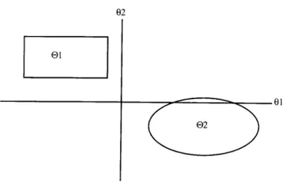
FIG. 1. The support of the posterior distribution is the set O = 0 1 u 0 2 , which is disconnected.

This form of the algorithm is due to Hastings (1970). The Metropolis et al. (1953) form takes q(Ocm',O*) = q ( 8 * , d m ' ) . A simple variant that is often useful is the independence chain (Tierney, 1994), whereby q ( d m i , 6 ' ) = k(€"). Then

cc(dm', 6') = min p(e*IyT, A) k ( d m ' ) ~ ( e ' ~ ' l ~ ~ , A) k(e')

where w(0) = p ( ~ I ~ T , ~ ) / k ( 0 ) . The independence chain is closely related to acceptance sampling and importance sampling. In acceptance sampling, if the posterior density is low (high) relative to the source density, then the probability of acceptance is low (high). In importance sampling, if the posterior density is low (high) relative to the importance sampling density, then the weight assigned to the draw is low (high). In the independence chain, to the extent the posterior density is lower (higher) relative to the proposal than was the case in the previously accepted draw, the prob- ability of accepting the proposed vector is lower (one).

There is a simple two-step argument that motivates the convergence of the sequence

{dm')

generated by the Hastings-Metropolis algorithm to the posterior. (This approach is due to Chib and Greenberg, 1995.) First, observe that if the transition probability function p ( d m i ,

dm+")

satisfies the reversibility condition

for stated p ( . ) , then it has p ( . ) as an invariant distribution. To see this, note that if (3.4.1) holds. then

Second, establish that the Hastings-Metropolis algorithm satisfies the reversibility condition. For

dm"'

=

d m ) ,

(3.4.2) is satisfied trivially. For

dm"'

# d m ' , suppose without loss of generality that p ( ~ ~ m " ~ ) / q ( 8 ' m ' . B("~")

>

p(~'"')/q(d"'+l', d m ' ) . Then

and

whence (3.4.2) is satisfied.

In implementing the Hastings-Metropolis algorithm, the transition probability density func- tion must share two important properties. First, it must be possible to generate 8' efficiently from q(@"', 0 ' ) . A second key characteristic of a satisfactory transition process is that the uncon- ditional acceptance rate not be so low that the time required to generate a sufficient number of distinct

dm)

is too great.

In the case of the independence chain, the Hastings-Metropolis algorithm will be efficient under essentially the same conditions that the corresponding importance sampling algorithm with the same j(8) will be efficient. If there are values of 8 for which p * ( 8 1 ~ , , A)/j(19) is very much greater than at other values, then the importance sampling algorithm will place very high weights on these values, which are drawn infrequently relative to p ' ( ~ I ~ , , ~ ) . The Hastings-Metropolis independence chain will tend to remain at such values for many successive iterations. In either case, the RNE will, as a consequence, be low.

Another variant of the Hastings-Metropolis algorithm is the random walk chain, in which q ( d m ' . 8 * ) = f ( d m ' - 8') = f(0' - d m ' ) . For example, f could be multivariate normal, with mean

zero and a constant variance matrix. If the variance matrix is chosen to reflect the shape of p ' ( ~ I ~ , , ~ ) at least roughly, then this algorithm can be quite efficient.

3 . 5 Some M C M C Theory

Much of the treatment here draws heavily on the work of Tierney (1994), who first used the theory of general state space Markov chains to demonstrate convergence, and Roberts and Smith

(1994), who elucidated sufficient conditions for convergence that turn out to be applicable in a wide variety of problems in econometrics.

Let

{e(mJ}I=o

be a Markov chain defined on 0 ' R h i t h transition density K : O x O

+

3

'

such that, for all v-measurable 0,, 0 ,

where

The transition density K is substochastic: it defines only the distribution of accepted candi- dates. Assume that K has no absorbing states so that r(8) < 1 V 8 E 0 . The corresponding substochastic kernel over m steps is then defined iteratively,

This describes all m-step transitions that involve at least one accepted move. As a function of d m ) , ~ ~ " ' ( 8 ~ ~ " , .

)

is the p.d.f. with respect to v of o""~, excluding realizations with 8'") = 8'') V n = I,

.

.

.

, m . For any v-measurable 0 , , let ~ ( " ' ( 8 ( ~ ' , 0,) denote the m'th iterate of P ,

An invariant distribution of the transition density K is a function p(8) that satisfies

for all v-measurable 0 , . Let 0' = (8 E 0 : p(8) > 0). The density K is p-irreducible if for all

do'

E O * , P(o,,) > 0 implies that P'"'(B(O~, 0,)

>

0 for some m >1. Return to Figure 1, where the support is disconnected and the Markov chain is the Gibbs sampler. Note that if

do)

E

6,,

it is impossible that 8'") E

6 ,

( j # i, any m > 0). Thus, the transition density is not irreducible in this case. There are two invariant distributions, one for

0,

(reached if

do)

E

6,)

and one for

G2

The transition density K is aperiodic if there exists no v-measurable partition

O =

U:I:6,

( r

>

2 ) such that

It is Harris recurrent if P

[

dm'

t 0, i.o./d0)] = 1 for all V-measurable 0, with

L

_{p(Q)dv(Q) > 0} and all 8") E 0 . l 7 It follows directly that if a kernel is Harris recurrent, then it is p-irreducible. A kernel whose invariant distribution is proper, and that is both aperiodic and Harris recurrent, is ergodic by definition (Tierney, 1994, 1712-1713).

A useful metric in what follows is the total variation norm for signed and bounded measures

p defined over the field of all V-measurable sets S, on 0 : 11p/1= sup ,,,,,

40,)

- inf

,,,,,"

~ ( 0 , ) . Theorem 3.5.1. Convergence of continuous state Markov chains. Suppose

~(BIY,,

A) is an invariant distribution of the transition density K ( B , ~ * ) .

(a) If K is ~(o~Y,,A)-irreducible, then ~ ( ~ I Y , , A ) is the unique invariant distribution. (b) If K is ~(~IY,,A)-irreducible and aperiodic, then except possibly for

o'~')

in a set of posterior probability zero, I ~ P ' ~ ' ( B ' ~ " , ) - P ( ~ Y , . A)Il i 0 .

If K is ergodic (that is, it is also Harris recurrent), then this occurs for all @ .

(c) If K is ergodic with invariant distribution ~(BIY,, A ) , then for all g(Y,,8) absolutely integrable with respect to

~(oIY,,

A) and for all 8'" E 0 ,

ProoJ: (a) and (b) follow immediately from Theorem 1 and (c) from Theorem 3 in Tierney

(1994). ##

For the Gibbs sampling algorithm, Section 3.3 argues informally that

~ ( ~ I Y , , A )

is an invariant distribution. More formally, (3.3.2) implies that for the blocking 0' = (Q;,,,

e;,),

he

expression L O . ~n P

1

13 ("'I E 0 -

,,

I . o

.I

8'"'

]

- - 1 means mfinitely often. The condition is that ~ i r n , + ~ ~ [ ~ M , X ~ , ( e ' , ~ " ) 5 L] =

o

v L