Discrete optimization methods to fit piecewise affine models to data points

Discrete optimization methods to fit piecewise affine

models to data points

E. Amaldia_{, S. Coniglio}b,1_{, L. Taccari}a a_{Dipartimento di Elettronica, Informazione e Bioingegneria,}

Politecnico di Milano

Piazza Leonardo da Vinci 32, 20133 Milano, Italy b_{Department of Mathematical Sciences}

University of Southampton

University Road, Southampton, SO17 1BJ, UK

Abstract

Fitting piecewise affine models to data points is a pervasive task in many

scien-tific disciplines. In this work, we address thek-Piecewise Affine Model Fitting

with Piecewise Linear Separability problem(k-PAMF-PLS) where, given a set

ofmpoints{a1, . . . ,am} ⊂Rnand the corresponding observations{b1, . . . , bm} ⊂

R, we have to partition the domainRn intokpiecewise linearly (or affinely) sep-arable subdomains and to determine an affine submodel (function) for each of them so as to minimize the total linear fitting error w.r.t. the observationsbi.

To solve k-PAMF-PLS to optimality, we propose a mixed-integer linear

programming (MILP) formulation where symmetries are broken by separating shifted column inequalities. For medium-to-large scale instances, we develop a four-step heuristic involving, among others, a point reassignment step based on the identification of critical points and a domain partition step based on multi-category linear classification. Differently from traditional approaches proposed in the literature for similar fitting problems, in both our exact and heuristic methods the domain partitioning and submodel fitting aspects are taken into account simultaneously.

Computational experiments on real-world and structured randomly gener-ated instances show that, with our MILP formulation with symmetry breaking constraints, we can solve to proven optimality many small-size instances. Our four-step heuristic turns out to provide close-to-optimal solutions for small-size instances, while allowing to tackle instances of much larger size. The experi-ments also show that the combined impact of the main features of our heuristic

Email addresses: [email protected](E. Amaldi),[email protected](S. Coniglio),[email protected](L. Taccari)

1_{The work of S. Coniglio was carried out, for a large part, while he was with Dipartimento} di Elettronica, Informazione e Bioingegneria, Politecnico di Milano and with Lehrstuhl II f¨ur Mathematik, RWTH Aachen University, supported. While with the latter, he was supported by the German Federal Ministry of Education and Research (BMBF), grant 05M13PAA, and Federal Ministry for Economic Affairs and Energy (BMWi), grant 03ET7528B.

is quite substantial when compared to standard variants not including them. We conclude with an application to the identification of dynamical piecewise affine systems for which we obtain promising results of comparable quality with those achieved with state-of-the-art methods from the literature on benchmark data sets.

————————————————————————— 1. Introduction

Fitting a set of data points in Rn with a combination of low complexity

models is a pervasive problem in, essentially, any area of science and engi-neering. It naturally arises, for instance, in prediction and forecasting when determining a model to approximate the value of an unknown function, or whenever one wishes to approximate a highly complex nonlinear function with a simpler one. Applications range from optimization (see, e.g., [TV12] and the references therein) to statistics (see, e.g., the recent work in [BM14]), to data mining (see, e.g., [AM02, BS07]), and to system identification (see, for instance, [FTMLM03, BGPV05, TPSM06]), only to cite a few.

Among the different options,piecewise affine modelshave a number of

advan-tages with respect to other model fitting approaches. Indeed, they are compact and simple to evaluate, visualize, and interpret, in contrast to models obtained with other techniques such as, e.g., neural networks, while allowing to approxi-mate even highly nonlinear functions.

Given a set of m points A = {a1, . . . ,am} ⊂ Rn, with index set I =

{1, . . . , m_}, with the corresponding observations {b1, . . . , bm} ⊂R and a posi-tive integerk, the general problem of fitting a piecewise affine model to the data points{(a1, b1), . . . ,(am, bm)}consists in partitioning the domainRnintok con-tinuoussubdomainsD1, . . . , Dk, with index setJ ={1, . . . , k}, and in

determin-ing, for each subdomainDj, anaffine submodel(an affine function)fj:Dj→R,

so as to minimize a measure of the total fitting error. Adopting the notation2

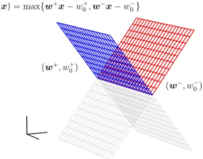
fj(x) =wjx−w j

0 with coefficients (wj, w j

0)∈Rn+1, the j-th affine submodel

corresponds to the hyperplaneHj ={(x, fj(x))∈Rn+1 :fj(x) =wjx−wj0}

where x _∈ Dj. The total fitting error is defined as the sum, over all i ∈ I,

of a function of the difference between bi and the valuefj(i)(ai) provided by

the piecewise affine model, wherej(i) is the index of the affine submodel

corre-sponding to the subdomainDj(i) which contains the pointai.

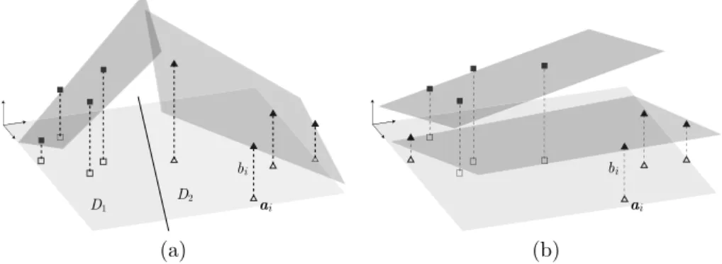
In the literature, different error functions (e.g., linear or quadratic) as well as different types of domain partition (with linearly or nonlinearly separable subdomains) have been considered. See Figure 1 (a) for an illustration of the

case withk= 2 and a domain partition with linearly separable subdomains.

2_{For greater readability, transposition symbols will be omitted throughout the paper. If} one wanted to specify the row and column nature of the vectors that we use,aiwould be a

bi ai D 1 D₂ bi ai (a) (b)

Figure 1: (a) A piecewise affine model withk= 2, fitting the eight data pointsA={ai}i∈I

and their observations{bi}i∈Iwith two submodels (in dark gray). The points (ai, bi) assigned

to each submodel are indicated byandN. The model adopts a linearly separable partition

of the domainR2(represented in light gray). (b) An infeasible solution obtained by solving a k-hyperplane clustering problem inR3 withk= 2. Although yielding a smaller fitting error

than that in (a), this solution induces a partitionA1, A2ofAwhere the pointsaiassigned to

the first submodel (indicated by) cannot be linearly separated from those assigned to the

second submodel (indicated byM). In other words, the solution does not allow for a domain partitionD1, D2 ofR2 with linearly separable subdomains that is consistent with the point partitionA1, A2.

In this work, the focus is on the version of the general piecewise affine model

fitting problem with a linear error function (`1 norm) and a domain

parti-tion with piecewise linearly3 _{separable subdomains. We refer to it as to the}

k-Piecewise Affine Model Fitting with Piecewise Linear Separability problem

(k-PAMF-PLS). A more formal definition of the problem will be provided in

Section 3.

k-PAMF-PLS shares a connection with the so-calledk-Hyperplane

Cluster-ing problem (k-HC), an extension of a classical clustering problem which calls

for k hyperplanes in Rn+1 which minimize the sum, over all the data points

{(a1, b1), . . . ,(am, bm)}, of the `2 distance from (ai, bi) to the hyperplane the

point is assigned to. See [BM00, AC13, Con11, Con15] for some recent work on the problem and [ADC13] for the problem variant aiming at minimizing the number of hyperplanes needed to fit all the points within a prescribed toler-anceε >0.

It is nevertheless crucial to note that, differently from many of the approaches in the literature (which we briefly summarize in Section 2) and depending on the type of the domain partition that is adopted, a piecewise affine function

cannot be determined by just solving an instance ofk-HC. A naive application

of algorithms designed for k-HC to tackle k-PAMF-PLS can indeed lead to

solutions with a large fitting error, as a consequence of the domain partitioning

3_{Although this kind of separation employs piecewise affine functions, it is usually referred} to, in the literature, aspiecewise linear. We will do so also here for uniformity with previous work.

aspect being entirely neglected. As illustrated in Figure 1 (b), the two aspects

of k-PAMF-PLS, namely, submodel fittingand domain partitioning, should be

taken into account at once to obtain a solution where the two are consistent. For this reason, most of the algorithms in the literature incorporate techniques to enforce the piecewise linear separability of the domain, typically after first solvingk-HC (or one of its variants). In this work, we propose exact methods for

k-PAMF-PLS based on mixed-integer linear programming as well as heuristic

algorithms which consider both aspects of the problem simultaneously, rather than deferring the domain partitioning aspect to a later stage of the solution process.

The paper is organized as follows. After summarizing previous and related works in Section 2, we formally define the problem under consideration in Sec-tion 3. In SecSec-tion 4, we provide a Mixed-Integer Linear Programming (MILP)

formulation fork-PAMF-PLS. We then strengthen the formulation when using

it for solving the problem in a branch-and-cut setting by generating symmetry-breaking constraints. In Section 5, we propose a four-step heuristic to tackle larger-size instances. Computational results are reported and discussed in

Sec-tion 6. In SecSec-tion 7, we consider the applicaSec-tion ofk-PAMF-PLS to problems

in the area of dynamical system identification and compare the obtained re-sults with those provided by state-of-the-art methods. Section 8 contains some concluding remarks. Portions of this work appeared, in a preliminary stage, in [ACT11, ACT12].

2. Previous and related work

Recently, there has been a growing interest in mixed-integer programming and discrete optimization approaches to a wide range of problems in the areas of data mining and statistics, see, e.g., [IR03, CSK06, BS07, CBR12, BM14, MT15]. As to the problem of fitting a piecewise affine model to data points, many variants have been considered in the literature. We briefly mention some of the most relevant ones in this section.

In some works, the domain is partitioned a priori, exploiting the

domain-specific information about the dataset at hand. This approach has a typically limited applicability, as it requires knowledge of the underlying structure of the data, which may often not be available. For some examples, the reader is referred to [TV12] (which admits the use of a predetermined domain partition as a special case of a more general approach) and to the references therein.

In other works, a domain partition is easily derived when the attention is restricted to convex or concave piecewise affine models. Indeed, if the model is

convex, each subdomainDj is uniquely defined as Dj ={x∈Rn : fj(x) ≥

fj0(x)∀j0 ∈ J} (similarly, for concave models, with ≤ instead of ≥). This is,

for instance, the case of [MB09] and [MRT05], where the fitting function is the

pointwise maximum (or minimum) of a set ofkaffine functions. In the case of

hinging hyperplane models, see [Bre93] or [RBL04] and the references therein, the domain partition does not need to be explicitly derived due to the special structure of this type of piecewise affine models.

In more general versions of the problem, a partition of the domain has to be explicitly derived together with the fitting submodels in order to obtain a

piecewise affine function from Rn to R. To the best of our knowledge, most

of the available methods aretwo-phase in nature, in that they split the

prob-lem into two subprobprob-lems that are solved sequentially: i) aclustering problem

aiming at partitioning the data points and simultaneously fitting each subset

with an affine submodel, and ii) a classification problem asking for a domain

partition consistent with the previously determined submodels and the corre-sponding point partition. Note that the clustering problem considers the data points_{(a1, b1), . . . ,(am, bm)} ⊂Rn+1, whereas the classification problem con-siders the original points_{a1, . . . ,am} ⊂Rn but not the observations bi. The

clustering phase is typically carried out by either choosing a given numberkof

hyperplanes which minimize the fitting error, or by finding a minimum number

of hyperplanes yielding a fitting error of, at most, a given ε. Although such

two-phase approaches turn out to perform satisfactorily in several of the control applications that are cited in this section, in the general case they may lead to solutions with a large fitting error (due to deferring the domain partition to the end), as also illustrated in Section 6 with our computational experiments.

Among the two-phase methods available in the literature, we first mention [BGPV05], which includes a postprocessing phase aiming at enforcing piecewise linear separability. In its clustering phase, as proposed in [AM02], the problem

of fitting the data points inRn+1 with a minimum number of linear submodels

within a given error tolerance ε > 0 is formulated and solved as a Min-PFS

problem, which amounts to partitioning a given infeasible linear system into a minimum number of feasible subsystems. Then, in the classification phase,

the domain is partitioned via aSupport Vector Machine(SVM). In [TPSM06]

the authors solve ak-hyperplane clustering problem via the heuristic proposed

in [BM00], resorting to SVM for the classification phase. A similar approach

is also adopted in [BS07], where, in the first phase, a k-hyperplane clustering

problem is solved as a mixed-integer linear program and, in the second phase,

the domain partition is derived viaMulticategory Linear Classification(MLC).

For references to SVM and MLC, see [Vap96] and [BM94], respectively. The

method proposed in [FTMLM03] associates, to each data point ai, a

hyper-plane computed by solving a least square problem over thecclosest points, and

then clusters them into k groups via a weighted version of the k-means

algo-rithm4 _{[Mac67]. To avoid grouping together hyperplanes corresponding to far}

away points and, thus, partially accounting for the domain partitioning aspect,

clustering is carried out in a 2n+ 1-dimensional feature space which includes

the hyperplane parameters and the centroid of the c points corresponding to

the neighbourhood. Finally, SVM is applied to derive the domain partition a

posteriori.

4_{k-means is a well-known heuristic to partitionmpoints{a}

1, . . . ,am}intokgroups

(clus-ters) so as to minimize the total distance between each point and the centroid (mean) of the corresponding group.

Note that, in several of the cited articles, the authors also propose heuristics

to select a suitable number k of submodels which, in our work, we assume to

be given. In Subsection 6.6, we will give an idea on how to estimate a suitable

value forkusing a cross-validation technique.

As already mentioned in the previous section, these two-phase approaches may produce, in the first phase, affine submodels inducing a partitionA1, . . . , Ak

of the points of A which does not allow for a consistent domain partition

D1, . . . , Dk, i.e., for a partition where all the pointsai in a subset Aj are

con-tained into one and only one subdomainDj(i). Refer again to Figure 1 (b) for

an illustration.

A large body of work on problems related to piecewise affine model fitting has been carried out in the context of dynamical system identification for the case

of so-called hybrid systems. Many approaches typically encompass two-phase

heuristic methods such as those in [BGPV05, TPSM06, FTMLM03], which we have already mentioned. A few mixed-integer programming formulations have also been proposed for similar fitting problems. In the case of switched system identification, such as in [PJFTV07, MK05], the focus is on finding an optimal assignment of the points to the submodels without determining the domain partition. In the case of hinging hyperplane models [Bre93, RBL04], no explicit domain partition needs to be derived. Another line of research is that pursued in, among others, [OL13, OSLC12], where the authors consider sparse optimization approaches aiming at the identification of piecewise affine models with a trade-off between number of pieces and fitting error. For further details on similar applications and methodologies, we refer the reader to the surveys [PJFTV07, GPV12], as well as to Section 7.

3. Problem definition

In this work, we require that the domain partitionD1, . . . , Dk ofRn satisfy

the property ofpiecewise linear separability, which forms the basis of

multicat-egory linear classification[BM94]. In the following, we briefly recall some key

features of this well-known classification paradigm, which we will then leverage in the remainder of the paper.

3.1. Piecewise linear separability and multicategory linear classification Given k groups of points A1, . . . , Ak ⊂ Rn, the multicategory linear

clas-sification problem calls for a partition of the domain Rn into k subdomains

D1, . . . , Dk which, as shown in [DF66] (also see [BM94]) can be defined by

introducing, for each group of points Aj with j ∈ J, a vector of parameters

(yj_{, y}j

0)∈Rn+1 such that a pointai∈Aj belongs to the subdomain Dj if and

only if, for everyj0 ₆=j, we have (yj −yj0

)ai−(yj0−y j0

0)>0. This equivalently

amounts to imposing that, for any pair of indicesj1, j2 ∈J withj1 6=j2, the

sets of pointsAj1 andAj2 are separated by the hyperplaneHj1j2 ={x∈R

n _: (yj1−_yj2_{)x = y}j1 0 −y j2 0 } with coefficients (y j1 −_yj2_{, y}j1 0 −y j2 0 ) ∈ R n+1_{, see}

D1 D2 D3 D4 D5 D1 D2 (a) (b)

Figure 2: (a) Piecewise linear separation of five linearly separable groups of points. (b) Classification with a minimum misclassification error of two linearly inseparable groups of points (note the misclassified black point).

Figure 2 (a) for an illustration. It follows that, for anyj_∈J, the domainDj is

defined as: Dj= n x∈Rn: (yj−yj 0 )x−(yj₀₋y₀j0)>0 ∀j0_∈J_{\ {}j0_}o. (1) If the group of pointsA1, . . . , Ak are not piecewise linearly separable, there

exists at least a pointaiand a pairj1, j2for which the inequality (yj1−yj2)ai−

(yj1

0 −y j2

0 ) >0 is violated for any choice of the vectors of parameters (yj, y j 0)

with j _∈ J. In this case, the typical approach is to look for a solution which

minimizes the sum, over all the data points, of the so-calledmisclassification

error. For a point ai ∈ Aj(i), where j(i) is the index of the group the point

belongs to, the misclassification error is defined as: max 0, max j∈J\{j(i)} n −(yj(i) −yj_)a i+ (y j(i) 0 −y j 0) o , (2)

thus corresponding to the largest violation among the inequalities (yj(i) −yj_)a

i−

(yj(i)_{0 −}yj₀)>0. For an illustration, see Figure 2 (b). Since the set of vectors (yj_{, y}j

0), for j ∈ J, satisfying constraint (yj(i)− yj_)a

i−(y j(i) 0 −y

j

0)>0 is an open subset ofRn+1, it is common practice to replace

the constraint by the inhomogeneous constraint (yj(i)

−yj_)a i−(y j(i) 0 −y j 0)≥1,

which induces a closed feasible set. This can be done without loss of generality if we assume that the norm of the vectors (yj(i)_yj(i)

0 ) and (yj, y j

0) can be arbitrarily

large, for all j _∈ J. Indeed, if (yj(i)

−yj_)a i−(y j(i) 0 −y j 0) > 0 but (yj(i)− yj_)a i−(y j(i) 0 −y j

0)<1 for someai∈ A, then a feasible solution which satisfies

the inhomogeneous constraint can be obtained by just scaling (yj(i)_{, y}j(i)

0 ) and (yj_{, y}j 0) by a constantλ≥ 1 (yj(i)_−yj_)a i−(yj0(i)−y j 0)

. The misclassification error for the inhomogeneous version is thus:

max 0, max j∈J\{j(i)} n 1₋(yj(i) −yj_)a i+ (y j(i) 0 −y j 0) o . (3)

3.2. k-Piecewise affine model fitting problem with piecewise linear separability

We can now provide a formal definition of the k-Piecewise Affine Model

Fitting with Piecewise Linear Separability problem.

k-PAMF-PLS: Given a set of m points _A = _{a1, . . . ,am} ⊂ Rn

with the corresponding observations_{b1, . . . , bm} ⊂Rand a positive integerk:

i) partition _Ainto k subsetsA1, . . . , Ak which are piecewise

lin-early separable via a domain partition D1, . . . , Dk of Rn

in-duced, according to Equation (1), by a set of vectors (yj_{, y}j 0)∈

Rn+1, forj∈J,

ii) determine, for each subdomainDj, an affine functionfj :Dj →

Rwherefj(x) =wjx−w j 0 with parameters (w j_{, w}j 0)∈R n+1_,

so as to minimize the linear error function

m X i=1 bi− wj(i)ai−w j(i) 0 ,

wherej(i)_∈J is the index for whichai∈Aj(i)⊂Dj(i).

It is worth emphasizing that, in this problem, both the domain partition and the fitting hyperplanes have to be determined jointly.

4. Strengthened mixed-integer linear programming formulation

In this section, we propose an MILP formulation to solve k-PAMF-PLS

to optimality via a branch-and-cut method, as implemented in state-of-the-art MILP solvers. To enhance the efficiency of the solution algorithm, we break the symmetries that naturally arise in the formulation by generating symmetry-breaking constraints, as we will explain in the following.

Our MILP is derived by combining an adapted hyperplane clustering for-mulation with a multicategory linear classification one. The former allows us

to partition the data points into k subsets A1, . . . , Ak and to determine an

affine submodel for each of them (see, e.g., [AC13] or [MK05, PJFTV07] for closely related formulations for the identification of switched systems). The latter guarantees a piecewise linearly separable domain partition D1, . . . Dk,

consistent with theksubsetsA1, . . . , Ak (see the previous section and [BM94]).

Consistently with the definition of the problem, in the resulting formulation, the parameters of the fitting affine submodels and the piecewise linear domain

partition are determinedsimultaneously.

4.1. MILP formulation

For each i _∈I and j _∈ J, we introduce a binary variable xij which takes

value 1 if the point ai is contained in the subset Aj and 0 otherwise. Let zi

be the fitting error of point ai ∈ A for each i ∈ I, (wj, wj0) ∈ R

n+1 _{be the}

parameters of the submodel of indexj_∈J, and (yj_{, y}j

0)∈Rn+1, withj∈J, be

M2be large enough constants (whose value is discussed below). The formulation is as follows: min m X i=1 zi (4) s.t. k X j=1 xij= 1 ∀i∈I (5) zi≥bi−wjai+w0j−M1(1−xij) ∀i∈I, j∈J (6) zi≥ −bi+wjai−wj0−M1(1−xij) ∀i∈I, j∈J (7) (yj1_−yj2_)a i−(yj01−y j2 0 )≥1−M2(1−xij1) ∀i∈I, j1, j2∈J:j16=j2 (8) xij∈ {0,1} ∀i∈I, j∈J (9) zi≥0 ∀i∈I (10) (wj, wj0)∈R n+1 ∀j∈J (11) (yj, yj₀)∈Rn+1 ∀j∈J. (12)

Constraints (5) guarantee that each point ai ∈ A be assigned to exactly one

submodel. Constraints (6) and (7) impose thatzi=|bi−wj(i)ai+w j(i) 0 |. This

is because, together, they imply that zi ≥ |bi−wjai +wj0| −M1(1−xij).

Whenxij = 1, this amounts to imposingzi ≥ |bi−wjai+wj0| (which will be

tight in any optimal solution due to the objective function direction), whereas

it becomes redundant (sincezi≥0) when xij = 0 andM1is large enough. For

eachj1 ∈J, Constraints (8) impose that all the points assigned to the subset

Aj1 (for which the term −M2(1−xij) vanishes) belong to the intersection of all the halfspaces defined by (yj1−yj2)a

i−(y j1

0 −y j2

0 )≥1, whereas they are

deactivated when xij1 = 0 and M2 is sufficiently large. This way, we impose

a zero misclassification error for each data point, thus guaranteeing piecewise linear separability among the points assigned to the different submodels. Note that, if Constraints (8) are dropped, we obtain a relaxation corresponding to

a k-hyperplane clustering problem where the objective function is measured

according to (4), (6), and (7).

It is important to observe that, in principle, there exists no (large enough)

finite value for the parameterM1 in Constraints (6) and (7). As an example,

the fitting error between a point (a, b) = (e,₋1)∈Rn+1, whereeis the all-one vector, and the affine functionf =wa−1 is equal tokwk1(the`1norm ofw)

and, thus, it is unbounded and arbitrarily large for an arbitrarily large kwk1. Letj(i)∈J such thatxij(i) = 1. The introduction of a finiteM1 corresponds

to letting: zi= max        j=j(i) andx_ij(i)=1 z }| { |bi−wj(i)ai+w j(i) 0 |, j6=j(i) andxij=0 z }| { max j∈J\{j(i)}{|bi−w j_a i+w j 0| −M1}        , (13)

rather than zi = |bi−wj(i)ai+w j(i)

penalization term into the objective function equal to: m X i=1 max 0, max j∈J\{j(i)}{|bi−w j_a i+w0| −j M1} − |bi−wj(i)ai+w j(i) 0 | . (14)

The effect is of penalizing solutions where the fitting error betweenany point

andanysubmodel is too large, regardless of the submodels to which each point

is assigned.

We face a similar issue with Constraints (8) due to the presence of the pa-rameterM2. Indeed, for any finiteM2and forxij1 = 0, each of such constraints implies (yj1_−yj2_)a

i−(yj01 −y j2

0 )≥ 1−M2. Hence, Constraints (8) impose

that thelinear distance5

−(yj1−_yj2_)a

i+ (y j1

0 −y j2

0 ) (notice that the signs are

consistent with Equation (3)) between each pointai and the hyperplane

sepa-ratinganypair of subdomainsDj1, Dj2 be smaller thanM2−1 even ifaiis not contained in either of the subdomains, i.e., even ifai ∈/ Aj1 andai∈/Aj2.

In spite of the lack of theoretically finite values for M1 and M2, setting

them to a value a few orders of magnitude larger than the size of the box

encapsulating the data points inRn+1typically suffices to produce good quality

(if not optimal) solutions. We will mention an occurrence where this is not the case in Section 6.

4.2. Symmetries

LetX _{∈ {}0,1_}m×k _{be the binary matrix with entries}

{X_}ij =xij fori∈I

andj_∈J. We observe that Formulation (4)–(12) admits symmetric solutions as

a consequence of the existence of a symmetry group acting on the columns ofX.

This is because, for anyXrepresenting a feasible solution, an equivalent solution

can be obtained by permuting the columns ofX, an operation which corresponds

to permuting the labels 1, . . . , k by which the submodels and subdomains are

indexed.

From a computational point of view, the solvability of our MILP

formu-lation for k-PAMF-PLS is hindered by the existence of symmetries. On the

one hand, this is because, when adopting methods based on branch-and-bound, symmetries typically lead to an unnecessarily large search tree where equiva-lent (symmetric) solutions are discovered again and again at different nodes. On the other hand, the presence of symmetries usually leads to weaker Lin-ear Programming (LP) relaxations, for which the barycenter of each set of symmetric solutions, which often yields very poor LP bounds, is always fea-sible [KP08]. This is the case of our formulation where, for a sufficiently large M =M1 =M2 ≥ _k−k₁max{1,|b1|,|b2|, . . . ,|bm|}, the LP relaxation of

Formu-lation (4)–(12) admits a solution of value 0. To see this, let xij = _k1 for all

i_∈I, j_∈J. Constraints (5) are clearly satisfied. Let thenzi = 0 for alli∈I,

5_{Given a pointaand a hyperplane of equationwx−w}

0= 0, the distance fromato the closest point belonging to the hyperplane amounts to |wa_kw−_kw0|

2 . Then, thelinear distance

(wj_{, w}j

0) = (0,0) and (y j_{, y}j

0) = (0,0) for allj∈J. Constraints (6), (7), and (8)

are then satisfied whenever we have, respectively,M1k−_k1 ≥bi, M1k−_k1 ≥ −bi,

andM2k−_k1 ≥1.

A way to deal with this issue is to partition the set of feasible solutions into equivalence classes (ororbits) under the symmetry group, selecting a single representative per class. Different options are possible. We refer the reader to [Mar10] for an extensive survey on symmetry in mathematical programming. A possibility, originally introduced in [MDZ01, MDZ06], is of selecting as a representative the (unique) feasible solution of each orbit where the columns

ofX are lexicographically sorted in nonincreasing order. According to [KP08],

we call the convex hull of such lexicographically sorted matricesX_{∈ {}0,1_}m×k

orbitope.

4.3. Symmetry breaking constraints from the partitioning orbitope

Since, in our case,X is apartitioning matrix(a matrixX_{∈ {}0,1_}m×k _with

exactly a 1 per row), we are interested in the so-called partitioning orbitope,

whose complete linear description is given in [KP08].

Neglecting the trivial constraints, the partitioning orbitope is defined by the

set of so-called Shifted Column Inequalities (SCIs). Call B(i,j) a bar, defined

as B(i,j) = {(i, j),(i, j + 1), . . . ,(i,min{i, k})}, and col(i,j) a column, defined

as col(i,j) ={(j, j),(j+ 1, j), ...,(i, j)}. Intuitively, a shifted column S(i,j) is a

subset of the indices of X obtained by shifting some of the indices in col(i,j)

diagonally towards the upper-left portion of X. More formally, for a pair of

indices (i, j), a shifted column S(i,j) is a collection of indices in I ×J such

that S(i,j)={(c1, c1),(c2+ 1, c2), . . . ,(cη+η−1, cη)} with η =i−j+ 1 and

1 _≤ c1 ≤ c2· · · ≤ cη ≤ j. For c1 = · · · = cη = j, we obtain the original

(nonshifted) columncol(i,j). For an illustration, see Figure 3. For two subsets

of indicesB(i,j), S(i−1,j−1)⊂I×J thus defined, an SCI reads:

X (i0_,j0_)∈B (i,j) xi0_j0 − X (i0_,j0_)∈S (i−1,j−1) xi0_j0 ≤0.

As shown in [KP08], the linear description of the partitioning orbitope is: k X j=1 xij= 1 ∀i∈I (15) X (i0_,j0_)∈B (i,j) xi0_j0− X (i0_,j0_)∈S (i−1,j−1) xi0_j0 ≤0 ∀B_(i,j), S_(i−1,j−1):i, j∈J, i, j≥2 (16) xij= 0 ∀i∈I, j∈J:j≥i+ 1 (17) xij≥0 ∀i∈I, j∈J, (18)

where Constraints (16) are SCIs, while Constraints (17) restrict the problem to

the only elements ofX that are either on the main diagonal or below it.

Although there are exponentially many SCIs, the corresponding separa-tion problem can be solved in linear time by dynamic programming, as shown in [KP08].

i j η i j i j (a) (b) (c)

Figure 3: (a) The barB(i,j) (in black and dark gray) and the column col(i−1,j−1)(in light gray). (b) and (c) Two shifted columns (in light gray) obtained by shifting col(i−1,j−1). Note how the shifting operation introduces empty rows.

When solving the MILP formulation (4)–(12) with a branch-and-cut algo-rithm, we generate maximally violated SCIs both at each node of the enumera-tion tree (by separating the corresponding fracenumera-tional soluenumera-tion) and every time a new integer solution is found (thus separating the integer incumbent solution). 5. Four-step heuristic algorithm

As we will see in Section 6, the introduction of SCIs has a remarkable impact on the solution times. Nevertheless, even with them, the MILP formulation only allows for the solution of small to medium size instances in a reasonable amount of computing time.

To tackle instances of larger size, we propose an efficient heuristic that takes into account, at each iteration, all the three aspects of the problem, namely, affine submodel fitting, point partition, and domain partition. At each itera-tion, the heuristic alternately and coordinately carries out a sequence of four steps, the last two of which guarantee that the current solution always admits a piecewise linear domain partition. Before describing the details of the four steps, it is worth pointing out that the structure of our algorithm differs from other heuristics (such as [BGPV05, FTMLM03]) where the domain partitioning aspect is considered directly just once, in the very last iteration. Moreover, our method does not amount to just running an off-the-shelf clustering algorithm (tackling the first and second aspects of the problem) until convergence to a local minimum, deriving a domain partition, and then feeding a refined solution again to the clustering method as a warm start.

We start from a feasible solution composed of a point partitionA1, . . . , Ak, a

domain partitionD1, . . . , Dk(induced by the parameters (yj, y0j) forj∈J), and

a set of affine submodels of parameters (wj_{, w}j

0), for j∈J. At each iteration,

the algorithm tries to improve the current solution by applying the following four steps (until convergence or until a time limit is met):

i) Submodel Fitting: Given the current point partitionA1, . . . , Ak ofA=

param-eters (wj_{, w}j

0) which minimizes the linear fitting error over all the data

points{(a1, b1), . . . ,(am, bm)} ⊂Rn+1. As we shall see, this is carried out by solving a single linear program.

ii) Point Partition: Given the current set of affine submodelsfj:Dj→R

with fj(x) = wjx−w j

0 and j ∈J, identify a set of criticaldata points

(ai, bi) ∈ Rn+1 and (re)assign them to other submodels in an attempt

to improve (decrease) the total linear fitting error over all the dataset. As described below, the identification and reassignment of such points is

based on anad hoccriterion and on a related control parameter.

iii) Domain Partition: Given the current point partitionA1, . . . , Ak ofA=

{a1, . . . ,am}, a multicategory linear classification problem is solved via

linear programming to either find a piecewise linearly separable domain partitionD1, . . . , Dk ofRnconsistent with the current point partition or, if none exists, to construct a domain partition which minimizes the total misclassification error. In the latter case, i.e., when there is at least an in-dexj_∈Jfor whichAj6⊂Dj, we say that the previously constructed point

partition is notconsistentwith the resulting domain partitionD1, . . . , Dk.

iv) Partition Consistency: If the current point partition and domain

par-tition are inconsistent, the former is modified to make it consistent with

the latter. For every indexj _∈J and every misclassified pointai (if any)

belonging toAj(i.e., for anyai∈ Awhereai∈Ajandai∈Dj0, for some

j, j0 _{∈ J such that j 6=j}0_{), a}

i is reassigned to the subset Aj0 associated

withDj0.

We now describe the four steps in greater detail.

In theSubmodel Fittingstep, we determine, for eachj_∈J, the submodel

parameters (wj_{, w}j

0) yielding the smallest fitting error by solving the following

linear program: min m X i=1 di (19) s.t. di≥bi−wj(i)ai+w j(i) 0 ∀i∈I (20) di≥ −bi+wj(i)ai+w j(i) 0 ∀i∈I (21) (wj_{, w}j 0)∈R n+1 ∀j_∈J (22) di≥0 ∀i∈I, (23)

where j(i) denotes the submodel to which the point ai is currently assigned.

Note that this linear program, which is standard for solving regression problems

in`1-norm, decomposes intokindependent linear programs, one per submodel.

Let us now consider the Point Partition step. Many clustering

heuris-tics (see, e.g., [Mac67, BM00]) are based on the iterative reassignment of each

pointai to a subsetAj whose corresponding submodel yields the smallest

D₁ D₂ a₁ a_i b_i D₁ D₂ a₁ a_i b_i (a) (b)

Figure 4: (a) A solution corresponding to a local minimum for an algorithm where each point is reassigned to the submodel yielding the smallest fitting error. (b) An improved solution that can be obtained by reassigning the pointa1in (a) which, according to our criterion, achieves the highest ranking, to the rightmost submodel, and by updating the affine submodel fitting as well as the domain partition.

this choice is likely to lead to poor quality local minima. In our method, we adopt a criterion to help identify a set ofcritical pointswhich might jeopardize the overall quality of the current solution. The criterion is an adaptation of the one employed in the Distance-Based Point Reassignment heuristic (DBPR)

proposed in [AC13] for thek-hyperplane clustering problem.

The idea of the criterion is to identify as critical those points which not only give a large contribution to the total fitting error for their current submodel, but also have another submodel to which they can be reassigned without increasing too much the overall fitting error. The set of such points is determined by

ranking, for each subset Aj, each point ai ∈ Aj in nonincreasing order with

respect to the ratio between its fitting error w.r.t. the current submodel of

index j(i) and the fitting error w.r.t. a candidate submodel. The latter is

defined as the submodel that best fitsai but which is also different fromj(i).

Formally, for eachj_∈J, the criterion ranks each pointai∈Aj with respect to

the quantity: |bi−wj(i)ai+w j(i) 0 | minj∈J\{j(i)}{|bi−wjai+w j 0|}. (24)

ThePoint Partition step relies on acontrol parameter α_∈[0,1). Given

a current solution characterized by a point partition A1, . . . , Ak and the k

as-sociated affine submodels, letm(j) denote, for allj _∈J, the cardinality of Aj.

At each iteration and for each submodel of indexj_∈J,_dα m(j)_eof the points with highest rank are reassigned to the corresponding candidate submodel, even if this leads to a worse objective function value. The remaining points are sim-ply reassigned to the closest submodel (if they are not already assigned to it).

Then, α is decreased exponentially, by updating it as α := 0.99ρt, for some

parameter ρ _∈ (0,1), where t is the index of the current iteration. For an

illustration, see Figure 4 (b).

in-troduces a high variability in the sequence of solutions that are generated, the

search process is stabilized by decreasingα to 0 over the iterations, thus

pro-gressively shifting from introducing (for a large α) substantial changes in the

current solution to performing fine polishing operations (for a smallerα).

To avoid cycling effects, whenever a worse solution is found, we add the whole set of the point-to-submodel assignments that we carried out involving critical points to a tabu list of short memory. We also consider an aspiration criterion, that is, a criterion that allows to override the tabu status of a move if, by performing it, a solution with an objective function value that is better than that of the best solution found so far can be achieved. Since it is computationally too demanding to compute the exact objective function value of a solution obtained after the reassignment of a model from a submodel to another one (as

it would require to carry out theSubmodel Fitting, Domain Partition, and

Partition Consistencysteps for each point and at each iteration), we consider

a partial aspiration criterion in which we override the tabu status of a point-to-submodel reassignment only if the corresponding fitting error is strictly smaller than the value that was registered when the reassignment move was added to the tabu list.

In theDomain Partitionstep, we derive a domain partition by

construct-ing a piecewise linear separation of the sets A1, . . . , Ak which minimizes the

total misclassification error. This is achieved by solving a Multicategory Linear Classification problem via the linear program proposed in [BM94]:

min m X i=1 ei (25) s.t.ei≥ −(yj(i)−yj)ai+ (y j(i) 0 −y j o) + 1 ∀i∈I, j∈J\ {j(i)} (26) ei≥0 ∀i∈I (27) (yj, y₀j)∈Rn+1 ∀j∈J, (28)

where j(i) denotes the submodel to which the point ai is currently assigned,

and ei represents the misclassification error of point ai, for all i ∈ I. If this

subproblem admits an optimal solution with total misclassification error equal

to 0, then theksubsets are piecewise linearly separable. Otherwise, the current

solution contains at least a misclassified point ai ∈ Aj(i) with ai ∈ Dj for

j_∈J withj₆=j(i). Each such point is then reassigned toAj in thePartition

Consistencystep.

The overall four-step algorithm, which we refer to with the shorthand 4S-CR (4 Steps-4S-CRiterion), starts from a point assignment obtained by randomly generating the coefficients ofkaffine submodels and assigning each point (ai, bi)

to a submodel yielding the smallest fitting error (ties are broken arbitrarily).

The four steps are then repeated until α= 0, while storing the best solution

found so far. The method is then restarted until the time limit is reached.

Note that the Domain Partition step drives the search towards solutions

that induce a suitable domain partition, thus avoiding infeasible solutions which are good from a submodel fitting point of view but do not admit a piecewise

linearly separable domain partition, i.e., whereAj ⊂Dj does not hold for all

j _∈ J. Then, the Partition Consistency step makes sure that the point

partition and domain partition are consistent at the end of each iteration. 6. Computational results

In this section, we report and discuss on a set of computational results

ob-tained when solvingk-PAMF-PLS either to optimality with branch-and-cut and

symmetry breaking constraints or with our four-step heuristic 4S-CR. First, we investigate the impact of symmetry breaking constraints when solving the prob-lem to global optimality. On a subset of instances for which the exact approach is viable, we compare the best solutions obtained with the exact algorithm (within a time limit) to those produced by our heuristic method. Then, we experiment with 4S-CR and some variants on larger instances, and assess the impact of the main components of 4S-CR on the overall quality of the solutions it finds. 6.1. Experimental setup

Our exact formulation is solved with CPLEX 12.5, interfaced with the Con-cert library in C++. The separation algorithm for SCIs and the heuristic meth-ods are implemented in C++ and compiled with GNU-g++-4.3. SCIs are added

to the default branch-and-cut algorithm implemented in CPLEX via both alazy

constraint callback and a user cut callback, thus separating SCIs for both

in-teger and fractional solutions. This way, with lazy constraints, we guarantee

the lexicographic maximality of the columns of the partitioning matrix X for

any feasible solution found by the method. With user cuts, we also allow for the introduction of SCIs at the different nodes of the branch-and-cut tree, thus tightening the LP relaxations. In 4S-CR (and its variants, as introduced in

the following), theSubmodel FittingandDomain Partitionsteps are carried

out by solving the corresponding LPs, namely (19)–(23) and (25)–(28), with CPLEX.

The experiments are conducted on a Dell PowerEdge Quad Core Xeon

2.0 Ghz, with 16 GB of RAM. In the heuristics, we set ρ = 0.5 and adopt

a tabu list with a short memory of two iterations. 6.2. Test instances

We consider both a set of structured, randomly generated instances, as well as some real-world ones taken from the UCI repository [FA13].

We classify the random instances into four groups: small (m= 20, 30, 40,

50, 60, 75, 100 andn = 2, 3, 4, 5),medium(m= 500 and n= 2, 3, 4, 5), and

large(m= 1000 andn= 2, 3, 4, 5)6_{. They are constructed by randomly}

sam-6_{We do not consider instances withn= 1 sincek-PAMF-PLS is pseudopolynomially} solv-able in this case. Indeed, if the domain coincides withR, then the number of linear domain

partitions is, at most,O(mk_{). An optimal solution to k-PAMF-PLS can thus be found by}

constructing all such partitions and then solving, for each of them, an affine model fitting problem in polynomial time by linear programming.

pling the data pointsai and the corresponding observationsbifrom a randomly

generated (discontinuous) piecewise affine model withk= 5 pieces and an

addi-tional Gaussian noise. First, we generateksubdomainsD1, . . . , Dkby solving a

multicategory linear classification problem onkrandomly chosen representative

points inRn. Then, we randomly choose the submodel parameters (wj, w0j) for

allj _∈J and sample, uniformly at random, them points {a1, . . . ,am} ∈Rn.

For each sampled pointai, we keep track of the subdomainDj(i)which contains

it and setbito the value that the affine submodel of indexj(i) takes inai, i.e., wj(i)_a

i−w j(i)

0 . Then, we add tobi an additive Gaussian noise with 0 mean

and a variance which is chosen, for each submodel, by sampling uniformly at

random within [7

10· 3 1000,

3

1000]. For convenience, but w.l.o.g., after an instance

has been constructed, we rescale all its data points (and their observations) so that they belong to [0,10]n+1_.

As to the real-world instances, we consider four datasets from the UCI

reposi-tory: Auto MPG(auto),Breast Cancer Wisconsin Original(breast),Computer

Hardware (cpu), and Housing (house). We remove data points with missing

features, convert each categorical attribute (if any) to a numerical value, and normalize the data so that each point belongs to the interval [0,10]n+1_{. We then}

perform feature extraction via Principal Component Analysis (PCA), using the

Matlab toolbox PRTools, calling the functionPCAM(A,0.9), whereAis the

Mat-lab data structure where the data points are stored. After preprocessing, the

instances are of the following size: m = 397, n = 3 (auto), m = 698, n = 5

(breast),m= 209, n= 5 (cpu), andm= 506, n= 8 (house).

All the instances are solved with different values ofk, namely,k= 2,3,4,5. This way, the experiments are in line with a real-world scenario where the complexity of the underlying model is unknown.

Throughout the section, speedup factors and average improvements will be reported as ratios of geometric means.

6.3. Exact solutions via the MILP formulations

We test our MILP formulation with and without SCIs on the small dataset, considering four figures:

• total computing time (in seconds) needed to solve the problem, including

the generation of SCIs as symmetry breaking constraints (Time);

• total number of branch-and-bound nodes that have been generated,

di-vided by 1000 (Nodes[k]);

• percent gap at the end of the computations (Gap), defined as 100₁₀|LB−4−₊U B_|LB|_|,

whereLBandU Bare the tightest lower and upper bounds that have been

found; ifLB= 0, a “-” is reported;

• total number of generated symmetry breaking constraints (Cuts).

The instances are solved fork = 2,3,4,5, within a time limit of 3600 seconds. We run CPLEX in its deterministic mode on a single thread with default

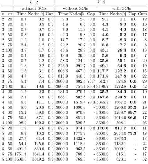
Table 1: Results obtained on the small dataset when solving the MILP formulation fork= 2 (without SCIs) and fork= 3 (with and without SCIs). Fork= 3 and for each instance, if both variants achieve an optimal solution, the smallest number of nodes and computing time are highlighted in boldface. If at least a variant does not achieve an optimal solution, the smallest gap is highlighted.

k=2 k=3

without SCIs without SCIs with SCIs

n m Time Nodes[k] Gap Time Nodes[k] Gap Time Nodes[k] Gap Cuts 2 20 0.1 0.2 0.0 2.3 2.0 0.0 2.1 1.1 0.0 12 2 30 0.7 0.5 0.0 4.8 6.5 0.0 4.3 5.0 0.0 10 2 40 0.7 0.7 0.0 7.9 11.3 0.0 4.1 4.0 0.0 18 2 50 0.8 0.6 0.0 9.3 9.8 0.0 4.0 5.2 0.0 17 2 60 1.2 1.0 0.0 14.7 17.9 0.0 8.7 8.3 0.0 8 2 75 2.4 1.2 0.0 20.2 20.7 0.0 8.8 7.7 0.0 8 2 100 3.8 1.7 0.0 43.6 28.9 0.0 43.1 28.4 0.0 13 3 20 0.4 0.9 0.0 13.9 29.0 0.0 5.6 9.3 0.0 7 3 30 0.7 1.2 0.0 58.3 124.4 0.0 35.6 55.1 0.0 20 3 40 1.8 2.2 0.0 226.9 291.7 0.0 49.1 64.6 0.0 19 3 50 1.5 3.1 0.0 603.6 467.0 0.0 117.7 122.2 0.0 15 3 60 4.7 5.1 0.0 615.9 440.3 0.0 171.5 147.8 0.0 22 3 75 5.4 7.4 0.0 3600.0 802.4 76.7 512.7 324.8 0.0 29 3 100 9.9 19.6 0.0 3600.0 757.1 89.4 3196.2 1272.8 0.0 42 4 20 1.2 2.3 0.0 131.0 270.1 0.0 35.2 84.0 0.0 10 4 30 2.1 3.8 0.0 633.1 802.8 0.0 167.8 224.8 0.0 11 4 40 5.6 11.1 0.0 3600.0 1519.4 79.3 3345.2 1867.2 0.0 21 4 50 8.6 20.8 0.0 3600.0 1096.8 - 3600.0 1206.085.3 19 4 60 15.2 39.0 0.0 3600.0 970.8 - 3600.0 1238.789.7 22 4 75 50.3 87.1 0.0 3600.0 851.1 - 3600.0 1014.986.6 17 4 100 98.9 192.3 0.0 3600.0 529.5 - 3600.0 508.1 - 26 5 20 1.9 5.6 0.0 679.6 974.1 0.0 170.0 311.7 0.0 11 5 30 6.3 16.2 0.0 3600.0 1775.3 - 3600.0 2054.073.3 18 5 40 27.7 61.4 0.0 3600.0 1422.8 - 3600.0 1363.3 - 13 5 50 54.4 125.6 0.0 3600.0 1118.3 - 3600.0 1132.1 - 24 5 60 491.2 830.6 0.0 3600.0 963.5 - 3600.0 1009.1 - 17 5 75 1751.1 1841.4 0.0 3600.0 788.0 - 3600.0 815.1 - 17 5 100 3600.0 3649.2 9.3 3600.0 769.3 - 3600.0 623.1 - 32

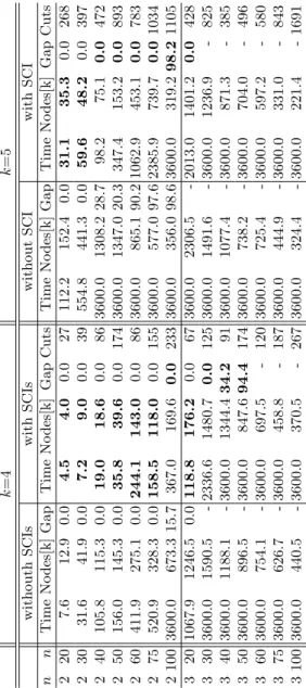
Table 2: Results obtained on the small dataset when solving the MILP formulation fork= 4,5 with and without SCIs. For each instance, if both variants achieve an optimal solution, the smallest number of nodes and computing time are highlighted in boldface. If at least a variant does not achieve an optimal solution, the smallest gap is highlighted.

k =4 k =5 withouth SCIs with SCIs without SCI with SCI n n Time No des[k] Gap Time No des[k] Gap Cuts Time No des[k] Gap Time No des[k] Gap Cuts 2 20 7.6 12.9 0.0 4.5 4.0 0.0 27 112.2 152.4 0.0 31.1 35 .3 0.0 268 2 30 31.6 41.9 0.0 7.2 9.0 0.0 39 554.8 441.3 0.0 59.6 48 .2 0.0 397 2 40 105.8 115.3 0.0 19.0 18.6 0.0 86 3600.0 1308.2 28.7 98.2 75.1 0.0 472 2 50 156.0 145.3 0.0 35.8 39.6 0.0 174 3600.0 1347.0 20.3 347.4 153.2 0.0 893 2 60 411.9 275.1 0.0 244.1 143.0 0.0 86 3600.0 865.1 90.2 1062.9 453.1 0.0 783 2 75 520.9 328.3 0.0 158.5 118.0 0.0 155 3600.0 577.0 97.6 2385.9 739.7 0.0 1034 2 100 3600.0 673.3 15.7 367.0 169.6 0.0 233 3600.0 356.0 98.6 3600.0 319.2 98.2 1105 3 20 1067.9 1246.5 0.0 118.8 176.2 0.0 67 3600.0 2306.5 -2013.0 1401.2 0.0 428 3 30 3600.0 1590.5 -2336.6 1480.7 0.0 125 3600.0 1491.6 -3600.0 1236.9 -825 3 40 3600.0 1188.1 -3600.0 1344.4 34.2 91 3600.0 1077.4 -3600.0 871.3 -385 3 50 3600.0 896.5 -3600.0 847.6 94.4 174 3600.0 738.2 -3600.0 704.0 -496 3 60 3600.0 754.1 -3600.0 697.5 -120 3600.0 725.4 -3600.0 597.2 -580 3 75 3600.0 626.7 -3600.0 458.8 -187 3600.0 444.9 -3600.0 331.0 -843 3 100 3600.0 440.5 -3600.0 370.5 -267 3600.0 324.4 -3600.0 221.4 -1691

The results are reported in Table 1 fork= 2,3 and in Table 2 for k= 4,5. In the second table, we omit the results for the instances withn= 4,5 as, both with or without SCIs, no solutions with a finite gap are found within the time

limit (i.e., the lower boundLB is always 0). Note that, fork= 2, symmetry is

broken by just fixing the top left element of the matrixX to 1, i.e., by letting, w.l.o.g.,x11= 1. Hence, we do not resort to the generation of SCIs in this case.

It has recently been argued that, in a number of data mining problems, feed-ing a heuristically generated solution to the MILP solver as a warm-start might give a significant performance boost [BM14]. Unfortunately, when

experiment-ing with this approach onk-PAMF-PLS, we only observed a negligible impact.

This is arguably due to the fact that, for hard instances, most of the difficulty in proving optimality lies in improving the dual bound, and running a heuristic (to obtain a primal bound) beforehand only incurs a overhead. For this reason, we have not used this approach in our experiments.

Let us neglect the case ofk= 2 and focus on the full set of 56k-PAMF-PLS

problems that are considered for this dataset (28 instances fork= 3 and 14 for

k= 4,5). Without SCI inequalities, we achieve an optimal solution in 24 cases

out of 56 (43%). The introduction of SCIs has a very positive impact. They allow to solve to optimality 10 more instances, for a total of 34 (60.1%). SCIs also yield a substantial reduction in both computing time and number of nodes. When focusing on the 24 instances solved by both variants of the algorithm, the overall results show that the introduction of SCIs yields a speedup, on (geometric) average, of almost 3 times, corresponding to a reduction of 66% of the computing times. The number of nodes is reduced by the same factor of 66%. Interestingly, this improvement is obtained by adding a rather small number of cuts which, in practice, prove to be highly effective. See, e.g., the

instance withm= 40, n= 3 which, when solved fork= 3 with SCIs, presents

a speedup in the computing time, when compared to the case without SCIs, of 4.6 times (corresponding to a reduction of 78%) with the sole introduction of 19 symmetry breaking constraints.

In our preliminary experiments, we observed the generation of a higher num-ber of cuts when employing older versions of CPLEX, such as 12.1 and 12.2 whereas, with CPLEX 12.5, their number is significantly smaller. This is, most likely, a consequence of the introduction of more aggressive techniques for sym-metry detection and symsym-metry breaking in the latest versions of CPLEX. We nevertheless remark that the improvement in computing time provided by the introduction of SCIs appears to be comparable for all the tested versions of CPLEX 12, regardless of the number of cuts that are generated.

Although the introduction of SCIs clearly increases the number of instances which can be solved to optimality, the results in Tables 1 and 2 show that the exact approach via mixed-integer linear programming might require large

computing times even for fairly small instances with n _≥ 3 and m _≥ 40 for

k _≥ 4. For k = 2, all the instances are solved to optimality, with the sole

exception of the instance with m= 100, n= 5 (on which we register a gap of

9.3%). Fork= 3, Table 1 shows that, already for n= 4 and m_≥50, the gap

becomes impractical forn= 3 andm_≥40 fork= 4, and forn= 3 andm_≥30 fork= 5.

6.4. Comparison between the four-step heuristic 4S-CR and the MILP formu-lation

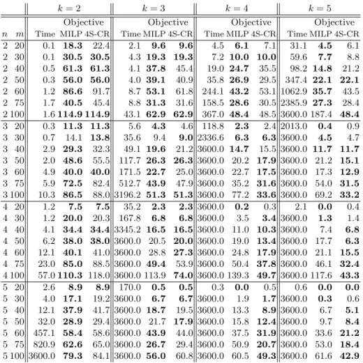
Before assessing the effectiveness of 4S-CR on larger instances, we compare the solutions it provides with the best ones found via mixed-integer linear pro-gramming on the small dataset (within the time limit). The results are reported in Table 3. For a fair comparison, 4S-CR is run, for the instances that are solved to optimality by the exact method, for the same time taken by the latter. For the instances for which an optimal solution has not been found, 4S-CR is run up to the time limit of 3600 seconds.

When comparing the quality of the solutions found by 4S-CR with those

found by the MILP formulation with SCIs, we register, fork= 2, very close to

optimal solutions with, on (geometric) average, a 4% larger fitting error. This

number decreases to 1% fork = 3. For larger values of k, namely k = 4 and

k= 5, for which the number of instances that are unsolved when adopting the

MILP formulation is much larger, 4S-CR yields solutions that are much better than those found via mixed-integer linear programming. When neglecting the instances with an optimal solution of value 0 (which would skew the geometric mean), the solutions provided by 4S-CR are, on geometric average, better than

those obtained via the exact method by 14% fork= 4 and by 20% fork= 5.

Fork = 2,3,4,5, 4S-CR finds equivalent or better solutions that those ob-tained via mixed-integer linear programming in, respectively, 11, 15, 18, and 19 cases, with strictly better solutions in, respectively, 1, 5, 16, and 15 cases. Overall, when considering the instances jointly, 4S-CR performs as good or bet-ter than mixed-integer linear programming in 63 cases out of 112 (28 instances, each solved 4 times, once per value ofk), strictly improving over the latter in 37 cases. This indicates that the quality of the solutions found via 4S-CR can be quite high even for small-size instances and that the difference w.r.t. the exact method, at least on the instances for which a comparison is viable, seems to be

increasing with the number of pointsm, the number of dimensionsn, and the

number of submodelsk.

Note that, for the instance withm= 30, n= 3 and for bothk= 2 andk= 3,

the MILP formulation yields, in strictly less than the time limit, a solution which is worse than the corresponding one found by 4S-CR. As discussed in Section 4, this is most likely due to the selection of too small values for the parameters

M1 and M2. Experimentally, we observed that the issue can be avoided by

choosingM =M1=M2= 10000, although at the cost of a substantially larger

computing time (due to the need for a higher numerical precision to handle the larger differences between the magnitudes of the coefficients in the formulation). 6.5. Experiments with 4S-CR and some variants

We now present and discuss the results obtained with 4S-CR and some variants on larger instances, and assess the impact of the main features of 4S-CR (i.e., the criterion for identifying and reassigning critical points in thePoint

Table 3: Comparison between the best results obtained fork= 2,3,4,5 on the small instances when solving the MILP formulation (with symmetry breaking constraints and within a time limit of 3600 seconds) and those obtained via 4S-CR. The latter is run for as much time as that required to solve the MILP formulation (within the time limit). For each instance, the value of the best solution found is highlighted in boldface.

k= 2 k= 3 k= 4 k= 5

Objective Objective Objective Objective

n m Time MILP 4S-CR Time MILP 4S-CR Time MILP 4S-CR Time MILP 4S-CR 2 20 0.1 18.3 22.4 2.1 9.6 9.6 4.5 6.1 7.1 31.1 4.5 6.1 2 30 0.1 30.5 30.5 4.3 19.3 19.3 7.2 10.0 10.0 59.6 7.7 8.8 2 40 0.5 61.3 61.3 4.1 37.8 45.4 19.0 24.7 35.5 98.2 14.8 21.2 2 50 0.3 56.0 56.0 4.0 39.1 40.9 35.8 26.9 29.5 347.4 22.1 22.1 2 60 1.2 86.6 91.7 8.7 53.1 61.8 244.1 43.2 53.1 1062.9 35.7 43.5 2 75 1.7 40.5 45.4 8.8 31.3 31.6 158.5 28.6 30.5 2385.9 27.3 28.4 2 100 1.6114.9 114.9 43.1 62.9 62.9 367.0 48.4 48.5 3600.0 187.4 48.4 3 20 0.3 11.3 11.3 5.6 4.3 4.6 118.8 2.3 2.4 2013.0 0.4 0.9 3 30 0.7 14.1 13.8 35.6 9.4 9.0 2336.6 6.3 6.3 3600.0 4.5 4.7 3 40 2.9 29.3 32.3 49.1 19.6 21.2 3600.0 14.7 15.5 3600.0 11.7 11.7 3 50 2.0 48.6 55.5 117.7 26.3 26.3 3600.0 20.2 17.9 3600.0 21.2 15.1 3 60 4.9 40.0 40.0 171.5 22.7 25.0 3600.0 22.7 17.5 3600.0 17.3 12.9 3 75 5.9 72.5 82.4 512.7 43.9 47.9 3600.0 35.2 31.6 3600.0 54.0 31.5 3 100 10.3 86.5 88.0 3196.2 51.3 51.3 3600.0 77.2 33.6 3600.0 69.2 33.2 4 20 1.2 7.5 7.5 35.2 2.3 2.3 3600.0 0.2 0.3 2.1 0.0 0.4 4 30 1.2 20.0 20.3 167.8 6.8 6.8 3600.0 3.5 3.4 3600.0 1.3 1.4 4 40 4.1 34.4 34.43345.2 16.5 16.5 3600.0 11.0 10.3 3600.0 7.4 6.8 4 50 6.2 38.0 38.03600.0 20.5 20.0 3600.0 19.0 13.4 3600.0 17.7 6.3 4 60 12.1 40.1 41.0 3600.0 28.8 27.3 3600.0 24.8 17.9 3600.0 21.1 15.5 4 75 23.0 85.0 88.5 3600.0 49.4 53.9 3600.0 50.4 37.8 3600.0 46.1 32.4 4 100 57.0110.3 118.0 3600.0 113.9 74.0 3600.0 139.3 49.7 3600.0 117.6 43.3 5 20 2.6 8.9 8.9 170.0 0.5 0.5 0.3 0.0 0.5 0.6 0.0 0.0 5 30 4.0 17.1 19.2 3600.0 6.7 6.7 3600.0 1.9 1.7 3600.0 0.3 0.6 5 40 12.1 37.9 41.7 3600.0 18.7 19.5 3600.0 13.3 8.9 3600.0 6.7 5.1 5 50 32.0 28.9 29.4 3600.0 21.7 17.9 3600.0 15.8 12.4 3600.0 9.7 8.4 5 60 457.1 58.4 58.6 3600.0 43.9 44.0 3600.0 37.5 31.9 3600.0 33.6 21.2 5 75 820.9 62.6 65.0 3600.0 26.7 29.4 3600.0 50.9 20.7 3600.0 53.0 18.4 5 100 3600.0 79.3 84.1 3600.0 56.0 60.8 3600.0 60.5 49.3 3600.0 61.6 42.9

Partitionstep, theDomain Partitionstep, and thePartition Consistency

step, applied at each iteration) on the quality of the solutions found.

As already mentioned, we set ρ= 0.5 in all the experiments involving our

criterion for identifying critical points and we consider a tabu list with a memory of two iterations. When tuning the parameters, we observed improved results on

the smaller instances when increasingρ, as opposed to worse ones on the larger

instances. This is, most likely, a consequence of the number of iterations carried

out within the time limit, which becomes much smaller for a larger value ofρ,

thus forcing the method to halt with a solution which is too close to the start-ing one. As to the tabu list, we observed that a short memory of two iterations suffices to prevent loops. Indeed, due to the nature of the problem as well as

due to the many aspects ofk-PAMF-PLS that our method considers, the values

of the parameters of the piecewise affine submodels change often dramatically within very few iterations. This way, few iterations taking place after a wors-ening move typically suffice to prevent that a point-to-submodel reassignment could take place twice, thus making the occurrence of loops extremely unlikely.

To assess the impact of the Point Partition step based on the criterion

for critical points (and on the corresponding control parameter), we introduce a variant of 4S-CR where, in the former step,every point (ai, bi) is (re)assigned

to a submodel yielding the smallest fitting error. This is in line with the reas-signment step of many popular clustering heuristics, as reported in Sections 2 and 5. We refer to this method as 4S-CL (where “CL” stands for “closest”).

To evaluate the relevance of considering, in 4S-CR, the domain partition

aspect directly at each iteration (via the Domain Partition and Partition

Consistency steps), as well as to compare 4S-CR to classical algorithms, we

also consider a standard (STD) two-phase method which, first, addresses the

clustering aspect ofk-PAMF-PLS and, only at the end, before halting, takes the

domain partition aspect into account, thus tackling the problem in two distinct, successive phases: a clustering phase and a classification phase. In the algo-rithm, which we consider in two versions, we iteratively alternate between the

Submodel FittingandPoint Partitionsteps. In thePoint Partitionstep,

we either reassign every point to the “closest” submodel (STD-CL) or to that indicated by our criterion (STD-CR). After a local minimum has been reached, a piecewise linearly separable domain partition with minimum misclassification error is derived by solving only once a multicategory linear classification prob-lem via linear programming, as in Probprob-lem (25)–(28). Since STD-CL is similar to most of the standard techniques proposed in the literature, we consider it as the baseline method and compare the other methods (4S-CR, 4S-CL, and STD-CR) to it.

For the sake of comparison, we also consider an extension of this standard method, STD-CL, obtained after introducing an extra third phase, based on the refinement point-reassignment criterion proposed in [BGPV05], taking place between the clustering and classification phases. We refer to this algorithm as STD-CL-B. This refinement criterion is based on the identification of so-called

undecidablepoints, namely, data points which lie within a maximum given error

undecidable data point ai is iteratively reassigned to the submodel to which

the majority of the c points which are closer, in `2-norm, to ai are currently

assigned. We remark that [BGPV05] addresses a piecewise-affine model fitting

problem where k is minimized, subject to a maximum fitting error of δ. To

adapt the criterion tok-PAMF-PLS, we set, in our experiments,δto the average

fitting error between each data point and its current submodel. As suggested

in [BGPV05], we select c= 10 and carry out the reassignment of undecidable

points 5 times, each time followed by aSubmodel Fittingstep7.

The results for the medium, large, and UCI datasets, obtained within a time limit of, respectively, 900, 1800, and 900 seconds, are reported in Table 4. The comparison shows that 4S-CR outperforms the baseline method STD-CL in almost all the cases. When considering the medium instances, 4S-CR yields an improvement in objective function value of, on geometric average, 8%, 21%,

21%, and 24% for, respectively,k= 2, 3, 4, and 5. On the large instances, the

improvement is of 16%, 24%, 29%, and 24%. For the four UCI instances, the improvement is of 6%, 9%, 13%, and 16%. When considering the three datasets jointly, the improvement is of 8%, 21%, 21%, 24%. On geometric average, for

all the values ofk, 4S-CR improves on the fitting error of STD-CL by 20%. On

a total of 112 instances (for the different values ofk) ofk-PAMF-PLS, 4S-CR

achieves the best solution in 103 cases (92%).

When comparing 4S-CL to STD-CL, we register, on geometric mean and

for the different values ofk, an improvement of 4%, 9%, 10%, and 16% on the

medium instances, of 12%, 17%, 17%, and 11% on the large ones, and of 4%, 9%, 10%, and 16% on the UCI datasets. When considering all the datasets and all the values ofkjointly, the improvement is of 12%. Although still substantial, this value is not as large as that for 4S-CR, thus highlighting the relevance of our

criterion based on critical points which is adopted in thePoint Partitionstep.

At the same time, it also shows that, even without the criterion, the central idea of 4S-CR (i.e., considering the domain partition aspect of the problem directly at each iteration, rather than deferring it to a final phase) has a large positive impact on the solution quality.

Most interestingly, the results for STD-CR are quite poor. When

consid-ering all the 112 instances (for the different values of k), the method yields,

on geometric average, a 4% larger fitting error w.r.t. STD-CL. This is not surprising as, by constructing a domain partition only at the very end of the algorithm, the solutions that are obtained before its derivation typically contain a large number of misclassified points, which yield a large negative contribution to the final fitting error. Indeed, when comparing the value of the solutions that are found before and after carrying out the domain partition phase at the end of the method, we register an increase in fitting error of up to 4 times for

7_{Experiments with δ equal to the average fitting error scaled by a factor of} {0.1,0.25,0.50,0.75,1} revealed that the best results are obtained with a factor of 1. We also experimented withc= 5,20,50 and carrying out 1, 10, and 20 passes of the criterion. On average, on average, we obtained comparable results.

Table 4: Results obtained with 4S-CR, when compared to STD-CL, STD-CR, 4S-CL, and STD-CL-B on the medium, large, and UCI instances, within a time limit of, respectively, 900, 1800, and 900 seconds, fork = 2,3,4,5. For each instance, the value of the best solution found is highlighted in boldface.

k = 2 k = 3 k = 4 k=5 n m STD-4S-CL 4S-CR STD-4S-CL 4S-CR STD-4S-CL 4S-CR STD-4S-CL 4S-CR STD-CL CR CL-B CL CR CL-B CL CR CL-B CL CR CL-B 2 500 658.6 863.4 659.7 592.7 658.7 660.2 734.7 592.7 472.9 660.2 638.3 790.6 485.8 345.7 610.8 638.3 784.9 493.1 472.9 663.4 2 500 406.2 406.2 406.2 406.2 406.2 400.1 400.1 400.1 274.1 400.1 416.8 416.8 387.8 254.0 416.8 416.8 400.1 383.6 254.0 416.8 2 500 408.5 408.5 408.4 408.4 408.5 365.6 292.7 394.3 267.4 408.6 288.7 265.4 325.6 266.7 281 .0 330.5 424.4 325.6 226.3 329.1 3 500 392.1 386.7 378.7 358.2 391.8 334.0 346.1 310.7 279.2 334.6 318.6 319.9 309.9 286.6 329.8 345.5 351.0 310.5 281.3 288.4 3 500 518.3 484.1 472.9 448.5 506.8 500.3 371.6 300.0 262.7 501.3 496.2 511.8 288.2 257.4 494.9 491.3 533.3 292.4 256.8 408.1 3 500 699.7 698.6 580.4 574.6 750.0 612.2 627.9 508.8 447.1 522.9 502.1 548.1 447.9 449.3 459.0 532.7 564.3 411.1 427.6 503.0 4 500 421.1 426.6 412.2 403.7 424.6 378.0 392.0 334.1 325.3 360.3 308.4 325.2 268.8 260.2 295.8 328.1 339.1 206.2 193.0 234.0 4 500 669.0 670.0 643.0 623.8 668.5 536.6 521.1 505.5 474.3 546.2 435.5 492.3 395.7 375.2 394.8 423.4 429.2 377.2 318.8 339.4 4 500 642.2 625.2 587.0 569.3 641.6 553.9 516.2 528.5 513.2 597.5 550.9 580.9 474.9 493.1 539.9 566.9 566.9 479.5 472.4 534.2 5 500 531.7 511.6 520.5 503.9 531.7 381.8 403.2 370.4 360.8 368.5 280.4 348.2 264.0 242.8 288.9 277.6 278.7 230.3 264.7 288.7 5 500 373.9 399.0 371.4 344.9 384.4 257.3 388.7 261.0 252.3 257.3 246.1 273.9 240.7 230.5 241.8 232.0 298.9 237.7 218.8 233.8 5 500 635.1 616.0 603.4 593.7 626.1 610.4 592.0 536.4 509.8 605.9 449.3 616.0 472.5 421.7 456.6 441.4 620.6 464.5 489.0 426.0 2 1000 654.5 654.5 654.5 654.5 654.5 654.1 654.1 572.5 572.5 654.1 654.6 670.0 572.5 557.6 654.6 565.7 644.5 572.5 557.8 565.7 2 1000 1685.4 1618.5 1452.5 1241.9 1685.4 1685.4 916.0 931.0 790.5 1685.4 1715.6 1994.0 931.0 581.6 1918.1 1208.2 1903.3 931.0 647.8 1504.8 2 1000 1423.0 1042.1 1019.9 953.2 1423.0 1102.5 970.6 849.1 634.3 1124.7 1190.9 1405.6 809.0 501.1 1195.7 953.2 1289.1 752.0 490.1 1233.1 3 1000 1371.2 1127.6 1095.8 976.8 1397.5 1182.8 1053.2 743.2 729.7 1196.6 780.3 1089.1 732.0 621.9 1041.5 1003.7 1132.4 714.2 605.7 1075.6 3 1000 1099.5 1072.9 1023.5 935.8 1099.5 969.5 1010.8 953.6 829.5 974.8 997.3 1014.7 934.8 793.6 1022.0 957.3 1047.9 943.4 654.5 1033.6 3 1000 1545.1 1408.3 1107.6 1084.2 1545.1 1217.2 1171.3 853.9 805.0 1172.7 1152.5 1209.7 777.9 536.4 1145.5 919.5 1258.6 777.9 616.5 993.0 4 1000 520.1 516.2 519.4 503.9 520.1 520.1 547.7 481.1 422.3 520.1 520.1 557.3 438.2 455.0 537.7 503.7 514.3 483.1 443.1 536.1 4 1000 672.8 672.6 666.0 655.0 672.8 536.9 544.7 502.9 480.8 518.6 500.7 513.8 481.9 450.9 484.4 511.2 521.9 478.5 463.6 484.3 4 1000 1154.7 1076.1 951.0 924.1 1154.7 963.3 979.4 854.6 797.7 984.5 869.5 895.1 705.8 625.1 765.3 928.0 950.6 758.5 710.4 794.2 5 1000 1174.6 1165.9 1110.6 1092.8 1185.5 1079.3 1061.9 972.2 941.1 1073.8 910.1 883.1 861.4 846.0 868.6 915.8 1049.4 880.2 856.1 793.9 5 1000 985.3 936.9 878.6 859.3 994.5 760.3 912.1 704.9 685.8 785.1 671.9 689.2 641.4 614.7 654.5 671.2 717.1 656.9 646.8 631.8 5 1000 570.3 568.1 573.2 565.2 579.2 487.7 531.5 491.3 471.5 488.2 474.0 521.2 469.9 464.5 481.6 481.4 486.5 476.2 451.3 481.2 3 397 23.0 23.0 22.6 22.1 23.8 21.2 23.9 21.0 20.8 21.5 21.2 23.9 19.5 19.7 21.9 21.0 23.3 18.2 19.1 21.6 5 698 40.0 35.7 40.0 35.7 40.0 35.7 33.6 35.7 33.6 36.1 35.7 33.6 35.7 31.5 35.7 35.7 33.6 33.6 31.5 35.7 5 209 28.0 28.2 27.6 27.0 27.9 25.2 27.5 23.4 22.2 25.8 24.4 29.2 21.6 20.7 26.2 25.9 29.2 21.0 20.1 25.5 8 506 142.6 145.9 135.5 134.9 142.1 132.8 146.6 114.6 112.4 134.1 131.1 150.1 110.0 107.0 135.5 135.4 134.5 103.8 106.7 135.4 25