A MapReduce Solution for Associative Classification of
Big Data
Alessio Bechini, Francesco Marcelloni∗, Armando Segatori Dipartimento di Ingegneria dell’Informazione
University of Pisa 56122, Pisa, Italy
Abstract
Associative classifiers have proven to be very effective in classification prob-lems. Unfortunately, the algorithms used for learning these classifiers are not able to satisfactorily manage big data because of time complexity and memory constraints. To overcome such drawbacks, we propose a distributed association rule-based classification scheme shaped according to the MapRe-duce paradigm. The scheme mines classification association rules (CARs) using a distributed version of the well-known FP-Growth algorithm. Once CARs have been mined, a distributed pruning based on dataset coverage is applied. The set of survived CARs are used to classify unlabeled patterns.
The memory usage and time complexity for each phase of the learning process are discussed, and the scheme is evaluated on three real-world big datasets on the Hadoop framework, characterizing its scalability and the achievable speedup on small computer clusters. The proposed solution for associative classifiers turns to be suitable to practically address big datasets
∗Corresponding Author: Tel: +39 050 2217678 Fax: +39 050 2217600 Email address: [email protected](Francesco Marcelloni)
even with modest hardware support.
Keywords: Associative Classifiers; Big Data; Hadoop; MapReduce; Parallel FP-Growth
1. Introduction
Classifiers based on association relationships, generally known as Asso-ciative Classifiers (ACs), integrate two well-known data mining paradigms: pattern classification and association rule mining [1]. Pattern classification assigns a class label to an object described by a set of features using a specific model, namely the classifier, previously built by exploiting a set of training examples. Association rule mining is the task of discovering correlation or other relationships among items in large databases [2]. Several different works [3, 4, 5, 6, 7, 8] have shown that ACs achieve high classification perfor-mances and are more accurate than traditional algorithms such as C4.5 [9]. Furthermore, since associative relationships reflect the close dependencies among predictive variables, the extraction of highly confident rules produces rule-based models more interpretable than models generated by using other techniques [10, 11]. Thus, in the last years, ACs have been successfully ex-ploited in a number of real world applications such as phishing detection in websites [12], XML document classification [13], text analysis [14], and disease classification [14, 15].
Generally, an AC operates in three phases. In the first phase, a set of classification association rules (CARs) is mined from the training set. Preliminarily, the attribute values (items in the association rule context) characterized by an occurrence value beyond a given threshold, calledfrequent
items, are selected from the dataset. Then, CARs are mined from frequent items. In the second phase, CARs are pruned according to support and confidence thresholds, and redundancy. Finally, the selected CARs are used to predict the class labels on input unlabeled patterns.
To mine CARs two algorithms are typically used: the Apriori algorithm [2] and the frequent pattern growth [16], or simply FP-Growth algorithm.
The Apriori algorithm generates candidate itemsets by extending frequent itemsets one item at a time, and then tests their frequency against the over-all dataset. When no further successful frequent extensions can be mined, the algorithm terminates. In many cases this “bottom up” approach leads to a good performance gain, especially when the candidate generate-and-test steps significantly reduce the size of candidate sets. However, the Apriori algorithm repeatedly scans the overall dataset for evaluating whether can-didate itemsets are frequent. This scanning process can be very expensive, especially with very large datasets that cannot be stored in the main memory [17].
FP-Growth mines the complete set of frequent itemsets without generat-ing all the possible candidate itemsets, by scanngenerat-ing the overall dataset only twice. First, it extracts the frequent items and sorts them by descending fre-quencies. Then, the dataset consisting only of frequent items is compressed into a frequent pattern tree, called FP-tree. Finally, FP-Growth recursively mines patterns by dividing the compressed dataset into a set of projected datasets, each associated with a frequent item or a pattern fragment. For each pattern fragment, only its associated conditional dataset needs to be ex-amined. The problem of mining frequent itemsets is converted into building
and searching trees recursively.
The different approaches proposed in the literature to generate ACs aim to improve classification accuracy and often neglect to consider the time and space requirements [11] needed for generating CARs. Nowadays, when deal-ing with big data, that is, datasets whose size is beyond the ability of typical database software tools to capture, store, manage and analyze, most of the classification learning algorithms proposed in the literature are practically inapplicable [18]. On the other hand, when the numbers of features and/or data objects grow up, the number of fake correlations also increments [19].
A simple solution to deal with massive data is to select only a subset of data objects so that the traditional data mining algorithms can be executed in a reasonable time. However, downsampling techniques may delete useful knowledge. Thus, approaches that consider the overall dataset are more de-sirable. In the last years, different scalable and parallel implementations have been proposed for association rule mining. Most of these implementations have focused on the well-known FP-Growth algorithm. Since the FP-Growth algorithm requires just two scans of the dataset, it is computationally more efficient than the Apriori algorithm. Some works have proposed to parallelize the FP-Growth algorithm exploiting multiple threads on a shared memory environment [20, 21]. In [22], a distributed version, which takes both data and computation across multiple machines into account, has been proposed. Other works investigate different parallel implementations, addressing some issues such as communication cost, data placement strategies, memory and I/O utilization [23]. All these approaches are based on the MPI (Message Passing Interface) programming model [24] and achieve good performance in
terms of scalability and speedup. However, these approaches are limited by memory bottlenecks and communication overheads.
Recently, the MapReduce programming paradigm has become one of the most popular models to deal with Big Data. Originally proposed by Google in 2004 [25], the paradigm simplifies the parallelization of the computation flow across large-scale clusters of machines. Further, MapReduce execution environments, like e.g. Apache Hadoop [26], take care of failures and com-munications among different cluster machines [25, 27]. Some recent works have proposed several parallel MapReduce solutions of classical data min-ing algorithms, such as k-means [28], SVM [29, 30, 31], KNN [32], frequent pattern mining [18, 33, 34], boosting [35], nayve Bayes, neural network back-propagation, and logistic regression, investigating performance in terms of speedup [36]. To the best of our knowledge, however, no paper has discussed the implementation of associative classifiers on MapReduce.
In this paper, we propose an association rule-based classification scheme built upon the MapReduce framework. The proposed scheme mines CARs using a distributed version of the FP-Growth algorithm. Once CARs have been mined, a distributed pruning based on the dataset coverage threshold proposed in [4] is applied. The set of survived rules are used to classify unlabeled patterns. We discuss memory usage and time complexity for each phase of the learning process.
We performed two different experiments. In the first experiment, we used 18 ordinary-sized benchmarks to show that our scheme achieves accuracies comparable to other three well-known associative classifiers, namely CBA, CBA2 and CPAR. In the second experiment, we adopted three real-world big
datasets with different numbers of instances (up to 11 millions) to analyze scalability and speedup of each parallel job according to different units of work and problem size.
The paper is organized as follows. Section 2 provides some preliminaries on ACs and MapReduce. Section 3 describes the proposed approach and includes the details of each single job that runs on the cluster of machines. Section 4 presents the experimental setup and discusses the results in terms of accuracy, speedup and scalability. Finally, in Section 5, we draw final conclusions.
2. Background
2.1. Associative Classifiers
Pattern classification consists of assigning a class Cl from a predefined set C = {C1, . . . , CL} of classes to an unlabeled pattern. We consider a pattern as an F-dimensional vector of features. Let X = {X1, . . . , XF} be the set of the F features and Uf, f = 1, . . . , F, be the universe of the fth feature. Features can be both continuous and categorical. Continuous features are discretized, that is, their universes are partitioned into con-tiguous intervals before performing the association rule mining process. Let Ps={[as,1, as,2],(as,2, as,3], . . . ,(as,Ts, as,Ts+1]}be a partition of Ts contiguous
intervals on the continuous featureXs. Since each interval can be associated with a label, continuous features can be managed as categorical features. Let Vf = {vf,1, . . . , vf,Tf} be the set of values associated with feature Xf,
f = 1, . . . , F. In case of continuous features, each label vf,j, withj ∈[1..Tf], identifies the jth interval [af,j, af,j+1] of the partition of Xf.
Association rules are rules in the form Z → Y, where Z and Y are sets of items. These rules describe relations among items in a dataset [17]. Association rules have been widely employed in the market basket analysis. Here, items identify products and the rules describe dependencies among the different products bought by customers [2]. Such relations can be used for decisions about marketing activities as promotional pricing or product placements.
In the associative classification context, the single item is defined as the couple If,j = (Xf, vf,j), where vf,j is one of the values that the variable Xf, f = 1, ..., F, can assume. A generic classification association rule CARm is expressed as:
CARm :Antm →Clm (1)
where Antm is a conjunction of items, and Clm is the class label selected
for the rule within the set C = {C1, . . . , CL} of possible classes. For each variableXf, just one item is typically considered inAntm. AntecedentAntm can be represented more friendly as
Antm :X1 isv1,jm,1 . . . AND . . . XF isvF,jm,F (2)
where vf,jm,f is the value used for variable Xf in rule CARm.
LetT = (x1, y1),(x2, y2), . . . ,(xN, yN) be the training set, where, for each object (xi, yi), xi,f, i = 1, . . . , N, is one of the discrete values that feature Xf,f = 1, . . . , F, can assume and yi ∈C. In case of continuous features, we replace the real value with the corresponding categorical value, that is, the value associated with the interval which the real value belongs to. We state
that xi matches a ruleCARm if and only if, for each item If,j inAntm with f = 1, . . . , F, the value xi,f of xi has the same value vf,jm,f of item If,j for
the feature Xf in the rule.
In the association rule analysis, support and confidence are the most common measures to determine the strength of an association rule. Support of a classification association rule CARm, in short supp(Antm → Clm), is
the number of objects in the training set T matching antecedent Antm and having Clm as class label. Usually, the support value is normalized with the
total number of objects. Support can be interpreted as the coverage of rule CARm in T and estimates the number of instances correctly classified by rule CARm.
Confidence of CARm, in short conf(Antm → Clm), is the ratio between
supp(Antm → Clm) and the number of objects in T matching antecedent
Antm. The value can be interpreted as the probability of correctly classifying the class label Clm in the unlabeled pattern bx under the condition that xb
matches Antm. Formally, support and confidence can be expressed for a classification association rule CARm as follows:
supp(Antm →Clm) = supp(Antm∪Clm) N (3) conf(Antm →Clm) = supp(Antm∪Clm) supp(Antm) (4) where N is the number of objects in T, supp(Antm ∪Clm) is the number
of objects in T matching pattern Antm and having Clm as class label and
supp(Antm) is the number of objects in T matching pattern Antm.
An AC is also characterized by its reasoning method, which uses the in-formation from the rule base to determine the class label for a specific input
pattern. In our AC scheme, we use the weighted χ2 reasoning method as
described in Section 3.4. 2.2. MapReduce
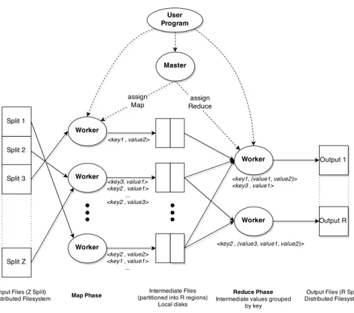
In 2004, Google proposed the MapReduce programming framework [25]. The framework divides the work into a set of independent tasks and paral-lelizes the computation flow across large-scale clusters of machines, taking care of communications among them and possible failures, and efficiently handling network bandwidth and disk usage. MapReduce is a programming model based on functional programming, designed for processing large vol-umes of data with parallel and distributed algorithms on a computer cluster. It divides the computational flow into two main phases: Map and Reduce. By simply designing Map and Reduce functions, developers are able to de-velop parallel algorithms that can be executed across the cluster. The overall computation is organized around hkey, valuei pairs: it takes a set of input
hkey, valuei pairs and produces a set of output hkey, valuei pairs. Figure 1 shows the MapReduce flow.
When the MapReduce execution environment executes a user program, it automatically partitions the dataset into a set of Z independent splits that can be processed in parallel by different machines. While the number of map tasks is determined by the number Z of the input splits, the number R of reducers is defined by the user. Thus, there are Z map tasks and R reduce tasks which have to be executed. Furthermore, the MapReduce framework starts up many copies of the user program on the machine cluster. One copy is denoted as master: the master schedules and handles tasks within the cluster. The others are called workers. The master assigns a map task or a
reduce task to any idle worker. When a map task is assigned to a worker, the worker reads the contents of the corresponding input split, parses the
hkey, valuei pairs of the input data and passes the computational flow to the user-defined Map function. The Map function takes a singlehkey, valuei
pair as input and produces a list of intermediatehkey, valueipairs as output. This process can be represented as:
map(key1, value1)→list(key2, value2) (5) Workers periodically store in the local disk the intermediate values produced by map functions and partition these values into R regions. Each region represents the intermediate subspace of the key space and is generated by a partitioning function (for instancehash(key)modR). Finally, these workers return back results to the master that is responsible for notifying reduce workers. When a reduce worker is notified, it reads remote intermediate data from the local disks of map workers, and groups and sorts them according to the intermediate key. Then, it iterates over the sorted intermediate data and, for each unique key, passes the computational flow to the Reduce function defined by the user. The Reduce function takes the key and the associated value list as input and generates a new list of values as output. This process can be summarized as:
map(key2, list(value2))→list(value2) (6) Finally, the output of the reduce function is appended to the output final file.
In the last years, several open source projects have been developed to deal with big data, thanks also to the contribution offered by companies such as
Facebook, Yahoo! and Twitter. Some examples are: Spark [37], a fast and general engine for large-scale data processing, Apache S4 [38], a platform for processing continuous data streams, Storm [39], a software for streaming data-intensive distributed applications similar to S4, Dremel [40] and Apache Drill [41], scalable, interactive low latency ad hoc query systems for analysis of read-only nested data.
The most popular open source execution environment for the MapReduce paradigm is Apache Hadoop [26, 42]. It allows the execution of custom applications that rapidly process big datasets stored in its distributed file system, called Hadoop Distributed Filesystem (HDFS). On the top of Hadoop several related projects such as Apache Pig [43], Apache Hive [44], Apache HBase [45], Apache ZooKeeper [46] have been developed. As regards data mining tools for big data there are many initiatives. Mahout [47, 48] is the most popular open source machine learning library that runs on the top of Hadoop. It implements a wide range of machine learning and data mining algorithms for clustering, recommendation systems, classification problems and frequent pattern mining. Other tools are MOA [49], Vowpal Wabbit [50] and, for the Big Graph mining problem, PEGASUS [51] and GraphLab [52].
3. The MapReduce Associative Classifier
In Section 1 we have pointed out that the current implementations of associative classifiers are not able to manage big data. In this section, we describe our implementation of an associative classifier using the MapReduce paradigm on the Hadoop framework. The classifier is an extension of the well-known CMAR [4] algorithm in a distributed execution environment.
The MapReduce Associative Classifier (MRAC) consists of the following three steps:
1. Discretization: a partition is defined on each continuous feature by using the multi-interval discretization approach based on entropy pro-posed by Fayyad and Irani in [53]; this step is performed before starting the MapReduce execution.
2. CAR Mining: a MapReduce frequent pattern mining algorithm, which is an extension of the well known FP-Growth algorithm described in [18], is exploited to extract frequent CARs with support, confidence and chi-squared higher than pre-fixed thresholds;
3. Pruning: rule pruning based on redundancy and training set coverage is applied to generate the final rule base.
In the following, we discuss the three steps in detail. 3.1. Discretization
The discretization of continuous features is a critical aspect in AC gener-ation, and so far several different heuristic algorithms have been proposed to this aim [53, 54, 55, 56]. For MRAC we use the method proposed by Fayyad and Irani in [53]. This supervised method has been already adopted for dis-cretizing continuous features in CMAR and has proved to be very effective [4]. The method selects the boundaries of each bin by exploiting the class information entropy of candidate partitions.
LetTf,0 = [x1,f, ..., xN,f]T the projection of the training setT along vari-able Xf and af,r a cut point for the same variable. Let Tf,1 and Tf,2 be
by af,r. The class information entropy of the discretization induced by af,r, denoted as E(Xf, af,r;Tf,0) is given by E(Xf, af,r;Tf,0) = |Tf,1| |Tf,0| ·Ent(Tf,1) + |Tf,2| |Tf,0| ·Ent(Tf,2) (7)
where|| denotes the cardinality andEnt() is the entropy calculated for a set of points [53]. The cut point af,min, which minimizes the class information entropy over all possible binary partitions of Tf,0, is selected. The method is
then applied recursively to both the intervals induced byaf,minuntil the fol-lowing stopping criterion based on the Minimal Description Length Principle is achieved: Gain(Xf, af,min;Tf,0)< log2(|Tf,0| −1) |Tf,0| +∆(Xf, af,min;Tf,0) |Tf,0| (8) where
Gain(Xf, af,min;Tf,0) = Ent(Tf,0)−E(Xf, af,min;Tf,0), (9)
∆(Xf, af,min;Tf,0) = log2(3
k0−2)−[k
0·Ent(Tf,0)−k1·Ent(Tf,1)−k2·Ent(Tf,2)]
(10) and ki is the number of class labels represented in the set Tf,i.
The method outputs, for each feature, a set of cut points. Let Uf = [xf,l, xf,u] be the universe of variable Xf. Let {af,1, . . . , af,Tf+1}, with ∀r ∈
[1, . . . , Tf], af,r < af,r+1, be the set of cut points, where af,1 = xf,l and af,Tf+1 =xf,u. Then, the method identifies the set{[af,1, af,2], . . . ,
af,Tf, af,Tf+1
}
of contiguous intervals, which partition the universe of variableXf. If no cut point has been found by the algorithm for feature Xf, then no interval is generated for the feature: Xf is then discarded. We perform the discretiza-tion algorithm on a percentage of randomly extracted objects from the entire
training set. In the experiments on big datasets, we used 10% of the overall training set.
We associate each interval [af,r, af,r+1], r ∈ [1, . . . , Tf] with a categorical value vf,r. Each categorical value represents an item.
3.2. CAR Mining
To mine the CARs from the training set, we adopt the well known FP-Growth mining algorithm. Our MapReduce implementation is based on the Parallel FP-Growth (PFP-Growth) proposed by Li et al. [18] for efficiently parallelizing the frequent patterns mining without generating candidate item-sets. The PFP-Growth algorithm breaks down a large-scale mining task into independent, parallel tasks and uses three MapReduce phases to generate frequent patterns. The dataset is divided into parts (shards) and each part is stored on a different node. In the first phase, the algorithm counts the support values of all items that appear in dataset. Each mapper inputs one shard. In the second phase, each node builds a local and independent tree and recursively mines the frequent patterns from it. Such a subdivision requires the entire dataset to be projected onto different item-conditional datasets. An item-conditional dataset T(If,j), also called item-projected dataset, is a dataset restricted to the objects where the specific item If,j occurs. In each object of the T(If,j), named item-projected object, the items with lower sup-port than If,j are removed and the others are sorted according to the de-scending order of their support. Since the FP-Tree building processes are independent of each other, all the item-projected datasets can be distributed over the nodes and processed independently.
previous phase and, for each item, selects only the K highest supported patterns. As shown by empirical studies, the PFP-Growth algorithm achieves a near-linear speedup [18].
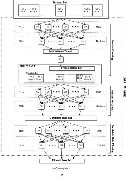
We adapted the PFP-Growth algorithm to generate high-confidence and frequent classification association rules. As shown in Figure 2, our algorithm also uses three MapReduce phases: Parallel Counting, Parallel FP-Growth and Candidate Rule Filtering.
The first MapReduce phase scans the dataset and counts the support values of each item. Each mapper analyzes an HDFS block: the input key-value pair is represented by hkey, value = oii, where oi is an object of the training set block. For each item vf,j ∈ oi, the mapper outputs a key-value pair hkey = vf,j, value = 1i. The reducer is fed by a list of corresponding values for each key (in this case a set of 1’s) that we call List(key) and out-puts hkey =vf,j, value=sum(List(key))i. The pseudo-code of the Parallel Counting phase is shown in Fig. 3. Space and time complexity are both O(N/Q), where Q is the number of computing units (CUs). Note that the Parallel Counting phase counts also the support of the class labels, that we assume to be the last item of each object oi.
Only the items, called frequent items, whose support is larger than the support thresholdminSupare retained and stored in a list, calledflist, in sup-port descending order. Sinceflistis generally small, this step can efficiently be performed on a single machine (the time complexity is O(|flist|log(|flist|)), where |flist| indicates the number of frequent items in the list. The other items are pruned and therefore not considered anymore in the subsequent phases.
1: procedure Mapper(key, value =oi)
2: for all item vf,j inoi do
3: Call Output(hkey =vf,j, value= 1i);
4: end for
5: end procedure
6: procedure Reducer(key =vf,j, value=List(key)) 7: sum←0;
8: for all item 1 in List(key) do
9: sum←sum+ 1;
10: end for
11: Call Output(hkey =vf,j, sumi); 12: end procedure
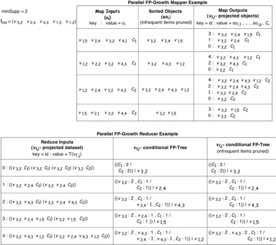
The second MapReduce phase, Parallel FP-Growth, is the core of the CAR Mining process and the relative pseudo-code is reported in Fig. 4. The mapper generates item-projected objects so that reducers can generate con-ditional FP-trees, which are independent of each other during the recursive mining process. Like in the previous phase, each mapper is fed by an HDFS block and the input key-value pair is hkey, value = oii. For each oi, the mapper gets the class label Cli and sorts the feature values according to
the flist. Let soi be the sorted object. Then, for each item soi,p ∈ soi, the mapper outputs the key-value pair hkey = id, value = {soi,1, . . . , soi,p, Cli}i
where id is the index of the item soi,p in the flist and {soi,1, . . . , soi,p, Cli} is
the soi,p-projected object. Since each item is independent of the others, the reducer processes a set of independent projected objects for each single item, which represents the vf,j-projected training set, T(vf,j). The reducer inputs a key-value pair hkey = id, value = T(vf,j)i, builds the local FP-tree and recursively mines the classification association rules as described in [16]. Fi-nally, it returns only the CARs whose support, confidence and χ2 values are greater than the relative thresholds (line 18 in Fig. 4). In particular, reducers output hkey =null, value=CARmi pairs, where CARm is the m-th gener-ated rule. Note that the number of pairshkey, list(values)iprocessed by each reducer is determined by the default partition function hash(key) mod R. Since in Parallel FP-Growth the intermediate key is the specific item index in flist, more or less the same number of pairs hkey, list(values)i, i.e. of conditional FP-Trees, is assigned to each reducer by the partition function. However, such distribution does not necessarily guarantee a perfect load bal-ancing among all the reducers, because the time spent in processing each
specific FP-Tree depends on the number and the length of its paths; more precisely, the relative time complexity is exponential with respect to the longest frequent path in the conditional pattern base [22, 57]. Thus, space and time complexities of each reducer depend on the size and the execution time of all the processed projected training sets, Ored(Sum(|T(vf,j)|)) and Ored(Sum(F P Growth(T(vf,j)))), respectively.
Figure 5 shows a simple example of the Parallel FP-Growth execution, with four objects and minSupp= 2. Mappers sort frequent items according to the flist and create item-projected objects for each item. Reducers build the local conditional FP-Tree for the specific item and recursively mine the candidate rule set. Each node on the FP-Tree represents an item and each path represents an item-projected object. Since different paths share the same prefix, the tree is a compressed view of the vj,i-projected dataset.
The last MapReduce phase, Candidate Rule Filtering, selects only the K most significant non-redundant rules for each class labelCl. A CARm is more significant than another CARs if and only if:
1. conf(CARm)> conf(CARs)
2. conf(CARm) = conf(CARs)AND supp(CARm)> supp(CARs); 3. conf(CARm) = conf(CARs)ANDsupp(CARm) =supp(CARs)AND
RL(CARm)< RL(CARs).
where conf(.), supp(.) and RL(.) are the confidence, the support and the rule length, respectively. A rule CARm :Antm →Clm is more general than
a rule CARs : Ants → Cls, if and only if, Ants ⊆ Antm. A rule CARm is
not inserted into the K most significant non-redundant rules if there exists a rule CARs that is more significant and more general than CARm. This
1: procedure Mapper(key, value =oi) 2: flist ←LoadFrequentItemList();
3: oi[]←Split(oi); .Array of Items
4: Cli ←RemoveLastItem();
5: soi[]←Sort(oi[], flist); .Array of Items Sorted according to flist 6: for p=|soi[]| −1to 0 do
7: id←getIndexFList(soi[p]);
8: Call Output(hkey =id, value={soi[1]. . . soi[p], Cli}i);
9: end for
10: end procedure
11: procedure Reducer(key =id, value=T(vj,i)) 12: F P T ree←newFPTree();
13: for all soi in T(vj,i) do 14: F P T ree←insert(soi);
15: end for
16: CARlist←FPGrowth(F P T ree); 17: for all CARm inCARlist do
18: if isV alid(CARm)then .Check support, confidence and χ2 19: Call Output(hkey =null, value=CARmi);
20: end if
21: end for
22: end procedure
allows us to discard redundant rules and cover a greater number of objects in the training set. Each mapper is fed with the key-value pair in the form of hkey = null, value = CARmi and outputs a pair hkey = Clm, value =
CARmi where Clm is the CARm class label. Each reducer processes all
rules with the same class label, List(CARCl), and selects only the K most
significant non-redundant rules. For each of these K rules the reducer outputs a key-value pairhkey =null, value=CARmi. Fig. 6 shows the pseudo-code of the Candidate Rule Filtering phase. We highlight that, at line 8, if the current ruleCARm can be inserted into the K most significant non-redundant rules, the methodcheckRedundantchecks and removes all rules that become redundant when new CARm is added. Space complexity is O(K) and time complexity isO(M ax(|CARCl|)·log(K)/Q), where Qis the number of CUs.
3.3. Rule Pruning
Rule pruning aims to discard less relevant rules to speed up the classifi-cation process. Pruning has to be applied carefully, avoiding to drop useful knowledge along with discarded rules. Among the approaches proposed for rule pruning it is worth recalling lazy pruning [6], database coverage [3], and pessimistic error estimation [1].
In MRAC three different types of pruning ase used. In the first type, a rule CARm is pruned if its support, confidence and χ2 are not greater than minSupp,minConf andminχ2 thresholds, respectively. This type of pruning
is performed at the end of the Parallel FP-Growth phase, when the rule is mined. Since the support value is stored along the FP-tree, the computation of support, confidence and χ2 can be performed on the fly.
1: procedure Mapper(key, value =CARm) 2: Clm ←getClassLabelRule(CARm);
3: Call Output(hkey =Clm, value=CARmi );
4: end procedure
5: procedure Reducer(key =Cl, value=List(CARCl))
6: HP ←createMaxHeap(K); . K defines the HP size
7: for all CARm inList(CARCl) do
8: if checkRedundant(CARm, HP)then 9: if |HP| < K then
10: HP ←insert(CARm);
11: else
12: if rank(HP[0]) < rank(CARm) then
13: HP ←deleteTopElement(); 14: HP ←insert(CARm); 15: end if 16: end if 17: end if 18: end for
19: for all CARm inHP do
20: Call output(hkey =null, value=CARmi);
21: end for
22: end procedure
candidate rules are sorted according to their ranking position as described in Section 3.2 and only the K most significant non-redundant rules for each class label are selected. Experimentally we found that this second step can reduce significantly the number of CARs in theCARlist, without significantly affecting the classification accuracy. This type of pruning is performed in the reduce phase of the Candidate Rule Filtering job.
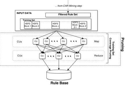
In the third type of pruning, shown in Fig. 7, the training set coverage is exploited: the retained rules are only those that are activated by at least one data object in the training set. Each data object in the training set is associated with a counter initialized to 0. For each object, a scan over the sorted CARlist is performed to find all the rules that match the object. If CARm classifies correctly at least one data object, then CARm is inserted into the rule base. Further, the counters associated with the objects, which activate CARm, are incremented by 1. Whenever the counter of an object becomes larger than thecoverage threshold δ, the data object is removed from the training set and no longer considered for subsequent rules. Since rules are sorted in descending significance, it is very likely that these subsequent rules would have a very limited relevance for the object. The procedure ends when no more objects are in the training set or all the rules have been analyzed.
Fig. 8 shows the MapReduce pseudo-code of the third type of pruning. Each mapper instance loads and ranks into memory the filtered rule set, CARlist, mined in the previous step. Further, since each mapper is fed with an HDFS block, the key-value input pair is hkey = null, value = oii. For each object oi, the mapper sets the counter to 0 and scans the CARlist. If CARm matches oi, then the counter is incremented by 1. Further, if
Figure 7: The Pruning step of the MapReduce Associative Classifier.
CARm also classifies correctly object oi, the mapper outputs to the re-ducer the index indexCARm of CARm in the CARlist and null as,
respec-tively, key and value, that is, hkey = indexCARm, value = nulli. When
the counter overcomes the coverage threshold δ,oi is not processed anymore and the next object is taken into account. The reducer instance retrieves the correct rule from the CARlist and outputs it. The key-value input pair is hkey = indexCARm, value = nulli and the key-value output pair is
hkey = null, value =CARmi. Space complexity is O(N/Q) and time com-plexity in the worst case is O(N· |CARlist|/Q), where|CARlist| ≤L·K and Q is the number of CUs.
3.4. Classification
The pruned set of rules represents the rule base used to classify an un-labeled pattern bx. All rules that match the unlabeled pattern are taken
1: procedure Mapper(key, value =oi)
2: CARlist←loadAndRankFilteredRuleSet(); 3: δ ←loadCoverageThreshold();
4: count←0;
5: for all CARm inCARlist do 6: if CARm matches oi then 7: count←count+ 1;
8: if CARm correctly classifies oi then
9: indexCARm ←getIndex(CARm, CARlist);
10: Call Output(hkey =indexCARm, value=nulli);
11: end if 12: end if 13: if count > δ then 14: break; 15: end if 16: end for 17: end procedure
18: procedure Reducer(key =indexCARm, value=null)
19: CARlist←loadAndRankFilteredRuleSet(); 20: CARm ←getRule(indexCARm, CARlist);
21: Call Output(hkey =null, value=CARmi); 22: end procedure
into account: they can predict either the same class label or different class labels. In the first case, MRAC simply assigns the class label to the unla-beled pattern. In the second case, the algorithm splits the rules into different groups according to the class label and compares the strength strCl of each
group. The strength is computed by adopting the weighted chi-squared [4] as reasoning method: strCl = X CARm∈RB(Cl) χ2 mχ2m maxχ2 m (11)
where RB(Cl) contains all the rules in the rule base with the same class label Cl, which match the unlabeled pattern, and χ2m and maxχ2m are the chi-square and its upper bound for the ruleCARm, respectively. Themaxχ2m for a generic rule CARm :Antm →Clm is calculated as follows:
maxχ2m= (minsupp(Antm, supp(Clm))−
supp(Antm)·supp(Clm)
N )
2·N ·e
(12) wheresupp(Antm) is the support of the antecedent of ruleCARm,supp(Clm)
is the support of the class labelClm,N is the number of objects in the training
set and e is computed as:
e= 1
supp(Antm)·supp(Clm)
+ 1
supp(Antm)·(N −supp(Clm))
+
+ 1
(N −supp(Antm)·supp(Clm)
+ 1
(N−supp(Antm))·(N −supp(Clm))
(13) MRAC assigns the unlabeled pattern to the class label associated with
the top-strength group. In case no rule matches the pattern, the method classifies bxwith the class label with the highest support.
4. Experimental Study
Specific experimental tests have been devised to characterize the behavior of the proposed algorithm, focusing on the following crucial aspects: i) as-sessment of the classification accuracy, ii) horizontal scalability analysis with a typical complete dataset, and iii) study on the ability to efficiently accom-modate an increasing dataset size.
In our tests we made use of 21 classification datasets widely known in the literature, extracted from the UCI repository1, which are characterized
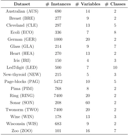
by different numbers of input variables (from 4 to 60) and input/output instances (from 150 to 11000000). Among them, 18 ordinary-sized datasets are reported in Table 1. The last three benchmarks, referring to big data, are shown in Table 2: they are suitable for our proposed algorithm, but not for classical classifiers.
All the experiments have been run using Apache Hadoop 1.0.4 as the reference MapReduce implementation. The chosen testbed corresponds to a typical low-end system suitable for supporting the target classifying service: a small cluster with one master machine and three slave nodes, connected by a Gigabit Ethernet (1 Gbps). All the nodes run Ubuntu 12.04. Regarding the placement of the Hadoop components, the master hosts the NameNode and JobTracker processes, while each slave runs a DataNode and a TaskTracker.
Table 1: Ordinary-sized datasets used in the experiments.
Dataset # Instances # Variables # Classes
Australian (AUS) 690 14 2 Breast (BRE) 277 9 2 Cleveland (CLE) 297 13 5 Ecoli (ECO) 336 7 8 German (GER) 1000 20 2 Glass (GLA) 214 9 7 Heart (HEA) 270 13 2 Iris (IRI) 150 4 3 Led7digit (LED) 500 7 10 New-thyroid (NEW) 215 5 3 Page-blocks (PAG) 5472 10 5 Pima (PIM) 768 8 2 Ring (RING) 7400 20 2 Sonar (SON) 208 60 2 Twonorm (TWO) 7400 20 2 Wine (WIN) 178 13 3 Wisconsin (WIS) 683 9 2 Zoo (ZOO) 101 16 7
Table 2: Large-sized datasets used in big data experiments.
Dataset # Instances # Variables # Classes
HIGGS (HIG) 11000000 28 2 KDDCup DOS vs Normal (KDD) 4856151 41 2
The NameNode is devoted to handling the HDFS, keeping track of its block replicas (64 MB by default), and to coordinating all theDataNode processes as well. The master node has a 4-core CPU (Intel Core i5 CPU 750 x 2.67 GHz), 4 GB of RAM and a 500GB Hard Drive. Each slave node has a 4-core CPU with Hyperthreading (Intel Core i7-2600K CPU x 3.40 GHz), 16GB of RAM and 1 TB Hard Drive.
4.1. Assessing accuracy
To properly assess the accuracy delivered by MRAC, a comparison with other associative classifiers is needed. Thus, MRAC has been compared to the sequential implementation of three different well-known associative classification models, namely CBA [3], CBA2 [58], and CPAR [5].
TheClassification-Based Association (CBA) algorithm mines the rules by using Apriori method; subsequently, it sorts and chooses a set of high precedence rules to cover the entire training dataset. The CBA2 algorithm improves CBA in tuning the minimum support thresholds across different classes [58]. On the contrary, Classification based on predictive association rules (CPAR) generates association rules directly from training data using a greedy algorithm based on the FOIL method [59]. Specifically, multiple literals with similar gains are selected, and multiple rules are accordingly generated at each step. Moreover, it uses only the best D rules to perform the classification task.
In our experiments, we used the implementations of CBA, CBA2 and CPAR available in the KEEL package [60], and the datasets from Table 1 as benchmarks. It is worth mentioning that, to the best of our knowledge, no implementation of ordinary associative classifiers exists that is able to handle
very large amounts of data like those listed in Table 2, which will be used instead for other purposes.
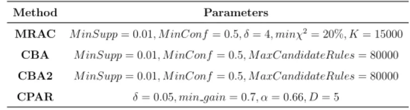
Table 3 summarizes the algorithm parameters used in the experiments: They have been chosen according to the guidelines provided by the authors in the related papers [3, 5, 58]. Further, for each dataset and for each algorithm, we performed a five-fold cross-validation by using the same folds for all the datasets. The discretization of the continuous features has been performed by the entropy-based method proposed by Fayyad and Irani [53] and discussed in Section 3.1.
Table 3: Values of the parameters for each algorithm used in the experiments.
Method Parameters
MRAC M inSupp= 0.01, M inConf= 0.5, δ= 4, minχ2= 20%, K= 15000
CBA M inSupp= 0.01, M inConf= 0.5, M axCandidateRules= 80000 CBA2 M inSupp= 0.01, M inConf= 0.5, M axCandidateRules= 80000
CPAR δ= 0.05, min gain= 0.7, α= 0.66, D= 5
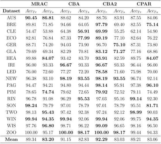
Table 4 shows, for each dataset and for each algorithm, the average values of the accuracy, both on the training (AccT r) and test sets (AccT s) associated with the ACs generated by the four algorithms. The highest accuracy values for each dataset are shown in bold.
By inspecting Table 4 we can see that, in most of the datasets, MRAC is more accurate than the other ACs. Moreover, MRAC achieves the best average accuracy on the test sets. Another significant observation is that both CBA and CBA2 are more prone to overtraining than CPAR and MRAC.
Table 4: Average accuracy achieved by MRAC, CBA, CBA2 and CPAR
MRAC CBA CBA2 CPAR
Dataset AccT r AccT s AccT r AccT s AccT r AccT s AccT r AccT s
AUS 90.45 86.81 88.62 84.20 88.76 83.91 87.55 84.06 BRE 89.81 71.85 94.66 64.05 97.79 69.40 82.55 75.14 CLE 54.47 53.88 64.38 56.91 69.99 55.25 62.14 54.90 ECO 82.81 76.84 87.33 77.99 89.19 77.10 82.64 76.22 GER 88.71 74.20 94.03 73.90 96.70 75.10 87.31 73.80 GLA 79.69 69.34 82.29 70.81 83.12 71.27 77.16 68.86 HEA 89.88 84.07 93.42 83.70 93.91 82.59 89.75 84.07 IRI 96.00 93.33 96.67 93.33 96.67 93.33 96.44 96.00 LED 76.00 72.60 77.27 72.20 78.58 71.60 75.98 70.00 NEW 96.38 93.10 98.19 93.55 98.19 93.55 96.74 92.14 PAG 94.47 94.21 94.80 94.44 98.14 95.91 97.38 96.10 PIM 78.65 74.74 79.62 72.65 79.92 72.52 79.11 74.49 RIN 96.78 91.08 96.29 95.53 97.03 95.16 99.14 92.30 SON 98.24 79.79 97.01 78.79 97.01 78.79 95.51 81.71 TWO 98.13 95.43 97.42 92.38 97.24 92.12 98.99 90.03 WIN 99.94 94.35 99.94 92.06 99.94 92.06 99.75 94.35 WIS 97.76 96.80 98.71 96.22 99.09 96.65 98.16 96.50 ZOO 100.00 95.17 100.00 98.17 100.00 98.17 99.44 94.33 Mean 89.34 83.20 91.15 82.83 92.29 83.03 89.21 83.06
of accuracy on the test set associated with the classifiers generated by the different algorithms, we have performed a statistical analysis. As suggested in [61], we apply non-parametric statistical tests combining all the datasets: for each approach we generate a distribution consisting of the mean values of accuracy calculated on the test set. Then, we apply the Friedman test in order to compute a ranking among the distributions [62], and the Iman and Davenport test [63] to evaluate whether there exist statistically relevant differences among the distributions. If there exists a statistical difference, we apply a post-hoc procedure, namely the Holm test [64]. This test allows detecting effective statistical differences between the control approach, i.e. the one with the lowest Friedman rank, and the remaining approaches.
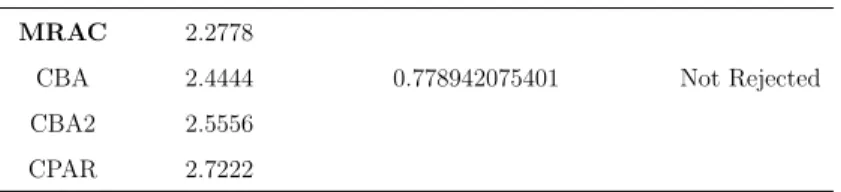
Table 5 shows the results of the non-parametric statistical tests: for each algorithm, we show the Friedman rank and the Iman and Davenportp-value. If the p-value is lower than the level of significance α (in the experiments α = 0.05), we can reject the null hypothesis and affirm that there exist statistical differences between the multiple distributions associated with each approach. Otherwise, no statistical difference exists among the distributions and therefore the associative classifiers are statistically equivalent.
Table 5: Results of the non-parametric statistical tests on the accuracy calculated on the test set
Algorithm Friedman rank Iman and Davenport p-value Hypothesis
MRAC 2.2778
CBA 2.4444 0.778942075401 Not Rejected
CBA2 2.5556
We can observe that no post-hoc procedure has to be applied, because no statistical difference among the four algorithms has been detected. Thus, we can conclude that MRAC achieves accuracies comparable to some classical associative classifiers proposed in the literature.
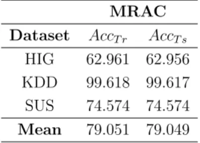
For the sake of completeness, the accuracy achieved by MRAC on the very large datasets in Table 2 has been measured. Also in this case, we performed a five-fold cross-validation for each dataset. Table 6 shows the average accuracy values, both on the training (AccT r) and test sets (AccT s). We do not show the results achieved by CBA, CBA2 and CPAR because the available implementations of these algorithms cannot manage these datasets. We observe that the values obtained on the training and test sets are very similar. This result is a consequence of the size of the dataset and the data distribution. Indeed, since the datasets are very large, the training sets selected in the fold cross-validation result to be a very representative sample of the overall dataset.
Table 6: Average accuracy achieved by MRAC on large datasets.
MRAC
Dataset AccT r AccT s
HIG 62.961 62.956 KDD 99.618 99.617 SUS 74.574 74.574
Mean 79.051 79.049
Summing up, the results obtained by MRAC are statistically equivalent to those achieved by algorithms of the same type, with comparable (or slightly
better) accuracy. On the other hand, its main advantage over the other algorithms is the capability to process huge amounts of data in a reasonable time even on a small-sized cluster of ordinary multicore machines. The next sections are devoted to a precise empirical characterization of this aspect. 4.2. Horizontal scalability analysis
In this section, we investigate on the MRAC behavior in employing addi-tional computing units. To this aim, we measure the values assumed by the speedup σ, taken as the main metrics, commonly used in parallel computing. For the sake of clarity, we report the figures obtained with tests on the Susy dataset; similar results can be recorded with the other datasets.
According to the speedup definition, the efficiency of a program using multiple CUs is calculated comparing the execution time of the parallel im-plementation against the corresponding sequential, “basic” version. In our application setting, because of the large size of the involved datasets, it is not practically sensible to regard the sequential version of the overall algorithm as the basic one (it would take an unreasonable amount of time), so we can refer to a run over Q∗ identical CUs,Q∗ >1. Hence, we adopt the following
slightly different definition for the speedup on n identical CUs: σQ∗(n) =
Q∗·τ(Q∗)
τ(n) (14)
where τ(n) is the program runtime using n CUs, and Q∗ is the number of CUs used to run the reference execution, which lets us estimate a fictitious, ideal single-core runtime as Q∗·τ(Q∗). Of course, σQ∗(n) makes sense only
for n ≥ Q∗. In our case, τ(Q∗) accounts also for the basic overhead due to the Hadoop platform.
For n > Q∗ the speedup is expected to be sub-linear because of the
increasing overhead from the Hadoop procedures, because of the behavior of the algorithm (considering also the granularity of the necessary sequential parts) and, in case of multicore physical nodes, because of contention on resources shared among cores within the same CPU.
In our tests, we assumed Q∗ = 6 to have 2 working cores for each slave available in the cluster and thus accounting in σ6 also for the basic overhead
due to thread interference.
Considering the structure of our algorithm, we set the number of reducers equal to the number of cores and we distribute them uniformly among the slaves.
Horizontal scalability has been studied by varying the number of switched-on cores per node. To avoid unbalanced loads, we recorded the executiswitched-on times experienced with the same number of running cores per node. In practice, we considered 6, 9, and 12 cores distributed on the three slave nodes.
It is worth noticing that the HyperThreading technology was available on our testbed CPUs, which thus might run two distinct processes per core. The performance gain due to HypertThreading highly depends on the target application, and in server benchmarks it reaches 30% [65]. In our case, specific tests showed that HyperThreading yields really limited performance improvements. For this reason we disabled the HyperThreading Technology and used only the available physical CUs in all our experiments.
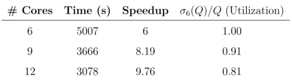
Table 7 and Figure 9 show the speedup according to the whole dataset. With the default Hadoop settings, the number Z of mappers is
auto-Table 7: Speedup for the Susy dataset.
# Cores Time (s) Speedup σ6(Q)/Q (Utilization)
6 5007 6 1.00 9 3666 8.19 0.91 12 3078 9.76 0.81 3000 3500 4000 4500 5000 5500 4 6 8 10 12 14 Runtime (sec) Number of Cores (Q) (a) Runtime 0 2 4 6 8 10 12 14 0 2 4 6 8 10 12 14 Speedup ( σ6 ) Number of Cores (Q) (b) Speedup
matically determined by the HDFS block size. E.g., for the Susy dataset Hadoop instantiates 36 mappers. Furthermore, indicating by Q the number of available cores, ifZ ≤Qthen all the mappers are run simultaneously, and the global runtime practically corresponds to the longest of the mappers’ runtimes. Otherwise (Z > Q), Hadoop starts from executing Q mappers in parallel, queuing the rest (Z −Q). As soon as one of the running mappers completes, Hadoop schedules a new mapper from the queue.
In the ideal case of the same execution time for all the mappers, the map phase for each MapReduce stage would require dZ
Qe iterations. With the Susy dataset, this corresponds to 6, 4 and 3 iterations on 6, 9 and 12 cores, respectively. This observation can be used to get a very rough estimation of the runtime expected with a certain number of cores, once the runtime with another given number of cores has been recorded. Such an estimation cannot be accurate because all the mappers do not have exactly the same execution time (they may even be assigned different input sizes) and because of the influence of the different reducing phases. For instance (see Table 7), we expect that runtime decreases from 5007 seconds with 6 cores to about 5007×4÷6 = 3338 and 5007×3÷6 = 2503 seconds with 9 and 12 cores, respectively. As it can be noticed, such values do not excessively differ from the recorded ones. Of course, the actual runtimes are necessarily higher due to the incurred overheads.
The actual speedup σ6 in our experiments does not excessively diverge
from the ideal value, i.e. the number of CUs2: σ
6(9)/9 = 0.91 andσ6(12)/12 = 2The valueσ
1/Qis the standardutilizationindex; in our case, asσi(n)≤σj(n)∀n≥j, the utilization index σ6/Qmay be slightly greater than standard utilization.
0.81. Within the limitations due to the different experimental settings, this result is in line with [18] where the utilization is 0.768.
A better understanding of the presented overall figures requires a break-down of the contributions from the different parts of the algorithm. To this aim, in Table 8 and Figure 10 we report the speedup σ6 of the most
sig-nificant MapReduce phases: Parallel FP-Growth and Parallel Training Set Coverage Pruning. The contribution of the other two, i.e. Parallel Counting and Candidate Rule Filtering, is negligible (about 2.63% and 1,09% of the overall execution time, respectively).
Table 8: Runtime and speedup of each MRAC phase in the Susy dataset.
Parallel FP-Growth
Training Set Coverage Pruning # Cores Time (s) Speedupσ6 σ6(Q)/Q Time (s) Speedupσ6 σ6(Q)/Q
6 1568 6 1.00 2984 6 1.00
9 1257 7.48 0.83 2059 8.70 0.97
12 1160 8.11 0.67 1614 11.09 0.92
The two charts in Figure 10 clearly show that the two phases behaves differently with respect to scalability.
The speedup ofParallel FP-Growth(Figure 10a) rapidly degrades, mostly because of the computational weight of the reducing activity. In fact, the average runtime of each mapper is quite short (about 40 seconds), and the global execution time is dominated by the mining of CARs from the con-ditional FP-Trees: such an activity is carried out in the reducing phase. With the Hadoop default settings, all the conditional FP-Trees are evenly distributed among the reducers.
0 2 4 6 8 10 12 14 0 2 4 6 8 10 12 14 Speedup ( σ6 ) Number of Cores (Q) (a) Parallel FP-Growth speedup. 0 2 4 6 8 10 12 14 0 2 4 6 8 10 12 14 Speedup ( σ6 ) Number of Cores (Q) (b)
Training Set Coverage Pruning
speedup.
Figure 10: Speedup of the two main MRAC phases
In our tests, Susy has 146 frequent items, thus each reducer processes 24, 16 and 12 FP-Trees in the 6, 9 and 12 cores cases, respectively. InParallel FP-Growth, adding more cores helps us improve the FP-Growth parallelization, decreasing the number of conditional FP-Trees processed by each reducer.
Conversely, the Training Set Coverage Pruning is driven by the map phase, with very satisfactory utilization values. In this case, the average runtime of each mapper is around 7 minutes. The global execution time can be shrunk by reducing the number of iterations, i.e. by exploiting additional CUs, as witnessed by the results in Table 8.
4.3. Tackling the dataset size
From a practical point of view, it is crucial to understand how the pro-posed algorithm behaves as the input dataset size grows up. To test this aspect, we extracted differently sized datasets out of Susy. For each given size, three different experiments have been executed on three distinct subsets of Susy, with records randomly sampled out of the complete dataset. We
in-dicate a subset with x% of the records in Susy by the notation Susyx; thus, the complete dataset is Susy100.
Table 9 and Figure 11 show the average runtime for building the rule base, according to different problem sizes and number of cores.
Table 9: Average runtime of MRAC on Susy dataset, varying dataset size and number of available cores.
Dataset Number of Cores
Size (%) Objects Mappers 6 9 12
10 (Susy10) 500,000 4 751 733 745
25 (Susy25) 1,250,000 9 1309 862 855
50 (Susy50) 2,500,000 18 2239 1677 1513
75 (Susy75) 3,750,000 27 3481 2591 2404
100 (Susy100) 5,000,000 36 5007 3666 3078
As shown forSusy10and Susy25, whenever the number of available cores
Q is sufficient to run all the mappers in parallel, adding more cores does not trivially yield any benefit. When the number of mappers exceeds the number of cores, Hadoop queues up the extra mappers to be subsequently scheduled when cores become available again. Thus, as long as the number of mappers’ iterations is the same, no significant gain is expected by adding new cores. For instance, for Susy50 passing from 9 to 12 cores is of little practical use,
since the number of parallel mapper iterations (namely, two) does not change. In this case, runtime improves only of 150 seconds. On the other hand, the runtime difference passing from 6 to 9 cores is more significant (about 600
1000 2000 3000 4000 5000 0*100 1*106 2*106 3*106 4*106 5*106 Runtime (sec)
Dataset Size (Number of objects)
6 cores 9 cores 12 cores
seconds), because a reduction of the number of parallel mapper iterations occurs (from 3 to 2). Similar considerations can be made for Susy75 and
Susy100. Note that in the last case, passing from 6 to 9 cores determines a
reduction of iterations from 6 to 4, while adding yet other three cores the iterations just go down to 3, i.e. yielding half the previous gain.
Experiments show that as the dataset size grows up, the execution time can be effectively reduced by adding a proper number of additional cores, at least whenever dealing with sizes typical of current big data benchmarks. In particular, performance improvements are mainly related to the reduction in the number of parallel mapper iterations spent by the algorithm to scan the overall dataset.
5. Conclusions
In this paper we have presented MRAC, a MapReduce associative clas-sifier based on frequent pattern mining. MRAC first extracts the frequent items. Then, it generates the top-K significant classification association rules from them by exploiting a parallel version of the well-known FP-Growth al-gorithm. Finally, it prunes noisy and redundant rules by applying a parallel dataset coverage technique. We have shown that MRAC achieves accura-cies comparable with the ones obtained by other associative classifiers on some datasets commonly used as benchmark. Furthermore, MRAC is able to process millions of data for learning the classification association rules. On the other hand, the MapReduce framework provides a robust and trans-parent environment to parallelize the computation flow across large-scale clusters of machines, taking care of communications between them and
pos-sible failures. Experimental results performed on three big datasets show that MRAC achieves speedup and scalability close to the ideal achievable targets. We would like to highlight that these results are obtained by us-ing personal computers connected by a Gigabit Ethernet and not specific dedicated hardware.
As future work, we aim to experiment MRAC on a larger number of big datasets, investigating scalability, speedup and load balance on each MapRe-duce stage by employing a larger cluster of machines.
References
[1] I. H. Witten, E. Frank, Data Mining: Practical Machine Learning Tools and Techniques, 3rd Edition, Morgan Kaufmann Series in Data Man-agement Sys, Morgan Kaufmann, 2011.
[2] R. Agrawal, T. Imieli´nski, A. Swami, Mining association rules between sets of items in large databases, SIGMOD Record 22 (2) (1993) 207–216. doi:10.1145/170036.170072.
[3] B. Liu, W. Hsu, Y. Ma, Integrating classification and association rule mining, in: Proceedings of the Fourth International Conference on Knowledge Discovery and Data Mining, 1998, pp. 80–86.
[4] W. Li, J. Han, J. Pei, CMAR: accurate and efficient classification based on multiple class-association rules, in: Proceedings of IEEE International Conference on Data Mining 2001, 2001, pp. 369–376. doi:10.1109/ICDM.2001.989541.
[5] X. Yin, J. Han, CPAR: Classification based on predictive association rules, in: Proceedings of the third SIAM international conference on data mining, 2003, pp. 331–335. doi:10.1137/1.9781611972733.40. [6] E. Baralis, P. Garza, A lazy approach to pruning classification rules, in:
Proceedings of 2002 IEEE International Conference on Data Mining, 2002, pp. 35–42. doi:10.1109/ICDM.2002.1183883.
[7] N. Abdelhamid, A. Ayesh, F. Thabtah, S. Ahmadi, W. Hadi, MAC: A multiclass associative classification algorithm, Journal of Information & Knowledge Management 11 (02). doi:10.1142/S0219649212500116. [8] A. Veloso, W. Meira Jr., M. J. Zaki, Lazy associative classification,
in: Proceedings of the Sixth International Conference on Data Mining, ICDM ’06, IEEE Computer Society, Washington, DC, USA, 2006, pp. 645–654. doi:10.1109/ICDM.2006.96.
[9] J. R. Quinlan, C4.5: Programs for Machine Learning, Morgan Kauf-mann Publishers Inc., San Francisco, CA, USA, 1993.
[10] Y. Sun, Y. Wang, A. K. Wong, Boosting an associative classifier, Knowl-edge and Data Engineering, IEEE Transactions on 18 (7) (2006) 988– 992. doi:10.1109/TKDE.2006.105.
[11] L. T. Nguyen, B. Vo, T.-P. Hong, H. C. Thanh, CAR-miner: An effi-cient algorithm for mining class-association rules, Expert Systems with Applications 40 (6) (2013) 2305–2311. doi:10.1016/j.eswa.2012.10.035. [12] M. I. A. Ajlouni, W. Hadi, J. Alwedyan, Detecting phishing websites
using associative classification, European Journal of Business and Man-agement 5 (15) (2013) 36–40.
[13] G. Costa, R. Ortale, E. Ritacco, X-Class: Associative classification of XML documents by structure, ACM Transactions on Information Sys-tems 31 (1) (2013) 3:1–3:40. doi:10.1145/2414782.2414785.
[14] Y. Yoon, G. G. Lee, Two scalable algorithms for associative text classifi-cation, Information Processing and Management 49 (2) (2013) 484–496. doi:10.1016/j.ipm.2012.09.003.
[15] S. Dua, H. Singh, H. Thompson, Associative classification of mammo-grams using weighted rules, Expert Systems with Applications 36 (5) (2009) 9250–9259. doi:10.1016/j.eswa.2008.12.050.
[16] J. Han, J. Pei, Y. Yin, R. Mao, Mining frequent patterns without can-didate generation: A frequent-pattern tree approach, Data Min. Knowl. Discov. 8 (1) (2004) 53–87. doi:10.1023/B:DAMI.0000005258.31418.83. [17] J. P. J. Han, M. Kamber, Data Mining: Concepts and Techniques, 3rd
Edition, Data Management Systems, Morgan Kaufmann, 2012.
[18] H. Li, Y. Wang, D. Zhang, M. Zhang, E. Y. Chang, PFP: Parallel FP-Growth for query recommendation, in: Proceedings of the 2008 ACM Conference on Recommender Systems, RecSys ’08, ACM, New York, NY, USA, 2008, pp. 107–114. doi:10.1145/1454008.1454027.
[19] W. Fan, A. Bifet, Mining big data: Current status, and fore-cast to the future, SIGKDD Explor. Newsl. 14 (2) (2013) 1–5. doi:10.1145/2481244.2481246.
[20] L. Liu, E. Li, Y. Zhang, Z. Tang, Optimization of frequent itemset min-ing on multiple-core processor, in: Proceedmin-ings of the 33rd International Conference on Very Large Data Bases, VLDB ’07, VLDB Endowment, 2007, pp. 1275–1285.
[21] O. Zaiane, M. El-Hajj, P. Lu, Fast parallel association rule mining without candidacy generation, in: Data Mining, 2001. ICDM 2001, Proceedings IEEE International Conference on, 2001, pp. 665–668. doi:10.1109/ICDM.2001.989600.
[22] I. Pramudiono, M. Kitsuregawa, Parallel FP-Growth on PC cluster, in: Advances in Knowledge Discovery and Data Mining, Vol. 2637 of Lecture Notes in Computer Science, Springer Berlin Heidelberg, 2003, pp. 467– 473. doi:10.1007/3-540-36175-8 47.
[23] G. Buehrer, S. Parthasarathy, S. Tatikonda, T. Kurc, J. Saltz, Toward terabyte pattern mining: An architecture-conscious solution, in: Pro-ceedings of the 12th ACM SIGPLAN Symposium on Principles and Practice of Parallel Programming, PPoPP ’07, ACM, New York, NY, USA, 2007, pp. 2–12. doi:10.1145/1229428.1229432.
[24] S. O. M. Snir, MPI-The Complete Reference: The MPI Core, MIT Press, 1998.
[25] J. Dean, S. Ghemawat, MapReduce: Simplified data process-ing on large clusters, Commun. ACM 51 (1) (2008) 107–113. doi:10.1145/1327452.1327492.
[27] J. Dean, S. Ghemawat, MapReduce: A flexible data processing tool, Commun. ACM 53 (1) (2010) 72–77. doi:10.1145/1629175.1629198. [28] W. Zhao, H. Ma, Q. He, Parallel K-Means clustering based on
MapRe-duce, in: Cloud Computing, Vol. 5931 of Lecture Notes in Computer Science, Springer Berlin Heidelberg, 2009, pp. 674–679. doi:10.1007/978-3-642-10665-1 71.
[29] N. K. Alham, M. Li, Y. Liu, S. Hammoud, A MapReduce-based dis-tributed SVM algorithm for automatic image annotation, Computers & Mathematics with Applications 62 (7) (2011) 2801–2811, comput-ers & Mathematics in Natural Computation and Knowledge Discovery. doi:10.1016/j.camwa.2011.07.046.
[30] G. Caruana, M. Li, M. Qi, A MapReduce based parallel SVM for large scale spam filtering, in: Fuzzy Systems and Knowledge Discov-ery (FSKD), 2011 Eighth International Conference on, Vol. 4, 2011, pp. 2659–2662. doi:10.1109/FSKD.2011.6020074.
[31] Q. He, C. Du, Q. Wang, F. Zhuang, Z. Shi, A parallel incremental extreme SVM classifier, Neurocomputing 74 (16) (2011) 2532–2540, ad-vances in Extreme Learning Machine: Theory and Applications Biologi-cal Inspired Systems. Computational and Ambient Intelligence Selected papers of the 10th International Work-Conference on Artificial Neural Networks (IWANN2009). doi:10.1016/j.neucom.2010.11.036.
[32] C. Zhang, F. Li, J. Jestes, Efficient parallel kNN joins for large data in MapReduce, in: Proceedings of the 15th International Conference
on Extending Database Technology, EDBT ’12, ACM, New York, NY, USA, 2012, pp. 38–49. doi:10.1145/2247596.2247602.
[33] L. Li, M. Zhang, The strategy of mining association rule based on cloud computing, in: Business Computing and Global Informatiza-tion (BCGIN), 2011 InternaInformatiza-tional Conference on, 2011, pp. 475–478. doi:10.1109/BCGIn.2011.125.
[34] M.-Y. Lin, P.-Y. Lee, S.-C. Hsueh, Apriori-based frequent itemset min-ing algorithms on MapReduce, in: Proceedmin-ings of the 6th International Conference on Ubiquitous Information Management and Communica-tion, ICUIMC ’12, ACM, New York, NY, USA, 2012, pp. 76:1–76:8. doi:10.1145/2184751.2184842.
[35] I. Palit, C. K. Reddy, Scalable and parallel boosting with MapReduce, Knowledge and Data Engineering, IEEE Transactions on 24 (10) (2012) 1904–1916. doi:10.1109/TKDE.2011.208.
[36] C.-T. Chu, S. K. Kim, Y.-A. Lin, Y. Yu, G. R. Bradski, A. Y. Ng, K. Olukotun, Map-Reduce for machine learning on multicore, in: B. Sch¨olkopf, J. C. Platt, T. Hoffmanan (Eds.), Advances in Neural Information Processing Systems 19, Proceedings of the Twentieth An-nual Conference on Neural Information Processing Systems Vancouver, British Columbia, Canada, December 4-7, 2006, MIT Press, 2006, pp. 281–288.
[38] L. Neumeyer, B. Robbins, A. Nair, A. Kesari, S4: Dis-tributed stream computing platform, in: Data Mining Workshops (ICDMW), 2010 IEEE International Conference on, 2010, pp. 170–177. doi:10.1109/ICDMW.2010.172.
[39] Apache storm, https://storm.apache.org (Accessed: December 2014). [40] S. Melnik, A. Gubarev, J. J. Long, G. Romer, S. Shivakumar, M. Tolton,
T. Vassilakis, Dremel: Interactive analysis of web-scale datasets, Proc. VLDB Endow. 3 (1-2) (2010) 330–339. doi:10.14778/1920841.1920886. [41] Apache drill, http://drill.apache.org (Accessed: December 2014). [42] T. White, Hadoop: The Definitive Guide, 3rd Edition, O’Reilly Media,
Inc, 2012.
[43] Apache pig, http://pig.apache.org (Accessed: December 2014). [44] Apache hive, https://hive.apache.org (Accessed: December 2014). [45] Apache hbase, http://hbase.apache.org (Accessed: December 2014). [46] Apache zookeeper, http://zookeeper.apache.org (Accessed: December
2014).
[47] Apache mahout, http://mahout.apache.org (Accessed: December 2014). [48] T. D. Sean Owen, Robin Anil, E. Friedman, Mahout in Action, Manning
Publications Co., 2011.
[49] A. Bifet, G. Holmes, R. Kirkby, B. Pfahringer, MOA: Massive online analysis, J. Mach. Learn. Res. 11 (2010) 1601–1604.
[50] Vowpal wabbit, http://hunch.net/ vw/ (Accessed: December 2014). [51] U. Kang, D. Chau, C. Faloutsos, Pegasus: Mining billion-scale
graphs in the cloud, in: Acoustics, Speech and Signal Processing (ICASSP), 2012 IEEE International Conference on, 2012, pp. 5341– 5344. doi:10.1109/ICASSP.2012.6289127.
[52] Y. Low, J. Gonzalez, A. Kyrola, D. Bickson, C. Guestrin, J. M. Heller-stein, GraphLab: A new framework for parallel machine learning, CoRR abs/1006.4990.
[53] U. M. Fayyad, K. B. Irani, Multi-interval discretization of continuous-valued attributes for classification learning, in: Proceedings of IJCAI, 1993, pp. 1022–1029.
[54] E. J. Clarke, B. A. Barton, Entropy and MDL discretization of con-tinuous variables for bayesian belief networks, International Journal of Intelligent Systems 15 (1) (2000) 61–92.
[55] J. Dougherty, R. Kohavi, M. Sahami, Supervised and unsupervised dis-cretization of continuous features, in: Proceedings of the Twelfth In-ternational Conference on Machine Learning, Morgan Kaufmann, 1995, pp. 194–202.
[56] S. Kotsiantis, D. Kanellopoulos, Discretization techniques: A recent survey, GESTS International Transactions on Computer Science and Engineering 32 (1) (2006) 47–58.
[57] L. Zhou, Z. Zhong, J. Chang, J. Li, J. Huang, S. Feng, Balanced parallel FP-Growth with MapReduce, in: Proc. of 2010 IEEE Youth Conference
on Information Computing and Telecommunications (YC-ICT), 2010, pp. 243–246. doi:10.1109/YCICT.2010.5713090.
[58] B. Liu, Y. Ma, C.-K. Wong, Classification using association rules: Weak-nesses and enhancements, in: R. Grossman, C. Kamath, P. Kegelmeyer, V. Kumar, R. Namburu (Eds.), Data Mining for Scientific and Engi-neering Applications, Vol. 2 of Massive Computing, Springer US, 2001, pp. 591–605. doi:10.1007/978-1-4615-1733-7 30.
[59] J. R. Quinlan, R. M. Cameron-jones, Foil: A midterm report, in: In Proceedings of the European Conference on Machine Learning, Springer-Verlag, 1993, pp. 3–20.
[60] J. Alcal´a-Fdez, L. S´anchez, S. Garc´ıa, M. Jesus, S. Ventura, J. Garrell, J. Otero, C. Romero, J. Bacardit, V. Rivas, J. Fern´andez, F. Herrera, KEEL: a software tool to assess evolutionary algorithms for data mining problems, Soft Computing 13 (3) (2009) 307–318. doi:10.1007/s00500-008-0323-y.
[61] J. Derrac, S. Garc´ıa, D. Molina, F. Herrera, A practical tutorial on the use of nonparametric statistical tests as a methodology for comparing evolutionary and swarm intelligence algorithms, Swarm and Evolution-ary Computation 1 (1) (2011) 3–18. doi:10.1016/j.swevo.2011.02.002. [62] M. Friedman, The use of ranks to avoid the assumption of normality
implicit in the analysis of variance, Journal of the American Statistical Association 32 (200) (1937) 675–701.
[63] R. L. Iman, J. M. Davenport, Approximations of the critical region of the fbietkan statistic, Communications in Statistics - Theory and Methods 9 (6) (1980) 571–595. doi:10.1080/03610928008827904.
[64] S. Holm, A simple sequentially rejective multiple test procedure, Scan-dinavian Journal of Statistics 6 (2) (1979) 65–70.
[65] D. T. Marr, F. Binns, D. L. Hill, G. Hinton, D. A. Koufaty, A. J. Miller, M. Upton, Hyper-Threading technology architecture and microarchitec-ture, Intel Technology Journal 6 (1) (2002) 4–15.