Publications
1-29-2019
Two-Stage Bagging Pruning for Reducing the Ensemble Size and
Two-Stage Bagging Pruning for Reducing the Ensemble Size and
Improving the Classification Performance
Improving the Classification Performance
Hua Zhang
Zhejiang Gongshang University, [email protected]
Yujie Song
Zhejiang Gongshang University
Bo Jiang
Zhejiang Gongshang University
Bi Chen
Zhejiang Gongshang University
Guogen Shan
University of Nevada, Las Vegas, [email protected]
Follow this and additional works at: https://digitalscholarship.unlv.edu/env_occ_health_fac_articles Part of the Data Storage Systems Commons, and the Environmental Public Health Commons
Repository Citation
Repository Citation
Zhang, H., Song, Y., Jiang, B., Chen, B., Shan, G. (2019). Two-Stage Bagging Pruning for Reducing the Ensemble Size and Improving the Classification Performance. Mathematical Problems in Engineering, 2019 1-17. Hindawi Publishing Corporation.
http://dx.doi.org/10.1155/2019/8906034
This Article is protected by copyright and/or related rights. It has been brought to you by Digital Scholarship@UNLV with permission from the rights-holder(s). You are free to use this Article in any way that is permitted by the copyright and related rights legislation that applies to your use. For other uses you need to obtain permission from the rights-holder(s) directly, unless additional rights are indicated by a Creative Commons license in the record and/ or on the work itself.
This Article has been accepted for inclusion in Environmental & Occupational Health Faculty Publications by an authorized administrator of Digital Scholarship@UNLV. For more information, please contact
Research Article
Two-Stage Bagging Pruning for Reducing the Ensemble Size and
Improving the Classification Performance
Hua Zhang
,
1Yujie Song,
1Bo Jiang
,
1Bi Chen,
1and Guogen Shan
21School of Computer and Information Engineering, Zhejiang Gongshang University, Hangzhou, Zhejiang 310018, China 2School of Community Health Sciences, University of Nevada Las Vegas, Las Vegas, NV 89154, USA
Correspondence should be addressed to Hua Zhang; [email protected]
Received 10 July 2018; Accepted 27 December 2018; Published 29 January 2019
Academic Editor: Akhil Garg
Copyright © 2019 Hua Zhang et al. This is an open access article distributed under the Creative Commons Attribution License, which permits unrestricted use, distribution, and reproduction in any medium, provided the original work is properly cited. Ensemble methods, such as the traditional bagging algorithm, can usually improve the performance of a single classifier. However, they usually require large storage space as well as relatively time-consuming predictions. Many approaches were developed to reduce the ensemble size and improve the classification performance by pruning the traditional bagging algorithms. In this article, we proposed a two-stage strategy to prune the traditional bagging algorithm by combining two simple approaches: accuracy-based pruning (AP) and distance-based pruning (DP). These two methods, as well as their two combinations, “AP+DP” and “DP+AP” as the two-stage pruning strategy, were all examined. Comparing with the single pruning methods, we found that the two-stage pruning methods can furthermore reduce the ensemble size and improve the classification. “AP+DP” method generally performs better than the “DP+AP” method when using four base classifiers: decision tree, Gaussian naive Bayes, K-nearest neighbor, and logistic regression. Moreover, as compared to the traditional bagging, the two-stage method “AP+DP” improved the classification accuracy by 0.88%, 4.06%, 1.26%, and 0.96%, respectively, averaged over 28 datasets under the four base classifiers. It was also observed that “AP+DP” outperformed other three existing algorithms Brag, Nice, and TB assessed on 8 common datasets. In summary, the proposed two-stage pruning methods are simple and promising approaches, which can both reduce the ensemble size and improve the classification accuracy.
1. Introduction
Aiming at improving the predictive performance, ensemble methods with bagging [1] and boosting [2, 3] as represen-tatives are in general constructed with a linear combination of a set of fitting models, instead of a single fit of a base classifier or learner [4, 5]. It is well known that an ensemble is usually much more accurate than a single (weaker) learner [1, 6, 7]. Numerous fitting models are generated to reduce the classification error as small as possible with a large ensemble size [8]. As a result, this potentially requires large space for storing the ensemble models, which are often relatively often time-consuming for practical application [9]. On the other hand, these drawbacks can be resolved by removing a part of base classifiers (learners or models) from the original ensemble without loss of predictive performance, which is called ensemble pruning [9–13]. An obvious benefit of ensemble pruning is to fit a relatively small-scale ensemble,
which can not only reduce the storage space and improve the computational efficiency, but also increase the generalization of the pruned ensemble when compared with the original one [5].
The traditional bagging algorithm (also known as boot-strap aggregating) [1], as representatively the simplest ensem-ble method, is composed of two key ingredients, bootstrap and aggregation. Specifically, a number of data subsets for training base learners are independently generated from the original training dataset using the bootstrap sampling [14] with replacement. Then, the bagging algorithm aggregates the outputs of all base learners using voting strategy for classification tasks [5]. Although different sampling strategies have been proposed, for instance, neighborhood sampling in bagging [15], they always lead to large space requirement for storing the base learners and time-consuming computational cost for predictions. In the past decade, therefore, several studies have drawn attention to the bagging pruning for
Volume 2019, Article ID 8906034, 17 pages https://doi.org/10.1155/2019/8906034
reducing the ensemble size as well as retaining or improving the classification performance [16]. For example, Hothorn and Lausen (2003) [17] proposed a double-bagging method to deal with the problems of variable and model selection bias. This approach combined linear discriminant analysis and classification trees to generate ensemble machines. Further-more, Zhang et al. (2009) [10] extended their work by using boosting to prune the double-bagging ensembles. Zhang and Ishikawa (2007) [18] used a hybrid real-coded genetic algorithm to prune the bagging ensemble. Hern´andez-Lobato et al. (2011) adopted either semidefinite programming or ordered aggregation strategies to identify an optimal subset of regressors in a regression bagging ensemble. Xie et al. (2012) [8] introduced an ensemble pruning method, called MAD-Bagging. It utilized the margin distribution based classifi-cation loss as the optimization objective. Chung and Kim (2015) [19] suggested a PL-bagging method that employed positive Lasso to assign weights to base learners in the combination step. Over recent years, Galar et al. (2016) [20] designed an ordering-based ensemble pruning for imbal-anced datasets. Zhang et al. (2017) [21] introduced a novel ensemble pruning techniques called PST2E to obtain smaller but stronger variable selection ensembles. Jiang et al. (2017) [22] proposed a novel strategy of pruning forest to enhance ensemble generalization ability and reduce ensemble size. Onan et al. (2017) [23] proposed a hybrid ensemble pruning approach based on consensus clustering and multiobjective evolutionary algorithm. Guo et al. (2018) [24] presented a margin and diversity based ordering ensemble pruning. Although these pruning methods for bagging can improve the performance of the traditional bagging, the majority of them are relatively complicated and not intuitive for practical use. Furthermore, there are even no suitable model (learner) selections for unknown samples with specificity.
In this work, we proposed a two-stage bagging pruning approach, which is actually composed of two independent methods: accuracy-based pruning (AP) and distance-based pruning (DP). These two methods can be performed by a combination way in any order that finally comprised the two-stage strategy. The former, i.e., the AP procedure, used similar rule as the nice bagging [25] and the trimmed bagging [26] by excluding the worst classifiers and aggregated the rest. Specially, for all models established in the traditional bagging, those base models that had the highest prediction performance measured using accuracy (or the lowest error rates) validated on their out-of-bag samples were selected and retained. For the latter, i.e., the DP procedure, we utilized the specificity of a test sample to select a part of fitting models in the ensemble. This kind of specificity is simply measured as the Euclidean distance between the test sample and the center of the out-of-bag samples corresponding to each model in the traditional bagging. The models closer to the test sample (with smaller distance values) were col-lected to establish the final ensemble for label prediction. Unlike other existing pruning methods, we adopted these two simple and intuitive rules to implement the two-stage bagging pruning strategy aiming at building a novel ensemble method with reduced ensemble size and higher prediction performance.
The remainder of this paper is organized as follows: Section 2 briefly introduced traditional bagging algorithms and measures to evaluate the classification performance. Section 3 described our proposed algorithms for the bagging pruning methods. In Section 4, experimental results and analysis were reported on twenty-eight real datasets. The conclusion was drawn in Section 5.
2. Preliminaries
In this section, we first introduce the traditional bagging algorithm as well as some basic concepts including accuracy, relative improvement, and cross validation for classification task.
2.1. Traditional Bagging Algorithm. Ensemble learning refers to a combination of several relatively weak classifiers to produce a stronger classifier, which can ensure the diversity of weak classifiers and improve the generalization ability. Bagging is one of the basic algorithms for ensemble learning [27], which usually can effectively realize the advantage of an ensemble model [28, 29].
The traditional bagging algorithm is composed of two key ingredients, i.e., bootstrap and aggregation. Firstly, a number of subsets are randomly and independently sampled from the original training set using bootstrap sampling strategy [14] with replacement. Secondly, the bagging algorithm aggre-gates the outputs of all base models using a voting strategy for classification task [5]. The algorithm for the traditional bagging is briefly described as Algorithm 1. Suppose that the training set for a C-class classification problem is given as𝐷 = {(𝑥𝑖, 𝑦𝑖) | 𝑥𝑖 ∈ 𝑅𝑑, 𝑦
𝑖∈ {1, 2, . . . , 𝐶}, 𝑖 = 1, 2, . . . , 𝑁}, where (𝑥𝑖,𝑦𝑖) represents a sample encoded by the 𝑑-dimensional feature vector𝑥𝑖with class label𝑦𝑖, and𝑁is the number of samples in the training set. In addition, assume that 𝐸𝑆 is the original ensemble size which equals to the number of the sampled subsets as well as the number of base classifiers,𝐿 is the base classifier,𝐵represents the ensemble model built with the bagging algorithm, and 𝐵𝑜𝑜𝑡𝑠𝑡𝑟𝑎𝑝 (𝐷) returns a bootstrapped subset generated from the original training set 𝐷.
2.2. Performance Evaluation. To evaluate the prediction per-formance of the proposed pruning methods, we adopted two measures accuracy and relative improvement to assess the classification results.
2.2.1. Accuracy. When a model trained based on a training set is applied to predict a test set, the following measure, called accuracy defined as follows, is used to assess the total classification performance on the test set:
𝐴𝑐𝑐 =𝐶𝑜𝑟𝑟𝑒𝑐𝑡𝑙𝑦 𝑝𝑟𝑒𝑑𝑖𝑐𝑡𝑒𝑑 𝑛𝑢𝑚𝑏𝑒𝑟 𝑜𝑓 𝑠𝑎𝑚𝑝𝑙𝑒𝑠𝑡𝑜𝑎𝑙 𝑛𝑢𝑚𝑏𝑒𝑟 𝑜𝑓 𝑠𝑎𝑚𝑝𝑙𝑒𝑠 × 100%
Input:𝐷-training set,𝐸𝑆- number of the sampled subsets or base models,𝐿- base learner
Output:𝑀-a set of base models,𝐵- bagging ensemble
1 Initialize𝑀 = 0.
2 for𝑖 ∈ {1, 2, . . . , 𝐸𝑆}do:
3 Randomly generate a subset𝐷𝑖=𝐵𝑜𝑜𝑡𝑠𝑡𝑟𝑎𝑝(𝐷)
4 Base model𝑚𝑖= 𝐿(𝐷𝑖)is established using base classifier𝐿trained on the subset𝐷𝑖
5 𝑀 = 𝑀 ∪ {𝑚𝑖}
6 The outcome𝐵(𝑥)of a test sample𝑥predicted by the ensemble model𝐵is given as follows:
𝐵(𝑥) =majority class in{𝑚𝑖(𝑥)}𝑖=1,2,...,𝐸𝑆
Algorithm 1: Traditional bagging algorithm.
2.2.2. Relative Improvement. In this work, we proposed four types of pruning algorithms to reduce the ensemble size and improve the classification performance of the original bagging. We also compared our methods with other three variations of bagging algorithms in Section 4.4. To gain a consistent comparison among these variations or pruned bagging methods, we utilized the same measure as in Croux et al. (2007) [26], called relative improvement. It was defined in terms of the error rate (ER) as follows:
𝑅𝑒𝑙𝑎𝑡𝑖V𝑒 𝑖𝑚𝑝𝑟𝑜V𝑒𝑚𝑒𝑛𝑡
= 𝐸𝑅𝑡𝑟𝑎𝑑𝑖𝑡𝑖𝑜𝑛𝑎𝑙 𝑏𝑎𝑔𝑔𝑖𝑛𝑔− 𝐸𝑅𝑝𝑟𝑢𝑛𝑒𝑑 𝑏𝑎𝑔𝑔𝑖𝑛𝑔 𝐸𝑅𝑡𝑟𝑎𝑑𝑖𝑡𝑖𝑜𝑛𝑎𝑙 𝑏𝑎𝑔𝑔𝑖𝑛𝑔 × 100%
(2)
where 𝐸𝑅𝑡𝑟𝑎𝑑𝑖𝑡𝑖𝑜𝑛𝑎𝑙 𝑏𝑎𝑔𝑔𝑖𝑛𝑔means the error rate of the tradi-tional bagging, which is actually equal to 1- Acc. Sometimes, the performance improvement can also be computed as the relatively accuracy improvement of the pruned bagging with respect to the traditional bagging for comparison and evaluation: 𝐴𝑐𝑐𝑢𝑟𝑎𝑐𝑦 𝑖𝑚𝑝𝑟𝑜V𝑒𝑚𝑒𝑛𝑡 =𝐴𝑐𝑐𝑝𝑟𝑢𝑛𝑒𝑑 𝑏𝑎𝑔𝑔𝑖𝑛𝑔𝐴𝑐𝑐 − 𝐴𝑐𝑐𝑡𝑟𝑎𝑑𝑖𝑡𝑖𝑜𝑛𝑎𝑙 𝑏𝑎𝑔𝑔𝑖𝑛𝑔 𝑡𝑟𝑎𝑑𝑖𝑡𝑖𝑜𝑛𝑎𝑙 𝑏𝑎𝑔𝑔𝑖𝑛𝑔 × 100 % (3)
Consequently, in this work, relative improvement is referred to the definition in terms of error rate and accuracy improvement means the relative increase on accuracy. 2.2.3. Cross Validation. To avoid the overfitting problem in the computational simulations, we used cross validation method to verify the performance of the classifiers or the proposed pruning algorithms. Cross validation [30, 31] is a procedure that divides the training dataset into several subsets and that has three categories [32]: hold-out, K-fold cross validation, and leave-one-out cross validation. How-ever, the way using hold-out is not entirely convincing [33, 34] and the procedure using leave-one-out cross validation is time-consuming for large-scale datasets [33]. Thus, in this work, we adopted K-fold cross validation to evaluate the classification performance of the proposed bagging pruning methods. The K-fold cross validation divides the original dataset into K subsets with even number of samples. Then
one subset is used for test and all the remaining subsets are combined as a training dataset. Repeat such procedure for each subset and calculate the classification performance in each fold. The average accuracy over K folds is finally computed as the classification performance of the proposed method. In this work, fivefold cross validation was applied to all computational experiments.
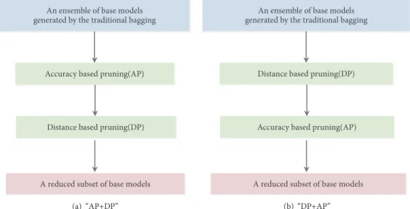
3. Two-Stage Pruning Algorithms for Bagging
We presented two-stage pruning methods according to cer-tain rules to reduce the ensemble size of the traditional bagging algorithm. The proposed two-stage pruning methods are composed of two individual pruning procedures with different rules. The first one is accuracy based, denoted by AP stage, and the second is distance based, named as DP stage. The combinations of these two pruning approaches, called two-stage pruning methods, can be in two forms, i.e., “AP+DP” and “DP+AP”. The form “AP+DP” means that the traditional bagging is firstly pruned using the (accuracy-based) AP pruning method and then DP pruning (distance based) is furthermore performed to reduce the subset of base models derived by AP pruning stage, vice versa for “DP+AP”. The flow diagrams of the two-stage pruning methods “AP+DP” and “DP+AP” were depicted in Figures 1(a) and 1(b), respectively. In this section, we described the algorithms for all of these pruning methods, including AP, DP, “AP+DP”, and “DP+AP”.3.1. Accuracy-Based Pruning Method (AP). The AP procedure adopted similar reduction rule as nice bagging (Nice) [25] and trimmed bagging (TB) [26] in which only good or “nice” bootstrap versions of the base models validated on out-of-bag samples were aggregated. Specially, those base models generated in the traditional bagging, which performed better than the rest ones according to certain decile value𝑡𝑎, were retained to comprise the final reduced set of base models. The main difference among AP, Nice and TB is that different threshold strategy is used to aggregate the “nice” base models. The AP procedure in detail was described as Algorithm 2. Briefly, we firstly collect the subsets of out-of-bag samples for each base model𝑚𝑖in the traditional bagging, named as 𝑂𝐵𝑖= 𝐷−𝐷𝑖(𝑖 = 1, 2, .., 𝐸𝑆). Then the accuracy𝐴𝐶𝑖for each base model𝑚𝑖tested on the subset𝑂𝐵𝑖 (𝑖 = 1, 2, . . . , 𝐸𝑆)was calculated. The decile value𝑡𝑎can be viewed as a parameter
An ensemble of base models generated by the traditional bagging
Accuracy based pruning(AP)
Distance based pruning(DP)
A reduced subset of base models
(a) “AP+DP”
An ensemble of base models generated by the traditional bagging
Distance based pruning(DP)
Accuracy based pruning(AP)
A reduced subset of base models
(b) “DP+AP”
Figure 1: The flow diagrams of the proposed two-stage ensemble pruning methods: (a) “AP+DP” and (b) “DP+AP”.
Input:𝐷-training set,{𝐷𝑖}-bootstrap subsets from𝐷,𝐸𝑆- number of base models or subsets,{𝑚𝑖}- a set of base models
Output:𝑅𝑀-a reduced set of base models,𝑃𝐵- a pruned bagging ensemble
1 Initialize𝑅𝑀 = 0.
2 Collect the subsets of out-of-bag samples as𝑂𝐵𝑖= 𝐷 − 𝐷𝑖, 𝑖 = 1, 2, .., 𝐸𝑆.
3 Calculate the accuracy𝐴𝐶𝑖for each base model𝑚𝑖tested on the𝑂𝐵𝑖, 𝑖 = 1, 2, . . . , 𝐸𝑆.
4 Given a parameter𝑡𝑎 ∈ {0, 1, 2, . . . , 9}, compute the threshold𝑇, which is the𝑡𝑎-th decile value of the set
{𝐴𝐶𝑖| 𝑖 = 1, 2, . . . , 𝐸𝑆}
5 for𝑖 ∈ {1, 2, . . . , 𝐸𝑆}do:
6 if𝐴𝐶𝑖≥ 𝑇:
7 𝑅𝑀 = 𝑅𝑀 ∪{𝑚𝑖}
8 The outcome𝑃𝐵(𝑥)of a test sample𝑥predicted by the pruned ensemble𝑃𝐵is given as follows:
𝑃𝐵(𝑥) =majority class in{𝑏𝑚(𝑥) | 𝑏𝑚 ∈ 𝑅𝑀}
Algorithm 2: Accuracy based pruning for bagging algorithm.
that takes integer values in{0, 1, 2, 3, 4, 5, 6, 7, 8, 9}. If𝐴𝐶𝑖is less than a threshold𝑇, which is calculated as the𝑡𝑎-th decile value of the set𝐴𝐶 = {𝐴𝐶𝑖| 𝑖 = 1, 2, . . . , 𝐸𝑆}, the base model 𝑚𝑖is then removed from the original bagging ensemble. For example,𝑇equals the 30th percentile when𝑡𝑎 = 3. For a given parameter𝑡𝑎, it is easy to know that⌊(𝑡𝑎/10)×𝐸𝑆⌋base models will be excluded out of the original ensemble and the size of the reduced classifier set is equal to𝐸𝑆−⌊(𝑡𝑎/10)×𝐸𝑆⌋. 3.2. Distance-Based Pruning Method (DP). This DP method is based on the distance of the test sample to the center of the out-of-bag sample set𝑂𝐵𝑖associated with base model𝑚𝑖. The procedure was in detail presented in Algorithm 3. Briefly, we first computed the center of an out-of-bag sample set𝑂𝐵𝑖as follows:
𝐶𝑖= 𝑛1 𝑖𝑝∈𝑂𝐵∑𝑖
𝑝, 𝑖 = 1, 2, . . . , 𝐸𝑆 (4) where𝑛𝑖= |𝑂𝐵𝑖|is the size of the out-of-bag sample set𝑂𝐵𝑖. For any new test sample𝑥, the Euclidean distance𝑑𝑖from the
test sample𝑥to each center of𝑂𝐵𝑖was calculated as
𝑑𝑖= 𝑥 − 𝐶𝑖 (5)
Similarly as the AP procedure, the selection of base
mod-els was executed according to a decile parameter 𝑡𝑑 ∈
{1, 2, 3, 4, 5, 6, 7, 8, 9, 10}. If𝑑𝑖 is larger than a threshold 𝑇, which is calculated as the𝑡𝑑-th decile in the set𝐷𝐼𝑆 = {𝑑𝑖 | 𝑖 = 1, 2, .., 𝐸𝑆}, the base model𝑚𝑖will be excluded out of the original bagging ensemble; otherwise, it will be retained. 3.3. Two-Stage Pruning on the Bagging Algorithm. The above two individual pruning methods, including AP and DP procedures, can be carried out in a combination way, called two-stage pruning. There are two ways for combining AP and DP procedures. One combination firstly applies the AP stage to prune the traditional bagging algorithm, and then the DP stage was performed to further prune the reduced set of base models generated by the AP procedure, which is denoted by “AP+DP”. The other one is similar but the two methods AP and DP were mixed in an opposite way, named as “DP+AP”. The algorithms for “AP+DP” and “DP+AP” are
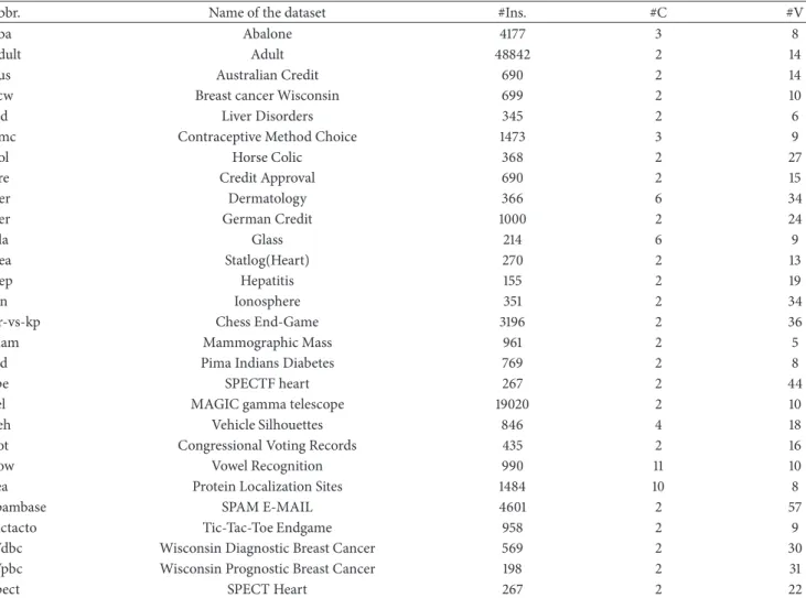
Table 1: List of 28 datasets from UCI Machine Learning Repository and their brief descriptions.
Abbr. Name of the dataset #Ins. #C #V
Aba Abalone 4177 3 8
Adult Adult 48842 2 14
Aus Australian Credit 690 2 14
Bcw Breast cancer Wisconsin 699 2 10
Bld Liver Disorders 345 2 6
Cmc Contraceptive Method Choice 1473 3 9
Col Horse Colic 368 2 27
Cre Credit Approval 690 2 15
Der Dermatology 366 6 34
Ger German Credit 1000 2 24
Gla Glass 214 6 9
Hea Statlog(Heart) 270 2 13
Hep Hepatitis 155 2 19
Ion Ionosphere 351 2 34
Kr-vs-kp Chess End-Game 3196 2 36
Mam Mammographic Mass 961 2 5
Pid Pima Indians Diabetes 769 2 8
Spe SPECTF heart 267 2 44
Tel MAGIC gamma telescope 19020 2 10
Veh Vehicle Silhouettes 846 4 18
Vot Congressional Voting Records 435 2 16
Vow Vowel Recognition 990 11 10
Yea Protein Localization Sites 1484 10 8
Spambase SPAM E-MAIL 4601 2 57
Tictacto Tic-Tac-Toe Endgame 958 2 9
Wdbc Wisconsin Diagnostic Breast Cancer 569 2 30
Wpbc Wisconsin Prognostic Breast Cancer 198 2 31
Spect SPECT Heart 267 2 22
Note. #Ins., #C, and #V mean the number of instances, the number of classes, and the number of variables for the dataset, respectively.
Input:𝐷-training set,{𝐷𝑖}- subsets sampled from𝐷,{𝑚𝑖}- a set of base models,𝐸𝑆- number of base models
or subsets,𝑥-feature vector representing a test sample
Output:𝑅𝑀-a reduced set of base models,𝑃𝐵- a pruned bagging ensemble
1 Collect the subsets of out-of-bag samples as𝑂𝐵𝑖= 𝐷 − 𝐷𝑖, 𝑖 = 1, 2, .., 𝑚𝑎𝑥𝑖𝑡𝑒𝑟.
2 Calculate the center of each𝑂𝐵𝑖as𝐶𝑖,𝑖 = 1, 2, .., 𝑚𝑎𝑥𝑖𝑡𝑒𝑟
3 Calculate the Euclidean distance𝑑𝑖= ‖𝑥 − 𝐶𝑖‖from the test sample𝑥to each center of𝑂𝐵𝑖, 𝑖 = 1, 2, . . . , 𝐸𝑆.
4 Given a parameter𝑡𝑑 ∈ {1, 2, . . . , 10}, compute the threshold𝑇, which is the td-thdecile value of the set
𝐷𝐼𝑆 = {𝑑𝑖| 𝑖 = 1, 2, .., 𝐸𝑆}
5 Initialize𝑅𝑀 = 0.
6 for𝑖 ∈ {1, 2, . . . , 𝐸𝑆}do:
7 if𝑑𝑖≤ 𝑇:
8 𝑅𝑀 = 𝑅𝑀 ∪{𝑚𝑖}
9 The outcome𝑃𝐵(𝑥)of a test sample𝑥predicted by the pruned ensemble𝑃𝐵is given as follows:
𝑃𝐵(𝑥) =majority class in{𝑏𝑚(𝑥) | 𝑏𝑚 ∈ 𝑅𝑀}
Algorithm 3: Distance based pruning for bagging algorithm.
described in Algorithms 4 and 5, respectively. Additionally, the number of base models in the reduced set𝑅𝑀generated by the first stage whatever it is AP or DP was denoted by𝑃, and the corresponding index set of the base models in𝑅𝑀 with respect to the original set was named as{𝑖1, 𝑖2, . . . , 𝑖𝑃} = {𝑖 | 𝑚𝑖∈ 𝑅𝑀}.
4. Analysis of Experimental Results
In order to evaluate the proposed bagging pruning methods, including AP, DP, “AP+DP”, and “DP+AP” procedures, we collected 28 real datasets from UCI Machine Learning Repository [35] to implement the computational experiments
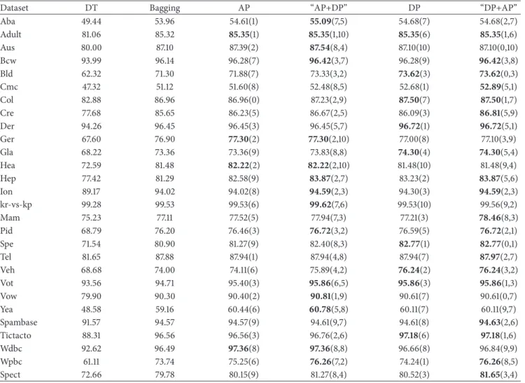
Table 2: Comparison of the classification performance on the 28 datasets between the single classifier DT, bagging using DT as the base learner, and the proposed corresponding pruning methods including AP, DP, “AP+DP” and “DP+AP”. The values in parentheses represent
the optimized parameterstafor AP,tdfor DP, and(ta,td)for “AP+DP” and “DP+AP” with the best classification performance achieved by
the corresponding pruning method.
Dataset DT Bagging AP “AP+DP” DP “DP+AP”
Aba 49.44 53.96 54.61(1) 55.09(7,5) 54.68(7) 54.68(2,7) Adult 81.06 85.32 85.35(1) 85.35(1,10) 85.35(6) 85.35(1,6) Aus 80.00 87.10 87.39(2) 87.54(8,4) 87.10(10) 87.10(0,10) Bcw 93.99 96.14 96.28(7) 96.42(3,7) 96.28(9) 96.42(3,8) Bld 62.32 71.30 71.88(7) 73.33(3,2) 73.62(3) 73.62(0,3) Cmc 47.32 51.12 51.60(8) 52.48(8,5) 52.68(1) 52.89(5,1) Col 82.88 86.96 86.96(0) 87.23(2,9) 87.50(7) 87.50(1,7) Cre 77.68 85.65 86.23(5) 86.67(2,5) 86.09(3) 86.81(5,9) Der 94.26 96.45 96.45(3) 96.45(5,7) 96.72(1) 96.72(5,1) Ger 67.60 76.90 77.30(2) 77.30(2,10) 77.00(8) 77.10(3,9) Gla 68.22 73.36 73.36(9) 73.83(8,8) 74.30(4) 74.30(5,4) Hea 72.59 81.48 82.22(2) 82.22(2,10) 81.48(10) 81.48(9,4) Hep 77.42 81.29 82.58(9) 83.87(2,7) 83.23(2) 83.87(5,6) Ion 89.17 94.02 94.02(8) 94.59(2,3) 94.30(3) 94.59(2,3) kr-vs-kp 99.28 99.53 99.53(6) 99.62(7,6) 99.53(10) 99.56(9,2) Mam 75.23 77.11 77.52(5) 77.94(7,3) 77.21(3) 78.46(8,3) Pid 68.79 76.20 76.46(3) 76.72(3,2) 76.59(5) 76.72(2,1) Spe 71.54 80.90 81.27(9) 82.40(8,3) 82.77(1) 82.77(0,1) Tel 81.65 87.88 87.94(1) 87.94(4,8) 87.94(7) 87.97(2,7) Veh 68.68 74.00 74.11(6) 75.89(4,2) 76.24(2) 76.24(3,2) Vot 93.56 94.71 95.40(3) 95.86(6,5) 95.86(3) 95.86(1,3) Vow 79.90 90.30 90.40(2) 90.81(1,9) 90.61(7) 90.61(0,7) Yea 48.58 59.16 60.44(6) 60.78(5,8) 60.11(7) 60.11(9,7) Spambase 91.57 94.57 94.57(9) 94.61(9,7) 94.61(8) 94.63(2,6) Tictacto 88.31 96.56 96.56(3) 96.76(2,6) 97.18(6) 97.18(1,6) Wdbc 92.62 96.49 97.36(8) 97.36(8,8) 96.66(8) 96.84(9,9) Wpbc 61.11 73.74 75.25(6) 76.26(7,2) 74.24(1) 76.26(8,5) Spect 72.66 79.78 80.15(9) 81.27(8,4) 80.52(3) 81.65(3,4)
by performing and comparing four types of base classifiers. These datasets are listed in Table 1 with brief descriptions about their names, the numbers of instances, classes, and variables (features). The four types of base classifiers include decision tree (DT), Gaussian naive Bayes (GNB), K-nearest neighbors (KNN), and logistic regression (LR), which have been already implemented in the machine learning platform, called scikit-learn [36]. In addition, we adopted fivefold cross validation on any dataset for the proposed pruning methods. For the sake of the simplicity and the consistency, we set the original ensemble size 𝐸𝑆 equal to 200 in the tradi-tional bagging algorithm; i.e., 200 subsets were randomly generated from the training dataset using bootstrap sampling strategy.
4.1. Optimization of AP and DP Procedures. The parameter 𝑡𝑎or𝑡𝑑 with the highest accuracy may be varied with the corresponding dataset. On each dataset, we adopted grid search to optimize the parameters𝑡𝑎and𝑡𝑑of AP and DP procedures, respectively. The value of𝑡𝑎in the AP procedure is ranged from 0 to 9 with step size of 1, and the parameter
𝑡𝑑in the DP procedure is taken to be an integer from 1 to 10 with step size of 1. All possible values of the parameter𝑡𝑎and 𝑡𝑑were examined with paying special attentions to cases in which the accuracy values were achieved by the best.
In AP or DP procedure, given a base classifier on the same dataset, different parameter𝑡𝑎(𝑡𝑎 ∈ {0, 1, 2, 3, 4, 5, 6, 7, 8, 9}) or𝑡𝑑(𝑡𝑑 ∈ {1, 2, 3, 4, 5, 6, 7, 8, 9, 10}) may result in different ensemble size as well as different accuracy value. For a given base classifier, we examined the value of parameter𝑡𝑎or𝑡𝑑 when the accuracy value was achieved by the highest. As shown in Figure 2 for a given 𝑡𝑎and Figure 3 for a given 𝑡𝑑, we counted the number of datasets where the accuracy values were achieved by the best in AP and DP procedures, respectively.
It can be observed that the AP procedure behaved the best in the case of the parameter𝑡𝑎equal to 9. Specially, for a parameter𝑡𝑎of 9, there are 5, 21, 7, and 14 datasets that the best classification can be achieved when the types of the base classifiers are DT, GNB, KNN, and LR, respectively. For any integer𝑡𝑎less than 9, the corresponding amounts of datasets on which the accuracy values are achieved by the highest were
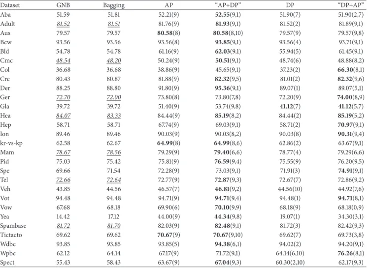
Table 3: Comparison of the classification performance on 28 datasets between the single classifier GNB, bagging using GNB as the base learner, and the proposed corresponding pruning methods including AP, DP, “AP+DP”, and “DP+AP”. The values in parentheses represent
the optimized parameterstafor AP,tdfor DP, and(ta,td)for “AP+DP” and “DP+AP” with the best classification performance achieved by
the corresponding pruning method.
Dataset GNB Bagging AP “AP+DP” DP “DP+AP”
Aba 51.59 51.81 52.21(9) 52.55(9,1) 51.90(7) 51.90(2,7) Adult 81.52 81.51 81.76(9) 81.93(9,1) 81.52(2) 81.89(9,1) Aus 79.57 79.57 80.58(8) 80.58(8,10) 79.57(9) 79.57(9,8) Bcw 93.56 93.56 93.56(8) 93.85(9,1) 93.56(4) 93.71(9,1) Bld 54.78 54.78 61.16(9) 62.03(9,1) 55.94(5) 61.45(9,1) Cmc 48.54 48.20 50.24(9) 50.51(9,1) 48.74(6) 48.88(8,2) Col 36.68 36.68 38.86(9) 45.65(9,1) 37.23(2) 66.30(8,1) Cre 80.43 80.87 81.88(9) 82.32(9,5) 81.01(2) 82.32(9,6) Der 88.25 88.80 91.80(9) 95.36(9,1) 89.07(1) 89.07(5,1) Ger 72.70 72.00 73.80(8) 73.80(7,8) 72.20(9) 74.00(8,9) Gla 39.72 39.72 51.40(9) 53.74(9,8) 41.12(7) 41.12(5,7) Hea 84.07 83.33 84.44(9) 85.19(8,2) 84.44(2) 85.19(5,2) Hep 58.71 58.71 67.74(9) 69.03(9,1) 58.71(2) 70.97(9,1) Ion 89.46 89.46 90.03(9) 90.03(8,2) 90.03(8) 90.31(9,4) kr-vs-kp 62.58 62.67 64.99(8) 64.99(8,6) 62.86(2) 63.67(9,1) Mam 78.67 78.56 79.29(9) 79.40(6,6) 78.77(4) 79.29(6,6) Pid 75.03 75.42 75.81(9) 76.59(9,4) 75.55(9) 76.20(9,5) Spe 69.66 71.54 72.28(9) 73.03(9,1) 71.91(3) 74.91(9,1) Tel 72.66 72.64 72.77(9) 72.87(9,3) 72.67(7) 72.86(9,2) Veh 43.85 44.56 46.57(7) 46.81(9,2) 44.56(10) 44.92(7,6) Vot 94.48 94.48 94.71(9) 94.71(9,4) 94.48(1) 94.71(8,1) Vow 67.68 68.18 69.90(6) 70.10(9,9) 68.18(9) 68.18(0,9) Yea 14.42 17.12 44.00(9) 44.34(9,8) 19.07(1) 34.30(3,1) Spambase 81.72 81.70 82.03(9) 82.48(9,1) 81.72(3) 82.42(9,3) Tictacto 69.62 69.62 70.67(9) 70.67(9,10) 69.62(7) 69.73(3,8) Wdbc 93.85 93.85 93.85(5) 94.38(6,1) 94.02(2) 94.20(9,1) Wpbc 62.12 64.14 67.17(9) 71.72(9,1) 64.14(6,10) 76.26(8,1) Spect 55.43 58.43 63.67(9) 67.04(9,3) 60.30(2,10) 62.17(9,3) 0 1 2 3 4 5 6 7 8 9 ta AP pruning 0 5 10 15 20 25 n u m b er o f da ta sets DT GNB KNN LR
Figure 2: The distribution of the number of datasets with varying parameter ta when the accuracy values were achieved by the highest in the AP procedure.
all smaller than those of cases with𝑡𝑎equal to 9. When the parameter𝑡𝑎is set to be 9, it means that 90% of all base models
in the traditional bagging algorithm will be trimmed off. The empirical results implied that the accuracy-based pruning (AP) method tended to be able to reduce the ensemble size by a large amount, especially for the GNB and LR classifiers. Therefore, we can conclude that the AP pruning under any type of the four base classifiers is an efficient method to reduce the ensemble size of the traditional bagging.
Similarly, we also counted the number of the datasets with the varying parameter𝑡𝑑where the accuracy values reached the highest for the DP procedure. In general, the classification performance was achieved by the best at a different parameter 𝑡𝑑for different dataset, and four base classifiers including DT, GNB, KNN, and LR showed distinct distributions about the numbers of datasets on which the DP procedure performed by the best. As can be observed from Figure 3, when the base classifier type is DT and𝑡𝑑is set to be 3, there are 6 datasets on which the classification performed the best; when the base classifier type is GNB and𝑡𝑑equals 2, the best classification can be achieved based on 9 datasets; when using KNN and 𝑡𝑑to be 2 or 6, seven datasets were found on which the DP
Table 4: Comparison of the classification performance on the 28 datasets between the single classifier KNN, bagging using KNN as the base learner, and the proposed corresponding pruning methods including AP, DP, “AP+DP”, and “DP+AP”. The values in parentheses represent
the optimized parameterstafor AP,tdfor DP, and(ta,td)for “AP+DP” and “DP+AP” with the best classification performance achieved by
the corresponding pruning method.
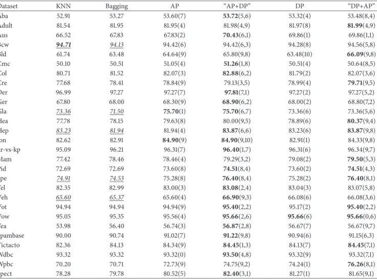
Dataset KNN Bagging AP “AP+DP” DP “DP+AP”
Aba 52.91 53.27 53.60(7) 53.72(5,6) 53.32(4) 53.48(8,4) Adult 81.54 81.95 81.95(4) 81.98(4,9) 81.97(8) 81.99(4,9) Aus 66.52 67.83 67.83(2) 70.43(6,1) 69.86(1) 69.86(1,1) Bcw 94.71 94.13 94.42(6) 94.42(6,3) 94.28(8) 94.56(5,8) Bld 61.74 63.48 64.64(9) 65.80(9,8) 63.48(10) 66.09(9,8) Cmc 50.10 50.51 51.05(4) 51.26(1,8) 50.51(4) 50.64(8,5) Col 80.71 81.52 82.07(3) 82.88(6,2) 81.79(2) 82.07(3,6) Cre 77.68 78.41 78.84(9) 79.13(3,5) 78.99(4) 79.71(9,5) Der 96.99 97.27 97.27(7) 97.81(7,1) 97.27(2) 97.27(5,2) Ger 67.80 68.00 68.30(9) 68.90(6,2) 68.00(2) 68.80(7,2) Gla 73.36 71.50 75.70(1) 75.70(6,7) 73.36(6) 73.36(5,6) Hea 77.78 78.15 79.63(8) 80.00(9,5) 78.89(6) 80.37(9,4) Hep 83.23 81.94 81.94(4) 83.87(6,6) 83.23(6) 83.87(9,8) Ion 82.62 82.91 84.90(9) 84.90(9,10) 82.91(1) 84.33(9,8) kr-vs-kp 95.09 96.21 96.31(7) 96.40(1,7) 96.31(6) 96.34(9,7) Mam 77.42 78.46 78.46(4) 79.29(3,2) 79.08(2) 79.50(5,3) Pid 72.69 72.69 73.60(8) 74.51(8,4) 73.60(2) 74.51(4,3) Spe 74.91 74.53 75.28(8) 76.40(8,4) 75.28(2) 76.40(8,1) Tel 82.35 82.99 83.00(3) 83.08(2,4) 83.04(3) 83.07(5,8) Veh 65.60 65.37 65.60(4) 66.90(9,3) 66.08(6) 66.08(3,6) Vot 94.94 94.94 94.94(9) 95.40(2,2) 95.17(2) 95.40(2,2) Vow 95.05 95.35 95.56(4) 95.66(2,6) 95.66(6) 95.66(0,6) Yea 53.98 56.40 56.74(3) 56.87(2,8) 56.67(7) 56.67(9,7) Spambase 90.00 90.74 91.02(7) 91.22(9,8) 90.94(6) 91.15(6,3) Tictacto 82.36 84.13 84.34(9) 84.45(1,3) 84.13(7) 84.45(7,1) Wdbc 93.32 93.32 93.32(0) 93.50(4,8) 93.32(9) 93.32(7,1) Wpbc 70.20 70.71 72.73(9) 74.75(9,2) 74.24(1) 76.26(8,1) Spect 78.28 79.78 80.52(5) 82.40(3,1) 81.27(1) 81.65(9,1) 1 2 3 4 5 6 7 8 9 10 td DP pruning DT GNB KNN LR 0 2 4 6 8 10 n u m b er o f da ta sets
Figure 3: The distribution of the number of datasets with varying
parametertdwhen the accuracy values were achieved by the highest
in the DP procedure.
procedure can perform the best; when the base learner LR is adopted and the parameter𝑡𝑑is set to be 2, we observed that the best classification can be achieved on 6 datasets. The
numbers of datasets counted in all cases mentioned above for a given parameter𝑡𝑑are the largest when compared with those counted for other possible values of the parameter td. In the DP procedure, much more number of base classifiers will be excluded if smaller parameter 𝑡𝑑 is taken. The empirical results showed that this DP pruning method tends to reduce the ensemble size by a large amount, although it is not so much significant when compared with the AP procedure.
4.2. Result Analysis for Two-Stage Pruning Methods. As mentioned above, we further combined the AP and DP procedures that generated two strategies for two-stage pruning and examined their classification performance by
varying the parameters 𝑡𝑎 of AP and 𝑡𝑑 of DP based
on 28 datasets. The first two-stage pruning method is “AP+DP”. The computational experiments were carried out according to Algorithm 4 by simultaneously varying 𝑡𝑎 ∈ {0, 1, 2, 3, 4, 5, 6, 7, 8, 9} and 𝑡𝑑 ∈ {1, 2, 3, 4, 5, 6, 7, 8, 9, 10}. We also counted the numbers of datasets on which the classification performance measured using accuracy value
DT GNB KNN LR 1 2 3 4 11 2 4 6 8 0 10 ta 10 8 6 4 td 2 0 2 4 6 8 0 10 ta 10 8 6 4 td 2 0 2 4 6 8 0 10 ta 10 8 6 4 td 2 0 2 4 6 8 0 10 ta 10 8 6 4 td 2 0
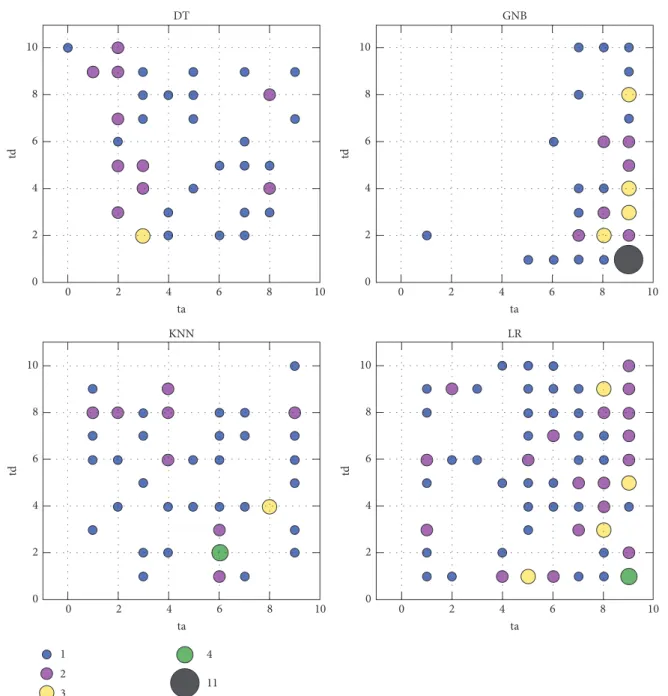
Figure 4: The distributions of the numbers of datasets with varyingtaandtdwhen the classification performance was achieved by the best
for “AP+DP” pruning. The number of datasets corresponding to a pair oftaandtdis represented as the size of a colored solid circle. The
types of all solid circles and their corresponding values are listed at the bottom of the figure.
was optimized with the varying parameters𝑡𝑎and 𝑡𝑑. The distributions for four different base classifiers (i.e., DT, GNB, KNN, and LR) were shown in Figure 4, where the number of datasets corresponding to certain pair of𝑡𝑎and td was represented as the size of a colored circle, each color meaning a positive integer. It can be easily found that GNB tends to be the most efficient base classifier for reducing the ensemble size when compared with other three base classifiers (DT, KNN, and LR). Specially, given GNB as the base classifier, it is somewhat surprising that there are 11 out of 28 datasets on which the accuracy was achieved by the best with the parameters𝑡𝑎 = 9 and𝑡𝑑 = 1. In these cases, 90% of the
base models were excluded by the AP procedure and further 90% of the reduced set of base models of AP were trimmed off after the DP stage. The second efficient one on reducing the ensemble size is LR, since majority of datasets were counted at the parameters𝑡𝑎 ∈ {5, 6, 7, 8, 9}and𝑡𝑑 ∈ {1, 2, .., 7}. Other two types of classifiers DT and KNN showed relatively weaker ability to reduce the original ensemble size, since they held much more diverse distribution of the numbers of datasets with varying parameter𝑡𝑎and𝑡𝑑.
The second two-stage pruning experiment is “DP+AP” performed in terms of Algorithm 5. Similarly as the first two-stage method “AP+DP”, the distributions of the numbers
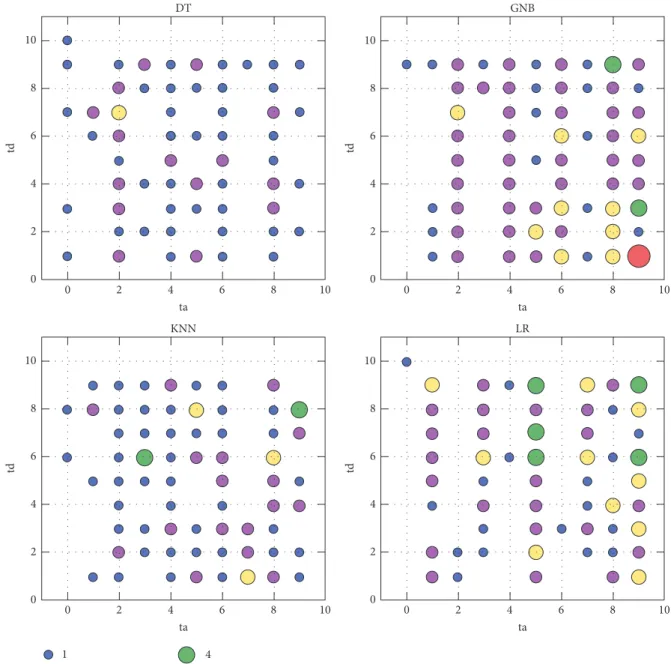
1 2 3 4 7 DT GNB KNN LR 2 4 6 8 0 10 ta 10 8 6 4 td 2 0 2 4 6 8 0 10 ta 10 8 6 4 td 2 0 2 4 6 8 0 10 ta 10 8 6 4 td 2 0 2 4 6 8 0 10 ta 10 8 6 4 td 2 0
Figure 5: The distributions of the numbers of datasets with the varying parameterstaandtdwhen the classification performance was achieved
by the best for “DP+AP” pruning. The number of datasets corresponding to a pair oftaandtdis represented as the size of a colored solid
circle. The types of all solid circles and their corresponding values are listed at the bottom of the red.
of datasets with varying parameters𝑡𝑑and𝑡𝑎for four base classifiers when the classification performance was optimized were plotted as shown in Figure 5. The distributions generated by “DP+AP” pruning method are relatively more diverse for all cases of the four base classifiers when compared with the “AP+DP”. However, it is consistent that GNB exhibited the most apparent tend to the ability to reduce the ensemble size by a large amount. As a result, both “AP+DP” and “DP+AP” are generally effective in reducing the size of the original ensemble, although these two methods showed distinct ability to the extent to the ensemble size reduction.
4.3. Performance Comparison among Single Base Classifier, Bagging, and the Proposed Pruning Methods. We compared the experimental results performed by a single classifier, the corresponding bagging, and the proposed pruning methods including AP, DP, “AP+DP”, and “DP+AP”. The accuracy values based on fivefold cross validation were calculated based on 28 datasets and listed in Tables 2, 3, 4, and 5 for DT, GNB, KNN, and LR, respectively. For the pruning methods including AP, DP, “AP+DP”, and “DP+AP”, we only reported the accuracy values together with the optimized parameters 𝑡𝑎and𝑡𝑑, which were listed in parentheses. In addition, the highest accuracy value among the single classifier, bagging,
Table 5: Comparison of the classification performance on the 28 datasets between the single classifier LR, bagging using LR as the base learner, and the proposed corresponding pruning methods including AP, DP, “AP+DP”, and “DP+AP”. The values in parentheses represent
the optimized parameterstafor AP,tdfor DP, and(ta,td)for “AP+DP” and “DP+AP” with the best classification performance achieved by
the corresponding pruning method.
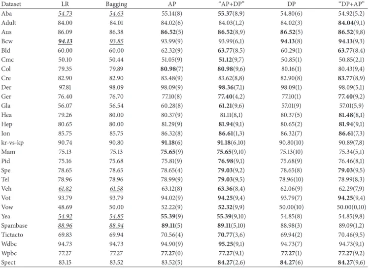
Dataset LR Bagging AP “AP+DP” DP “DP+AP”
Aba 54.73 54.63 55.14(8) 55.37(8,9) 54.80(6) 54.92(5,2) Adult 84.00 84.01 84.02(6) 84.03(1,2) 84.02(3) 84.04(9,1) Aus 86.09 86.38 86.52(5) 86.52(8,9) 86.52(5) 86.52(9,8) Bcw 94.13 93.85 93.99(9) 93.99(6,1) 94.13(8) 94.13(9,3) Bld 60.00 60.00 62.32(9) 63.77(8,5) 60.29(1) 63.77(8,4) Cmc 50.10 50.44 51.05(9) 51.12(9,7) 50.85(1) 50.85(2,1) Col 79.35 79.89 80.98(7) 80.98(9,6) 80.16(1) 80.43(9,4) Cre 82.90 82.90 83.48(9) 83.62(8,8) 82.90(8) 83.77(8,9) Der 97.81 98.09 98.09(9) 98.36(7,1) 98.09(1) 98.09(5,1) Ger 76.40 76.70 77.10(8) 77.40(4,2) 77.10(1) 77.40(9,2) Gla 56.07 56.54 60.28(8) 61.21(9,6) 57.01(9) 57.01(5,9) Hea 79.26 80.00 80.37(9) 81.11(8,1) 80.37(5) 81.48(8,1) Hep 80.65 80.00 81.29(9) 81.94(9,1) 80.65(2) 81.94(9,1) Ion 85.75 85.75 86.32(8) 86.61(1,3) 86.32(7) 86.61(7,3) kr-vs-kp 90.74 90.80 91.18(6) 91.18(6,10) 90.80(10) 90.89(7,8) Mam 75.13 75.13 75.65(9) 75.65(9,10) 75.13(10) 75.34(5,1) Pid 75.16 75.68 75.81(9) 76.98(9,1) 75.68(9) 76.46(8,1) Spe 78.65 78.65 78.65(4) 79.03(9,2) 78.65(8) 79.03(9,5) Tel 78.96 78.96 78.99(9) 79.03(9,5) 78.96(10) 78.99(8,3) Veh 61.82 61.58 63.12(8) 63.36(8,4) 62.06(9) 62.29(7,9) Vot 93.79 93.79 94.02(9) 94.25(9,4) 93.79(7) 94.25(9,4) Vow 48.69 50.00 52.22(9) 52.32(9,9) 50.00(10) 50.00(0,10) Yea 54.92 54.85 55.39(9) 55.39(9,10) 54.85(8) 54.85(9,8) Spambase 88.96 88.94 89.11(5) 89.11(5,10) 88.98(3) 89.09(1,2) Tictacto 69.83 69.94 70.56(4) 70.77(3,6) 69.94(2) 70.46(9,5) Wdbc 94.73 94.73 94.90(9) 95.25(9,1) 94.73(7) 94.73(9,1) Wpbc 77.27 77.27 77.27(0) 77.27(9,1) 77.27(1) 77.27(9,2) Spect 83.15 83.52 83.52(5) 84.27(2,6) 84.27(6) 84.27(9,6)
Input:𝑅𝑀-a reduced set of base models generated by the AP procedure,𝑃- number of base models in𝑅𝑀,
{𝑖1, 𝑖2, . . . , 𝑖𝑃}- index set of base models in𝑅𝑀,𝑥-feature vector of a test sample
Output:𝑅𝑀2-a reduced set of base models,𝑃𝐵2- a pruned bagging ensemble
1 Given a parameter𝑡𝑑 ∈ {1, 2, . . . , 10}, compute the threshold𝑇, which is the td-th decile value of the set
𝐷𝐼𝑆 = {𝑑𝑘 | 𝑘 ∈ {𝑖1, 𝑖2, . . . , 𝑖𝑃}}.
2 Initialize𝑅𝑀2 = 0.
3 for𝑘 ∈ {𝑖1, 𝑖2, . . . , 𝑖𝑃}do:
4 if𝑑𝑘≤ 𝑇:
5 𝑅𝑀2 = 𝑅𝑀2 ∪{𝑚𝑘}
6 The outcome𝑃𝐵2(𝑥)of a test sample𝑥predicted by the pruned ensemble𝑃𝐵2is given as follows:
𝑃𝐵2(𝑥) =majority class in{𝑏𝑚(𝑥) | 𝑏𝑚 ∈ 𝑅𝑀2}
Algorithm 4: Two-stage pruning for “AP+DP”.
and the proposed pruning methods on each dataset was highlighted using bold font.
In general, the traditional bagging performed better than the corresponding single classifier. However, sometimes, there is no improvement even decrease on classification performance when comparing bagging with the underlying
single classifier. For example, as shown in Table 3, the accuracy value of bagging using GNB as the base classifier on the Ger dataset is 72.00%, which is lower than that of the single GNB classifier equal to 72.70%. Such cases are marked with underlined italic fonts in Tables 2–5. Several authors, e.g., Dietterich [6] and Croux et al. [26], also pointed out
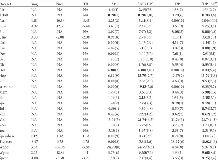
Table 6: Relative improvement of the proposed bagging pruning methods and existing other three variations with respect to the traditional
bagging using DT as the base classifier. The values in parentheses represent the optimized parameterstafor AP,tdfor DP, and(ta,td)for
“AP+DP” and “DP+AP” with the best classification performance achieved by the corresponding pruning method.
Dataset Brag Nice TB AP “AP+DP” DP “DP+AP”
Aba NA NA NA 1.41(1) 2.45(7,5) 1.56(7) 1.56(2,7) Adult NA NA NA 0.20(1) 0.20(1,10) 0.20(6) 0.20(1,6) Aus 1.15 -10.34 -3.45 2.25(2) 3.41(8,4) 0.00(10) 0.00(0,10) Bcw -1.37 -12.33 -5.48 3.63(7) 7.25(3,7) 3.63(9) 7.25(3,8) Bld NA NA NA 2.02(7) 7.07(3,2) 8.08(3) 8.08(0,3) Cmc 0.00 -2.08 -2.08 0.98(8) 2.78(8,5) 3.19(1) 3.62(5,1) Col NA NA NA 0.00(0) 2.07(2,9) 4.14(7) 4.14(1,7) Cre NA NA NA 4.04(5) 7.11(2,5) 3.07(3) 8.08(5,9) Der NA NA NA 0.00(3) 0.00(5,7) 7.61(1) 7.61(5,1) Ger NA NA NA 1.73(2) 1.73(2,10) 0.43(8) 0.87(3,9) Gla NA NA NA 0.00(9) 1.76(8,8) 3.53(4) 3.53(5,4) Hea NA NA NA 4.00(2) 4.00(2,10) 0.00(10) 0.00(9,4) Hep NA NA NA 6.89(9) 13.79(2,7) 10.37(2) 13.79(5,6) Ion NA NA NA 0.00(8) 9.53(2,3) 4.68(3) 9.53(2,3) kr-vs-kp NA NA NA 0.00(6) 19.15(7,6) 0.00(10) 6.38(9,2) Mam NA NA NA 1.79(5) 3.63(7,3) 0.44(3) 5.90(8,3) Pid NA NA NA 1.09(3) 2.18(3,2) 1.64(5) 2.18(2,1) Spe NA NA NA 1.94(9) 7.85(8,3) 9.79(1) 9.79(0,1) Tel NA NA NA 0.50(1) 0.50(4,8) 0.50(7) 0.74(2,7) Veh NA NA NA 0.42(6) 7.27(4,2) 8.62(2) 8.62(3,2) Vot NA NA NA 13.04(3) 21.74(6,5) 21.74(3) 21.74(1,3) Vow NA NA NA 1.03(2) 5.26(1,9) 3.20(7) 3.20(0,7) Yea NA NA NA 3.13(6) 3.97(5,8) 2.33(7) 2.33(9,7) Spambase 1.12 1.12 1.12 0.00(9) 0.74(9,7) 0.74(8) 1.10(2,6) Tictacto -8.47 6.78 6.78 0.00(3) 5.81(2,6) 18.02(6) 18.02(1,6) Wdbc 3.53 -67.06 -5.88 24.79(8) 24.79(8,8) 4.84(8) 9.97(9,9) Wpbc 2.22 -18.89 1.11 5.75(6) 9.60(7,2) 1.90(1) 9.60(8,5) Spect -1.08 -5.38 -3.23 1.83(9) 7.37(8,4) 3.66(3) 9.25(3,4)
Note.“NA” means not available.
Input:𝑅𝑀-a reduced set of base models generated by DP procedure for a specific test sample𝑥,𝑃- number of
base models in𝑅𝑀,{𝑖1, 𝑖2, . . . , 𝑖𝑃}- index set of base models in𝑅𝑀
Output:𝑅𝑀2-a reduced set of base models,𝑃𝐵2- a pruned bagging ensemble
1 Given a parameter ta∈ {0, 1, 2, . . . , 9}, compute the threshold𝑇, which is the ta-th decile value of the set
{𝐴𝐶𝑘| 𝑘 ∈ {𝑖1, 𝑖2, . . . , 𝑖𝑃}}.
2 Initialize𝑅𝑀2 = 0.
3 for𝑘 ∈ {𝑖1, 𝑖2, . . . , 𝑖𝑃}do:
4 if𝐴𝐶𝑘≥ 𝑇:
5 𝑅𝑀2 = 𝑅𝑀2 ∪{𝑚𝑘}
6 The outcome𝑃𝐵2(𝑥)of a test sample𝑥predicted by the pruned ensemble𝑃𝐵2is given as follows:
𝑃𝐵2(𝑥) =majority class in{𝑏𝑚(𝑥) | 𝑏𝑚 ∈ 𝑅𝑀2}
Algorithm 5: Two-stage pruning for “DP+AP”.
that there was no guarantee that bagging will improve the performance of any base classifier. Nevertheless, there is at least one of the proposed pruning methods that performed better than both the single classifier and the bagging for such cases. This implied that our proposed pruning methods were effective on all 28 datasets.
As shown in Tables 2–5, for the base classifiers DT, GNB, KNN, and LR, there are, respectively, 20, 26, 21, and 24 (71.43%,92.86%,75%, and 85.71%) out of 28 datasets on which the classification performance of the single AP stage was increased when compared with the traditional bagging. The accuracy value of AP pruning was increased by 0.39%, 3.05%,
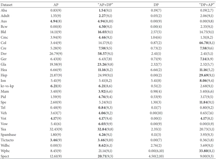
Table 7: Relative improvement of the proposed bagging pruning methods with respect to the traditional bagging using GNB as the base
classifier. The values in parentheses represent the optimized parameterstafor AP,tdfor DP, and(ta,td)for “AP+DP” and “DP+AP” with the
best classification performance achieved by the corresponding pruning method.
Dataset AP “AP+DP” DP “DP+AP”
Aba 0.83(9) 1.54(9,1) 0.19(7) 0.19(2,7) Adult 1.35(9) 2.27(9,1) 0.05(2) 2.06(9,1) Aus 4.94(8) 4.94(8,10) 0.00(9) 0.00(9,8) Bcw 0.00(8) 4.50(9,1) 0.00(4) 2.33(9,1) Bld 14.11(9) 16.03(9,1) 2.57(5) 14.75(9,1) Cmc 3.94(9) 4.46(9,1) 1.04(6) 1.31(8,2) Col 3.44(9) 14.17(9,1) 0.87(2) 46.78(8,1) Cre 5.28(9) 7.58(9,5) 0.73(2) 7.58(9,6) Der 26.79(9) 58.57(9,1) 2.41(1) 2.41(5,1) Ger 6.43(8) 6.43(7,8) 0.71(9) 7.14(8,9) Gla 19.38(9) 23.26(9,8) 2.32(7) 2.32(5,7) Hea 6.66(9) 11.16(8,2) 6.66(2) 11.16(5,2) Hep 21.87(9) 24.99(9,1) 0.00(2) 29.69(9,1) Ion 5.41(9) 5.41(8,2) 5.41(8) 8.06(9,4) kr-vs-kp 6.21(8) 6.21(8,6) 0.51(2) 2.68(9,1) Mam 3.40(9) 3.92(6,6) 0.98(4) 3.40(6,6) Pid 1.59(9) 4.76(9,4) 0.53(9) 3.17(9,5) Spe 2.60(9) 5.24(9,1) 1.30(3) 11.84(9,1) Tel 0.48(9) 0.84(9,3) 0.11(7) 0.80(9,2) Veh 3.63(7) 4.06(9,2) 0.00(10) 0.65(7,6) Vot 4.17(9) 4.17(9,4) 0.00(1) 4.17(8,1) Vow 5.41(6) 6.03(9,9) 0.00(9) 0.00(0,9) Yea 32.43(9) 32.84(9,8) 2.35(1) 20.73(3,1) Spambase 1.80(9) 4.26(9,1) 0.11(3) 3.93(9,3) Tictacto 3.46(9) 3.46(9,10) 0.00(7) 0.36(3,8) Wdbc 0.00(5) 8.62(6,1) 2.76(2) 5.69(9,1) Wpbc 8.45(9) 21.14(9,1) 0.00(6,10) 33.80(8,1) Spect 12.61(9) 20.71(9,3) 4.50(2,10) 9.00(9,3)
0.61%, and 0.65% on average over all 28 datasets when the base classifier was DT, GNB, KNN, and LR, respectively. Similarly, the DP procedure can improve the classification performance of the traditional bagging on 25 (89.29%), 20 (71.43%), 21 (75%), and 15 (53.57%) out of the 28 datasets for the base classifiers DT, GNB, KNN, and LR, respectively. Moreover, the accuracy improvement when comparing the DP pruning with the traditional bagging using DT, GNB, KNN, and LR as base classifier is on average 0.65%, 0.39%, 0.58%, and 0.19%, respectively. When comparing AP and DP based on the relative improvement, AP is much more powerful than DP although the improvement in case of DT as the base classifier using AP procedure is relatively lower than that using DP procedure.
Moreover, using AP procedure as the first pruning stage, the two-stage pruning method “AP+DP” resulted in increase of classification accuracy on 27 (96.43%), 28 (100%), 28 (100%), and 27 (96.43%) out of 28 datasets for the base classifiers DT, GNB, KNN, and LR, respectively, when com-pared with the traditional bagging. The average accuracy improvements of the “AP+DP” method with respect to
the traditional bagging using DT, GNB, KNN, and LR are 0.88%, 4.06%,1.26%, and 0.96%, which further improved the classification accuracy values of both AP and DP methods. Moreover, if the first stage is DP, the proposed two-stage pruning approach “DP+AP” gained the improvement of classification performance on 26 (92.86%), 26 (92.86%), 26 (92.86%), and 20 (71.43%) out of 28 datasets for the base clas-sifiers DT, GNB, KNN, and LR, respectively, when compared with the traditional bagging. The corresponding average accuracy improvements are 0.90%, 3.52%, 1.08%, and 0.57%, respectively. In addition, there are 9 (32.14%), 19 (67.86%), 15 (53.57%), and 15 (53.57%) out of 28 datasets on which “AP+DP” performed better than “DP+AP”, and the average accuracy improvements of “AP+DP” when compared with “DP+AP” are -0.01%, 0.54%, 0.17%, and 0.39%, respectively, for DT, GNB, KNN, and LR. As a result, the classification performance of “AP+DP” using DT as the base learner is overall very close to that of “DP+AP”, and “AP+DP” performed better than “DP+AP” on majority of 28 datasets when using other three methods GNB, KNN, and LR as the base classifiers.
Table 8: Relative improvement of the proposed bagging pruning methods with respect to the traditional bagging using KNN as the base
classifier. The values in parentheses represent the optimized parameterstafor AP,tdfor DP, and(ta,td)for “AP+DP” and “DP+AP” with the
best classification performance achieved by the corresponding pruning method.
Dataset AP “AP+DP” DP “DP+AP”
Aba 0.71(7) 0.96(5,6) 0.11(4) 0.45(8,4) Adult 0.00(4) 0.17(4,9) 0.11(8) 0.22(4,9) Aus 0.00(2) 8.08(6,1) 6.31(1) 6.31(1,1) Bcw 4.94(6) 4.94(6,3) 2.56(8) 7.33(5,8) Bld 3.18(9) 6.35(9,8) 0.00(10) 7.15(9,8) Cmc 1.09(4) 1.52(1,8) 0.00(4) 0.26(8,5) Col 2.98(3) 7.36(6,2) 1.46(2) 2.98(3,6) Cre 1.99(9) 3.33(3,5) 2.69(4) 6.02(9,5) Der 0.00(7) 19.78(7,1) 0.00(2) 0.00(5,2) Ger 0.94(9) 2.81(6,2) 0.00(2) 2.50(7,2) Gla 14.74(1) 14.74(6,7) 6.53(6) 6.53(5,6) Hea 6.77(8) 8.47(9,5) 3.39(6) 10.16(9,4) Hep 0.00(4) 10.69(6,6) 7.14(6) 10.69(9,8) Ion 11.64(9) 11.64(9,10) 0.00(1) 8.31(9,8) kr-vs-kp 2.64(7) 5.01(1,7) 2.64(6) 3.43(9,7) Mam 0.00(4) 3.85(3,2) 2.88(2) 4.83(5,3) Pid 3.33(8) 6.66(8,4) 3.33(2) 6.66(4,3) Spe 2.94(8) 7.34(8,4) 2.94(2) 7.34(8,1) Tel 0.06(3) 0.53(2,4) 0.29(3) 0.47(5,8) Veh 0.66(4) 4.42(9,3) 2.05(6) 2.05(3,6) Vot 0.00(9) 9.09(2,2) 4.55(2) 9.09(2,2) Vow 4.52(4) 6.67(2,6) 6.67(6) 6.67(0,6) Yea 0.78(3) 1.08(2,8) 0.62(7) 0.62(9,7) Spambase 3.02(7) 5.18(9,8) 2.16(6) 4.43(6,3) Tictacto 1.32(9) 2.02(1,3) 0.00(7) 2.02(7,1) Wdbc 0.00(0) 2.69(4,8) 0.00(9) 0.00(7,1) Wpbc 6.90(9) 13.79(9,2) 12.05(1) 18.95(8,1) Spect 3.66(5) 12.96(3,1) 7.37(1) 9.25(9,1)
From above, we can conclude that the proposed pruning methods are able to improve the classification performance when compared with the traditional bagging. Furthermore, the two-stage pruning method is much more powerful than the single pruning approach. Although “DP+AP” using DT as the base classifier performed very slightly better than “AP+DP”, it is obvious that the computation performed by “AP+DP” will be much faster than that of “DP+AP”. Therefore, from the view of the current bagging pruning framework, we recommend using “AP+DP” to prune the traditional bagging for reducing the ensemble size and improving the classification performance for base classifiers DT, GNB, KNN, and LR.
4.4. Comparison with Other Existing Bagging Algorithms. We compared the proposed pruning methods with other three variations of the bagging algorithm including Brag (Bootstrap robust aggregating) [37], Nice (Nice Bagging) [25], and TB (Trimmed Bagging) [26]. Brag is actually not a bagging pruning method and calculates the median of the outcomes of all the bootstrapped classifiers instead of computing an average like the traditional bagging. Nice [25]
averaged over the outcomes of the bootstrapped classifiers that performed better than the initial base classifier, while TB [26] excluded the 25% “worse” classifiers and aggregated the rest. Both Nice and TB as well as the AP method presented in this work are bagging pruning methods using a similar rule by excluding “bad” classifiers validated on the out-of-bag samples. The relative improvement of different out-of-bagging variations with respect to the traditional bagging under four base classifiers DT, GNB, KNN, and LR is listed in Tables 6, 7, 8, and 9, respectively. As shown in these tables, we only showed the available results (“NA” means not available as shown in Tables 6 and 9) for Brag, Nice, and TB on 8 datasets where their relative improvement values listed in Tables 6 and 9 were all derived from the work by Croux et al. [26] However, this work [26] did not perform the bagging methods that used GNB or KNN as the base classifier.
From the view of relative improvement, it can be easily found that the proposed two-stage pruning methods, such as “AP+DP” and “DP+AP”, performed overall better than other bagging methods including Brag, Nice, TB, AP, and DP. The difference between “AP+DP” and “DP+AP” is small on average. DP performed slightly better than AP when
Table 9: Relative improvement of the proposed bagging pruning methods and existing other three variations with respect to the traditional
bagging using LR as the base classifier. The values in parentheses represent the optimized parameterstafor AP,tdfor DP, and(ta,td)for
“AP+DP” and “DP+AP” with the best classification performance achieved by the corresponding pruning method.
Dataset Brag Nice TB AP “AP+DP” DP “DP+AP”
Aba NA NA NA 1.12(8) 1.63(8,9) 0.37(6) 0.64(5,2) Adult NA NA NA 0.06(6) 0.13(1,2) 0.06(3) 0.19(9,1) Aus 0.00 -1.00 -1.00 1.03(5) 1.03(8,9) 1.03(5) 1.03(9,8) Bcw 0.00 0.00 -3.23 2.28(9) 2.28(6,1) 4.55(8) 4.55(9,3) Bld NA NA NA 5.80(9) 9.43(8,5) 0.72(1) 9.43(8,4) Cmc 0.00 1.00 0.00 1.23(9) 1.37(9,7) 0.83(1) 0.83(2,1) Col NA NA NA 5.42(7) 5.42(9,6) 1.34(1) 2.69(9,4) Cre NA NA NA 3.39(9) 4.21(8,8) 0.00(8) 5.09(8,9) Der NA NA NA 0.00(9) 14.14(7,1) 0.00(1) 0.00(5,1) Ger NA NA NA 1.72(8) 3.00(4,2) 1.72(1) 3.00(9,2) Gla NA NA NA 8.61(8) 10.75(9,6) 1.08(9) 1.08(5,9) Hea NA NA NA 1.85(9) 5.55(8,1) 1.85(5) 7.40(8,1) Hep NA NA NA 6.45(9) 9.70(9,1) 3.25(2) 9.70(9,1) Ion NA NA NA 4.00(8) 6.04(1,3) 4.00(7) 6.04(7,3) kr-vs-kp NA NA NA 4.13(6) 4.13(6,10) 0.00(10) 0.98(7,8) Mam NA NA NA 2.09(9) 2.09(9,10) 0.00(10) 0.84(5,1) Pid NA NA NA 0.53(9) 5.35(9,1) 0.00(9) 3.21(8,1) Spe NA NA NA 0.00(4) 1.78(9,2) 0.00(8) 1.78(9,5) Tel NA NA NA 0.14(9) 0.33(9,5) 0.00(10) 0.14(8,3) Veh NA NA NA 4.01(8) 4.63(8,4) 1.25(9) 1.85(7,9) Vot NA NA NA 3.70(9) 7.41(9,4) 0.00(7) 7.41(9,4) Vow NA NA NA 4.44(9) 4.64(9,9) 0.00(10) 0.00(0,10) Yea NA NA NA 1.20(9) 1.20(9,10) 0.00(8) 0.00(9,8) Spambase 0.00 8.33 1.04 1.54(5) 1.54(5,10) 0.36(3) 1.36(1,2) Tictacto 0.00 0.00 0.00 2.06(4) 2.76(3,6) 0.00(2) 1.73(9,5) Wdbc 0.00 -23.73 -16.95 3.23(9) 9.87(9,1) 0.00(7) 0.00(9,1) Wpbc 0.00 -15.15 -1.01 0.00(0) 0.00(9,1) 0.00(1) 0.00(9,2) Spect 0.00 -2.35 -7.06 0.00(5) 4.55(2,6) 4.55(6) 4.55(9,6)
Note:“NA” means not available.
using DT as the base classifier. In addition, when the base learner GNB or KNN was applied to the bagging, as shown in Tables 7 and 8 we can conclude that “AP+DP” performed the best, followed by DP+AP, AP, and DP. In the context of the base classifier LR, our proposed two-stage pruning methods performed better than the other three approaches including Brag, Nice, and TB on majority of the 8 datasets. Even, when one of the methods Brag, Nice, and TB performed worse than the traditional bagging (i.e., negative relative improvement), our two-stage pruning methods including “AP+DP” and “DP+AP” can still improve the classification performance when compared with the traditional bagging.
4.5. Comparison of Classification Performance between Dif-ferent Base Classifiers. In this section, we reported the best results according to the types of base classifiers on all datasets. The highest classification accuracy value on each dataset for every base classifier reported in Tables 2–5 was collected into Table 10. The best result for each base learner was represented by the highest classification accuracy among the
proposed pruning methods including AP, DP, “AP+DP”, and “DP+AP”.
On 19 out of 28 (67.86%) datasets, the proposed pruning methods using DT as the base classifier gained the highest classification accuracy compared with other base learners GNB, KNN, and LR. Otherwise, the pruning methods using three base classifiers GNB, KNN, and LR performed by the best on 3.57%, 10.71%, and 21.43% datasets, respectively. From the above experimental results, we recommend that DT of these four base classifiers should be the first choice for pruning the traditional bagging when given data source. However, it cannot be ensured that DT always performs the best on any dataset. GNB, KNN, and LR are also the possible choice.
5. Conclusion
In this work, we proposed two-stage bagging pruning meth-ods that are composed of two simple pruning methmeth-ods called AP and DP. The two-stage bagging methods, “AP+DP” and
Table 10: The highest classification accuracy values on 28 datasets when using four types of base classifiers DT, GNB, KNN, and LR. Dataset DT GNB KNN LR Aba 55.09 52.55 53.72 55.37 Adult 85.35 81.93 81.99 84.04 Aus 87.54 80.58 69.86 86.52 Bcw 96.42 93.85 94.71 94.13 Bld 73.62 62.03 66.09 63.77 Cmc 52.89 50.51 51.26 51.12 Col 87.50 66.30 82.88 80.98 Cre 86.81 82.32 79.71 83.77 Der 96.72 95.36 97.81 98.36 Ger 77.30 74.00 68.90 77.40 Gla 74.30 41.12 75.70 61.21 Hea 82.22 85.19 80.37 81.48 Hep 83.87 70.97 83.87 81.94 Ion 94.59 90.31 84.90 86.61 Kr-vs-kp 99.62 64.99 96.40 91.18 Mam 78.46 79.40 79.50 75.65 Pid 76.72 76.59 74.51 76.98 Spe 82.77 74.91 76.40 79.03 Tel 87.97 72.87 83.08 79.03 Veh 76.24 46.81 66.90 63.36 Vot 95.86 94.71 95.40 94.25 Vow 90.81 70.10 95.66 52.32 Yea 60.78 44.34 56.87 55.39 Spambase 94.63 82.48 91.22 89.11 Tictacto 97.18 70.67 84.45 70.77 Wdbc 97.36 94.38 93.50 95.25 Wpbc 76.26 76.26 76.26 77.27 Spect 81.65 67.04 82.40 84.27
“DP+AP”, are implemented by combining the individual AP and DP in two forms. They outperformed the one-stage methods AP and DP that were evaluated on 28 datasets using four types of base classifiers DT, GNB, KNN, and LR. Overall, the method “AP+DP” performed better than the other one called “DP+AP”. Although the latter behaved very close to or even slightly better than the former when using DT as the base classifier, the computational imple-mentation of “AP+DP” was much faster than “DP+AP”. Therefore, we strongly recommend the two-stage pruning method “AP+DP” as the final pruning approach for any type of base classifiers including DT, GNB, KNN, and LR.
The proposed pruning method given DT as the base classifier usually outperformed ones with other base learn-ers, such as GNB, KNN, and LR, on majority of the 28 datasets. This implied that DT should be the first choice of base classifiers for the proposed bagging pruning methods. In addition, given GNB or LR as the base learner, the two-stage pruning method “AP+DP” can greatly reduce the ensemble size and improve the classification perfor-mance. As a summary, the proposed two-stage pruning methods are promising approaches that can efficiently reduce the ensemble size as well as the computational
prediction cost, but also can improve the classification performance.
Data Availability
In this study, the authors used 28 public real datasets from UCI Machine Learning Repository to implement the computational experiments. See a brief description as shown in Table 1 in the manuscript. All of these 28 datasets can be downloaded from UCI’s website: http://archive.ics .uci.edu/ml/index.php.
Conflicts of Interest
The authors declare that they have no conflicts of interest.
Acknowledgments
This work was supported by the Zhejiang Provincial Natural Science Foundation of China (Grants nos. LY19F020003 and LY18F020006) and the National Natural Science Founda-tion of China (Grant no. 61672459) to Hua Zhang and by
National Institutes of Health (Grants nos. 5U54GM104944 and P20GM103440) to Guogen Shan.
References
[1] L. Breiman, “Bagging predictors,”Machine Learning, vol. 24, no.
2, pp. 123–140, 1996.
[2] Y. Freund and R. E. Schapire, “A decision-theoretic
generaliza-tion of on-line learning and an applicageneraliza-tion to boosting,”Journal
of Computer and System Sciences, vol. 55, no. 1, part 2, pp. 119– 139, 1997.
[3] R. E. Schapire, “The Boosting Approach to Machine Learning:
An Overview,” inNonlinear Estimation and Classification, pp.
149–171, Springer, New York, NY, USA, 2003.
[4] P. B¨uhlmann, “Bagging, Boosting and Ensemble Methods,” in
Handbook of Computational Statistics, pp. 985–1022, Springer, Berlin, Germany, 2012.
[5] Z.-H. Zhou,Ensemble Methods: Foundations and Algorithms,
Chapman & Hall/CRC, Boca Raton, Fla, USA, 2012.
[6] T. G. Dietterich, “Experimental comparison of three methods for constructing ensembles of decision trees: bagging, boosting,
and randomization,”Machine Learning, vol. 40, no. 2, pp. 139–
157, 2000.
[7] L. Breiman, “Random forests,”Machine Learning, vol. 45, no. 1,
pp. 5–32, 2001.
[8] Z. Xie, Y. Xu, Q. Hu, and P. Zhu, “Margin distribution based
bagging pruning,”Neurocomputing, vol. 85, Suppl. C, pp. 11–19,
2012.
[9] G. Mart´ınez-Mu˜noz and A. Su´arez, “Using boosting to prune
bagging ensembles,”Pattern Recognition Letters, vol. 28, no. 1,
pp. 156–165, 2007.
[10] C.-X. Zhang, J.-S. Zhang, and G.-Y. Zhang, “Using boosting to
prune double-bagging ensembles,”Computational Statistics &
Data Analysis, vol. 53, no. 4, pp. 1218–1231, 2009.
[11] C. Tamon and J. Xiang, “On the Boosting Pruning Problem,” in
Machine Learning: ECML 2000, pp. 404–412, Springer, Berlin, Heidelberg, Germany, 2000.
[12] G. Mart´ınez-Mu˜noz and A. Su´arez, “Pruning in ordered
bagging ensembles,” inProceedings of the ICML 2006: 23rd
International Conference on Machine Learning, pp. 609–616, New York, NY, USA, June 2006.
[13] H. Zhou, X. Zhao, and X. Wang, “An effective ensemble
pruning algorithm based on frequent patterns,”
Knowledge-Based Systems, vol. 56, Suppl. C, no. 3, pp. 79–85, 2014.
[14] B. Efron and R. J. Tibshirani,An Introduction to the Bootstrap,
Chapman and Hall/CRC, New York, NY, USA, 1994.
[15] J. Błaszczy´nski and J. Stefanowski, “Neighbourhood sampling in
bagging for imbalanced data,”Neurocomputing, vol. 150, Part B,
pp. 529–542, 2015.
[16] Z. Lu, X. D. Wu, X. Q. Zhu, and J. Bongard, “Ensemble pruning
via individual contribution ordering,” in Proceedings of the
16th ACM SIGKDD International Conference on Knowledge Discovery and Data Mining (KDD ’10), pp. 871–880, ACM, New York, NY, USA, July 2010.
[17] T. Hothorn and B. Lausen, “Double-bagging: Combining
classi-fiers by bootstrap aggregation,”Pattern Recognition, vol. 36, no.
6, pp. 1303–1309, 2003.
[18] H. Zhang and M. Ishikawa, “Bagging using hybrid real-coded genetic algorithm with pruning and its applications to data
classification,”International Congress Series, vol. 1301, Suppl. C,
pp. 184–187, 2007.
[19] D. Chung and H. Kim, “Accurate ensemble pruning with
PL-bagging,”Computational Statistics & Data Analysis, vol. 83, pp.
1–13, 2015.
[20] M. Galar, A. Fern´andez, E. Barrenechea, H. Bustince, and F. Herrera, “Ordering-based pruning for improving the per-formance of ensembles of classifiers in the framework of
imbalanced datasets,”Information Sciences, vol. 354, Suppl. C,
pp. 178–196, 2016.
[21] C. Zhang, J. Zhang, and Q. Yin, “A ranking-based strategy to
prune variable selection ensembles,”Knowledge-Based Systems,
vol. 125, pp. 13–25, 2017.
[22] X. Jiang, C. Wu, and H. Guo, “Forest Pruning Based on Branch
Importance,”Computational Intelligence and Neuroscience, vol.
2017, Article ID 3162571, 11 pages, 2017.
[23] A. Onan, S. Koruko˘glu, and H. Bulut, “A hybrid ensemble pruning approach based on consensus clustering and multi-objective evolutionary algorithm for sentiment classification,”
Information Processing & Management, vol. 53, no. 4, pp. 814– 833, 2017.
[24] H. Guo, H. Liu, R. Li, C. Wu, Y. Guo, and M. Xu, “Margin &
diversity based ordering ensemble pruning,”Neurocomputing,
vol. 275, pp. 237–246, 2018.
[25] M. Skurichina and R. P. W. Duin, “Bagging for linear classifiers,”
Pattern Recognition, vol. 31, no. 7, pp. 909–930, 1998.
[26] C. Croux, K. Joossens, and A. Lemmens, “Trimmed bagging,”
Computational Statistics & Data Analysis, vol. 52, no. 1, pp. 362– 368, 2007.
[27] A. Fern and R. Givan, “Online ensemble learning: an empirical
study,”Machine Learning, vol. 53, no. 1-2, pp. 71–109, 2003.
[28] P. Melville and R. J. Mooney, “Constructing diverse classifier
ensembles using artificial training examples,” inProceedings of
the 18th International Joint Conference on Artificial Intelligence, IJCAI 2003, pp. 505–510, August 2003.
[29] M. P. Ponti Jr., “Combining classifiers: From the creation
of ensembles to the decision fusion,” in Proceedings of the
24th SIBGRAPI Conference on Graphics, Patterns, and Images Tutorials, SIBGRAPI-T 2011, pp. 1–10, August 2011.
[30] S. Arlot and A. Celisse, “A survey of cross-validation procedures
for model selection,”Statistics Surveys, vol. 4, pp. 40–79, 2010.
[31] Y. L. Zhang and Y. H. Yang, “Cross-validation for selecting a
model selection procedure,”Journal of Econometrics, vol. 187, no.
1, pp. 95–112, 2015.
[32] X. Xie, J. W. K. Ho, C. Murphy, G. Kaiser, B. Xu, and T. Y. Chen, “Testing and validating machine learning classifiers by
metamorphic testing,”The Journal of Systems and Software, vol.
84, no. 4, pp. 544–558, 2011.
[33] G. Zhang and V. L. Berardi, “An investigation of neural
net-works in thyroid function diagnosis,”Health Care Management
Science, vol. 1, no. 1, pp. 29–37, 1998.
[34] H. Spratt, H. Ju, and A. R. Brasier, “A structured approach to predictive modeling of a two-class problem using
multidimen-sional data sets,”Methods, vol. 61, no. 1, pp. 73–85, 2013.
[35] M. Lichman, UCI Machine Learning Repository, http://archive .ics.uci.edu/ml.
[36] F. Pedregosa, G. Varoquaux, A. Gramfort et al., “Scikit-learn:
machine learning in Python,” Journal of Machine Learning
Research, vol. 12, pp. 2825–2830, 2011.
[37] P. Bˆuhlmann, “Bagging, Subagging and Bragging for Improving
some Prediction Algorithms,”Recent Advances and Trends in