Clustering image sets with features from deep convolutional neural networks

Valtteri Inkiläinen

CLUSTERING IMAGE SETS WITH

FEATURES FROM DEEP

CONVOLUTIONAL NEURAL NETWORKS

Master’s Thesis

Degree Programme in Computer Science and Engineering

September 2019

Computer Science and Engineering, 91 p.

ABSTRACT

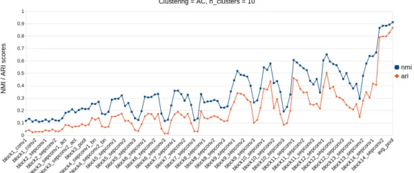
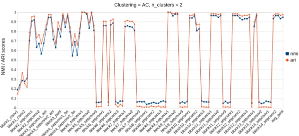
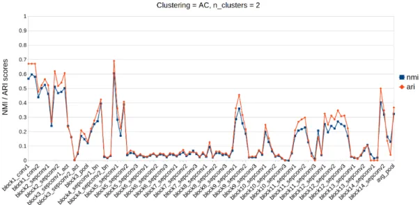
This thesis compares the results of clustering image sets by features extracted using different layers of a convolutional neural network. The image features were extracted with layers of a pre-trained image clas-sification network which layer weights were trained with ImageNet dataset. Eight image sets were used to test which extracted features achieve the best clustering accuracies. Features from the test image sets were extracted with the layers of the network architecture, and the features were clustered on a layer by layer basis. The clustering accuracies were measured with normalized mutual information (NMI). The results show that the clustering accuracies depend on the char-acteristic of the image set being clustered. The image sets with more than two image categories had the best NMI scores with the features from the second last layer in the architecture, while the image sets with two categories had different layers give the best NMI scores. Moreover, the image set with blurred images had the best result come from few of the first layers, showing that the current method of selecting the second last layer for feature extraction in pre-trained CNNs is not always optimal.

Keywords: Feature extraction, transfer learning, dimension reduction, Xception, agglomerative clustering, UMAP

TIIVISTELMÄ

Tässä työssä vertaillaan kuvajoukkojen klusterointituloksia eri piir-teillä. Piirteiden irrotukseen kuvista käytettiin valmiiksi koulutetun konvoluutio neuroverkon eri tasoja. Neuroverkko oli koulutettu kuva-luokitteluun ImageNet datajoukolla. Kahdeksan kuvajoukkoa kluste-roitiin eri piirteillä, jotka oli irrotettu neuroverkon eri tasoilla. Näiden kuvajoukkojen klusterointitarkkuus mitattiin parhaan piirreirrotus ta-son löytämiseksi kullekin kuvajoukolle. Klusteroinnin tulos mitattiin normalisoidulla yhteisen informaation metriikalla (normalized mutual information).

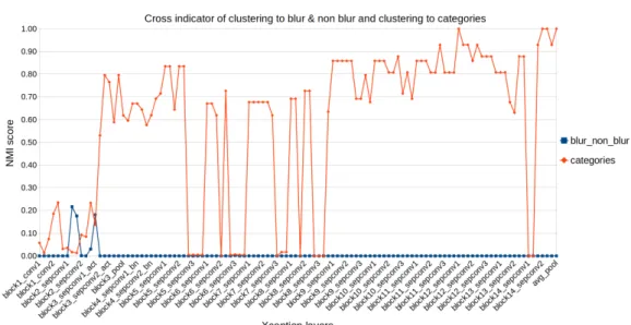
Työn tulos osoitti, että klusterointitulos taso tasolta mitatessa riip-puu klusteroitavasta kuvajoukosta. Kuvajoukot, jotka sisälsivät kuvia useammasta kuin kahdesta kategoriasta, klusteroituvat parhaiten ver-kon toiseksi viimeisellä tasolla irrotetuilla piirteillä. Kahden kategorian kuvajoukkojen parhaat klusterointi tulokset tulivat eri tasoilla. Kuva-joukko joka sisälsi kuvia sumeista ja tarkoista kuvista, saavutti par-haat klusterointitulokset piirteillä, jotka oli irrotettu verkon ylemmil-tä tasoilta. Tulokset osoittavat, etylemmil-tä yleisesti käytetty menetelmä valita valmiiksi koulutetun verkon toiseksi viimeinen taso piirreirrotukseen ei aina anna optimaalista tulosta.

Avainsanat: Piirreirrotus, siirto-oppiminen, dimensionaalisuuden pie-nentäminen, Xception, agglomeratiivinen klusterointi, UMAP

ABSTRACT TIIVISTELMÄ TABLE OF CONTENTS FOREWORD ABBREVIATIONS 1. INTRODUCTION 8 2. CLUSTER ANALYSIS 10 2.1. K-means . . . 10 2.2. Agglomerative Clustering . . . 11 2.3. DBSCAN . . . 12 2.4. HDBSCAN . . . 13

2.5. Clustering parameter selection . . . 18

2.6. Cluster validation . . . 18

2.6.1. Internal criteria . . . 18

2.6.2. External criteria . . . 19

2.6.3. Relative criteria . . . 20

2.6.4. Other validation methods . . . 20

3. CONVOLUTIONAL NEURAL NETWORKS 21 3.1. Structure . . . 21

3.1.1. Convolution layer . . . 22

3.1.2. Activation layer . . . 24

3.1.3. Pooling layer . . . 24

3.1.4. Other elements of advanced CNNs . . . 25

3.1.5. Hyperparameters . . . 26

3.2. Training . . . 27

3.2.1. Transfer learning. . . 28

3.2.2. Available datasets for CNN training . . . 28

3.3. Xception . . . 28

4. FEATURE DIMENSION REDUCTION 31 4.1. PCA . . . 31 4.2. UMAP . . . 32 5. DATASETS 34 5.1. ImageNet10 . . . 34 5.2. flower&qr. . . 34 5.3. Tools. . . 35 5.4. overcast&lowlight . . . 35 5.5. cab&chicken. . . 35

6. IMPLEMENTATION AND RESULTS 37 6.1. Experimental Setup. . . 37 6.1.1. Pipeline. . . 37 6.1.2. Hardware limitations . . . 39 6.2. Quantitative results. . . 39 6.3. Qualitative results . . . 47 4

The advent of deep convolutional neural networks has sparked our curiosity for advancing machine learning. As new network architectures are developed at an ever-increasing speed, this thesis was done to inspect what capabilities lie inside of these networks and how these capabilities can be used in the domain of unsuper-vised learning. I had the privilege to research several machine learning topics for this thesis and deepen my knowledge of machine learning methodologies, which will have a great influence on my upcoming endeavours as a machine learning professional. This thesis would not have been possible without the support of Visidon Oy. I would like to thank the whole staff of Visidon for providing inspir-ation, ideas and great 8-pool matches with me during my thesis work. Special thanks to my technical supervisor Sami Varjo and principal supervisor Miguel Bordallo Lopez for their valuable feedback.

Oulu, 4th October, 2019

ANN Artificial neural network

ARI Adjusted Rand index

CNN Convolutional neural network

DBSCAN Density-Based Spatial Clustering of Applications with Noise

HDBSCAN Hierarchical DBSCAN

ILSVRC ImageNet Large Scale Visual Recognition Challenge

NMI Normalized Mutual information

PCA Principal component analysis

ReLU Rectified linear unit

SGD Stochastic gradient descent

UMAP Uniform Manifold Approximation and Projection

K number of clusters

ε minimum distance

minpts minimum number of points

d(xp, xq) pairwise distance

dcore core distance

dmreach mutual reachability distance Gmpts Mutual Reachability Graph

λ density level

ER Relative Excess of Mass S(Ci) cluster stability

The goal of image set clustering is to group similar images to the same groups and dissimilar images to different groups. Let us have an example of an im-age set clustering. There is probably hundreds if not thousands of photos in a smartphone. If I would ask to group all of the photos to subgroups, with similar images in the same group and dissimilar images in different groups, what kind of subgroups there would be? Maybe a group of photos including pets, or a group of selfies taken on vacation with family, or even a group of failed photos. The boundary of similar and dissimilar photos in groups is intrinsically related to the set of photos you have.

To measure the image similarity algorithmically, we need to find a measure from the images which can be used to compute the similarity of the images. For example, one could use similarity measurement between the pet photos and va-cation selfies. In the domain of computer vision, images are commonly reduced to features for classifying algorithms to be able to classify the complex concepts of images [1]. The state-of-the-art image featurization methods are a group of machine learning techniques called artificial neural networks (ANNs), and pre-cisely the subgroup of deep convolutional neural networks (CNNs). Convolutional neural networks are non-linear estimators that can be used, for example, to clas-sify images to categories by training the network to learn features from the images. The network is trained with example input-output pairs of images and their cor-responding category, e.g. a group of vacation selfies which are categorized as selfie and group of pet images which are categorized as pets.

CNNs consist of different layers of mathematical operations which are stacked on top of another, previous layers output being the input of the next layer. Each of these layers learns to extract particular features known as feature-maps. The nature of how CNNs are trained means we do not know exactly what features each layer learns to extract, but the principle is that first layers learn more general features, i.e. features found in many images, like patterns of simple shapes, while deeper layers learn more complex features i.e. features which are more specific to the images in the training image set [2].

Now in this thesis, we were interested in using the different features which can be extracted with pre-trained CNN layers, as the clustering similarity meas-urements to test how different image sets can be clustered with these features. Relative works similar to this thesis are [2, 3], where [2] shows how the features change from general features to more specific features when deeper layers of pre-trained CNN are used to extract the image features. They also discussed on the transferability of the features to other tasks i.e. using the pre-trained CNN for classification on other image sets. In [3], the researchers showed how image features extracted with pre-trained CNN can be used to cluster images to cat-egories. They also briefly mentioned how selecting different layers to extract the features affect the clustering accuracy. This thesis studies more closely how the selection of different layers as feature extractors affect the clustering accuracies of the image sets by testing multiple layers as feature extractors.

The benefits for testing the feature extraction capabilities of pre-trained net-work is in the resources needed to train new netnet-works from scratch [4, 5]. If the

be clustered to correct groups, the layer had extracted features from the images which distinguish the images from another, and thus these features could be used as a similarity measurement between the images in the selected image set. As noted in [2], deeper layers learn to extract features more specific to the training set of the CNN, and upper layers learn to extract more general features. Thus testing all of the layers of one CNN architecture was conducted to find out which kind of similarities could be measured from the extracted features.

The scope of this thesis is limited to one CNN architecture, the Xception ar-chitecture developed in Google [6], with pre-trained weights for image classifying, trained with ImageNet dataset. Following the results of [3], which shows that im-age set clustering paired with Xception as feature extractor gives the best results in image clustering tasks.

The implementation part of the thesis compares how the features extracted with each layer are clustered. The cluster accuracies are measured by using labelled image sets and external validation metrics. The features are extracted from multiple image sets, and clustering accuracies are measured for each. The selection of the clustering algorithm and dimension reduction method for the clustering is also considered.

This thesis contains first the introduction to cluster analysis and examples of the used clustering algorithms. This is followed by an introduction to convolu-tional neural networks and the used Xception architecture. Dimension reduction of the features for clustering is briefly discussed in chapter four. The used datasets are presented in chapter five. The implementation and results are displayed in chapter six. Lastly, the discussion of the results is held in chapter seven, followed by conclusions in chapter eight.

2. CLUSTER ANALYSIS

Backer and Jain define cluster analysis as “In cluster analysis, a group of objects is split up into a number of more or less homogeneous subgroups on the basis of an often subjectively chosen measure of similarity, such that the similarity between objects within a subgroup is larger than the similarity between objects belonging to different subgroups.”[7], while Hansen and Jaumard write “Given a set of entities, Cluster Analysis aims at finding subsets, called clusters, which are homogeneous and/or well separated.”[8]. These definitions give the basis of clustering, which is to find a subset of a given set in which each subset contains similar objects and other subsets having dissimilar objects. The similarity measurement of images in the image set could be the shape of an object in the image, or the colour of the object, or some other measurable quantity from the image. In this thesis, the set of entities or group of objects which are being clustered are the features ex-tracted from the images. The clustering algorithm’s objective is to find separable subgroups of these features.

The clustering techniques explained in this chapter are categorized as parti-tional clustering, hierarchical clustering, and density-based clustering algorithms, based on the properties of the generated clusters. Partitional clustering al-gorithms directly partition the group of objects to a predefined number of clusters, without defining any hierarchy for the clusters [9 p.63]. Hierarchical clustering algorithms construct a hierarchy of clusters by partitioning the data sequentially, generating hierarchy from where all of the data points are in one cluster to each data point being a single cluster or vice versa [9 p.31]. Density-based clustering algorithms cluster data points by representing the data points by their density conditions (distance and number of nearest neighbours) on the clustering space [10]. Density-based clustering algorithms are tolerant to noise, as low-density points can be disregarded from the clustering as outliers or noise [11].

This chapter introduces the most common clustering methods, including the methods used in the implementation part of this thesis, the agglomerative clus-tering and the current state-of-the-art HDBSCAN. There is also a brief discussion of how the clustering parameters are selected for the implementation part, and the chapter finishes on summarising different validation metrics for clustering.

2.1. K-means

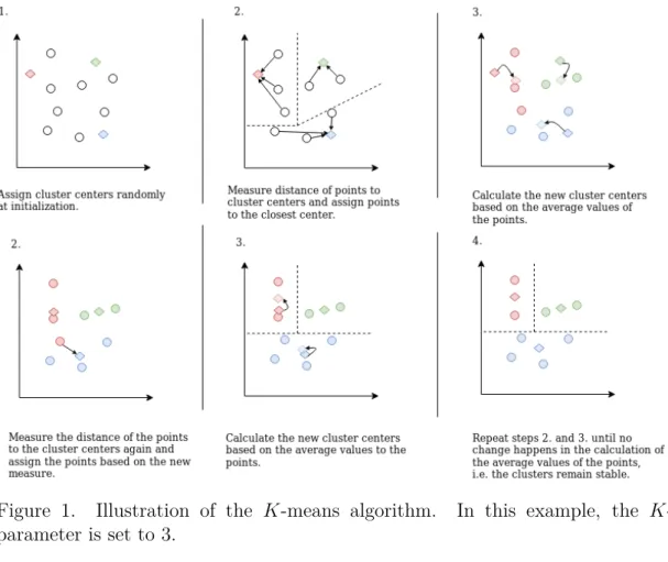
K-means clustering is a partitional clustering algorithm [9 p.68]. K-means par-titions the dataset to K groups in an iterative process. In native K-means im-plementation, the number of wanted clusters is given to the algorithm as the

K parameter. The algorithm is initialized by assigning a K number of cluster centres (centroids) at random on the dataset space, initially partitioning the data-space to K partitions. The partitioning is updated in alternating between two steps. The two steps consist of assigning the data points to the nearest centroid, by calculating the Euclidean distances of the data points to the centroids, and updating the centroid locations based on the calculated mean values of the data points assigned to the centroid. The algorithm finishes when no changes appear

to the clusters, e.g. the clusters remain stable. [9 p.68]. The K-means algorithm steps are illustrated in Figure 1.

The advantage of K-means is that it is a fast and quite simple algorithm to implement. It also clusters all the data points, i.e. it does not have a noise group. This can also be seen as a limitation of the K-means because it needs to expand the clusters to outliers which can alter other quite densely packed groups. Other limitations of theK-means are the random initialization of the algorithm, which means the partition changes between runs, and that the K parameter needs to be given before the clustering, i.e. the optimal number of clusters is left to be determined by the researcher.

Figure 1. Illustration of the K-means algorithm. In this example, the K -parameter is set to 3.

2.2. Agglomerative Clustering

Agglomerative Clustering or (AC) is a hierarchical clustering method. In AC each data point being clustered is first considered being on their own cluster [9 p.32]. These clusters are merged by their proximity (distance function) to another cluster. This merging is continued until all the points are assigned to one cluster, or when there is a wanted number of clusters.

The parameters for the AC are the distance function and the number of wanted clusters. The distance function is used to measure the proximity of the clusters to be merged, which is also called the linkage of the clusters [9 p.33]. One

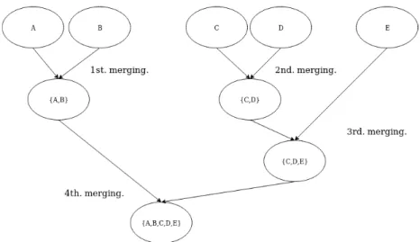
link-age method is Ward’s method, which minimizes the change in variance between clusters, and merges the clusters with the minimum value of this criterion [12]. AC generates hierarchy for the merged clusters and the wanted number of clusters is selected by cutting the hierarchy on the level which results for the wanted num-ber of clusters. Agglomerative clustering can be visualized as a tree structure, where single clusters are leaf nodes and merged clusters branch downwards the root, this is illustrated in Figure 2.

Figure 2. Agglomerative clustering visualization as tree structure. (A), (B), (C), (D) and (E) points are first their own clusters. The closest clusters of each other by the selected distance metric are the clusters (A) and (B), which are merged to cluster {A, B}. In the second step the distance of clusters is measured between clusters {A, B}, (C), (D) and (E), the clusters closest to each other in the second step are the clusters (C) and (D). This measuring of closeness and merging is continued and in the third step the closest clusters are the cluster {C, D} and (E) and in the fourth step the clusters {A, B} and {C, D, E} are merged.

2.3. DBSCAN

Density-based spatial clustering of applications with noise (DBSCAN) is a density-based clustering algorithm developed by Ester et al. [13]. DBSCAN operates by grouping data points which are packed densely together to clusters and points which are far away from other points (low-density regions) to noise. The points which are being clustered can have three properties in the DBSCAN point of view, the point can be a core point, a reachable point, or an outlier (noise). The parameters needed for DBSCAN are the minimum distance or ra-dius (marked as epsilon ε) and minimum points (minpts) parameters. ε is the metric from which distance away from the other points, a point is determined to be reachable. The minpts parameter sets how many points need to be reach-able of the point (the point itself included) to be converted as a core point. The core points form clusters with the reachable points that are within the given ε

distance from the core point. Outliers are points which are non-reachable to the core points. [9 p.221]

Clusters are formed with all the points reachable by the core point (including, other core points). New clusters are formed when core points are not reachable from each other. Different steps of the algorithm are illustrated in Figure 3.

The advantage of DBSCAN is the ability to generate clusters with arbitrary shapes and good scalability [9 p.220]. Some of the limitations of the DBSCAN is the choice of suitable parameters [14]. The minpts parameter can effectively restrict the forming of clusters. If the minimum points needed to form core points is set too great, natural clusters with fewer data points might be clustered as noise. The selection of the distance parameter ε can be problematic for high-density datasets. Selecting too high ε will cause all the data points to become reachable and then be clustered to one cluster. Selecting too small ε in already densely packed points might cause a division into multiple clusters. As the parameters are the same for the whole dataset being clustered, DBSCAN can only provide clusters based on a global density threshold [14].

Figure 3. Steps of DBSCAN algorithm. The minimum distance is set to epsilon

ε and the minimum points is set to 3. The first column shows the points. In the second column, the distance ε is drawn for all the points. The last column shows the assigning of the points to the core, reachable and noise points. The red points are core points because the red points are within εdistance from the given

minpts (3 points, with the point itself included). The yellow point is reachable point because it is within ε distance of core point (red). The blue point is an outlier (noise) because it is not within the distance ε from the core point. The left side red points plus the yellow point are one cluster, while the red points in the right side are considered a second cluster and the blue point is clustered to noise group.

2.4. HDBSCAN

Hierarchical density-based spatial clustering of applications with noise (HDB-SCAN) is a density-based clustering algorithm, based on hierarchical density estimates. HDBSCAN was derived from DBSCAN by Campello et al. [14] and extends DBSCAN to a form of hierarchical clustering algorithm. HDBSCAN performs DBSCAN over differing epsilon (ε) values and tests the result to find a clustering that grants the best stability over epsilon [15].

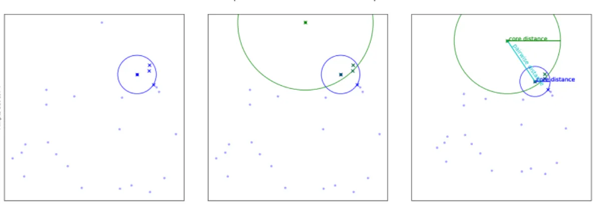
HDBSCAN removes the need for giving the minimum distance parameter epsi-lonεin DBSCAN, by running the DBSCAN only with minimum points (minpts) parameter. This indicates that every point (xp ∈ X) of the dataset will find

the minpts number of nearest neighbour points with differing pairwise distances (d(xp, xq)). The distance or radius which encloses the minpts number of points

is defined as core distance (dcore). Figure 4 illustrates the core and pairwise

distances with given minpts parameter. The core distance is needed for calcu-lating the mutual reachability distance (dmreach). Mutual reachability distance is

calculated with Equation (1) [14]

dmreach(xp, xq) = max{dcore(xp), dcore(xq), d(xp, xq)} (1)

The mutual reachability distance transformation is used to generate a weighted graph, which in the original paper is called the Mutual Reachability Graph (Gmpts)

[14]. The points of the dataset (x∈X) are the graph vertices and the dmreach is

the weight of the edges between the points it was calculated. From this graph, a

Figure 4. The points and their core distances with minpts value set to 4. The pairwise distance is calculated between the points. Mutual reachability distance is calculated between points by the Equation (1), which dictates that the dmreach

should always be the higher value between the core distances and pairwise dis-tance.

minimum spanning tree (MST) is extracted via the MST finding algorithm1_{. The}

resulting MST is shown in figure 5. The MST can be converted to a hierarchy of connected components by sorting the MST edges by their distance and iterating through the edges, and then merging the edges with the closest edge to new groups [15].

The result of the merging of the edges can be viewed as a dendrogram (a dia-gram representing a tree structure), which is shown in figure 6. From this dendro-gram, we could get clusters similar to in DBSCAN by drawing a horizontal line through the dendrogram by the distance value of the parameter epsilon. How-ever, in HDBSCAN this is done automatically by condensing the dendrogram to

1_{Graph theory and the related minimum spanning tree algorithm are out of scope of this} thesis, one used minimum spanning tree algorithm is Prim-Djikstra algorithm which is defined in paper [16].

Figure 5. Minimum spanning tree generated from the Gmpts. Figures 5-8

gener-ated via HDBSCAN software package [15]

Figure 6. Connected components dendrogram, generated from the minimum spanning tree of the graph Gmpts.

a less branched dendrogram based on the stability of the clusters. The condensed dendrogram is shown in figure 7. The stability of the cluster Ci at level λ in the

dendrogram is calculated with the concept of Relative Excess of Mass (ER) of a

cluster Ci. The ER at level λmin(Ci) is calculated by Equation (2) [14] ER(Ci) =

ˆ

xCi

(λmax(x, Ci)−λmin(Ci))dx (2)

where theλmax(x, Ci) is the density level where Ci is split or it disappears. The

discrete case of Equation (2) for finite dataset size X is formulated as Equation (3) [14], S(Ci) = X xjCi (λmax(xj, Ci)−λmin(Ci)) = X xjCi ( 1 εmin(xj, Ci) − 1 εmax(Ci) ) (3)

where λmin(Ci) is the minimum density level at which Ci is defined as cluster.

The parameter λmax(xj, Ci) is the maximum density level where the object xj

belongs to cluster Ci, and εmax(Ci) and εmin(xj, Ci) shows the correlation of λ

level to corresponding ε values [14]. Now the clusters can be selected from the condensed dendrogram (figure 8). The resulting selection shows that two clusters were found in the data and the data points outside of the selected λ values are grouped as noise. The clustered dataset is shown in figure 9, where the dark points belong to the noise group and the yellow and green points are the points that are assigned to the clusters.

Figure 7. Condensed dendrogram, by the stability of the clusters.

HDBSCAN’s advantage over DBSCAN is that it is not limited to one density threshold. HDBSCAN can calculate DBSCAN like densities with an infinite range of density thresholds and construct a simplified tree structure from the most significant clusters. From this tree structure, the optimal threshold can be selected based on the stability of the clusters [14], effectively removing the problem of selecting optimalε in DBSCAN. Even the added steps in HDBSCAN does not make it slower than DBSCAN [17] and such is a generally a better alternative to use over DBSCAN.

Figure 8. Select the clusters based on the stability S(Ci).

2.5. Clustering parameter selection

Many of the discussed clustering algorithms have parameters that need to be assigned before clustering. The main parameters for the algorithms used in the implementation are the number of wanted clusters in the case of AC and the minimum points in HDBSCAN. The other parameters are the distance metric to calculate the distances between the points in HDBSCAN, and the linkage method in AC. These parameters affected the clustering outcome, and usually, they are selected based on the dataset being clustered. However, this needs to be done automatically or left for default values if the dataset is unknown.

In this thesis, the number of wanted clusters for the AC algorithm is selected based on the dataset being clustered. The number of groups in the datasets are known as the images in the datasets have labels on them. The linkage method for AC is selected to be Ward’s method.

The distance metric parameter is set to Euclidean, which is the default dis-tance metric in the implementation of HDBSCAN. In HDBSCAN the number of minimum points is left for the default value of 5. This default minimum points value is not optimal for each of the datasets, but as leaving the value as default, we eliminate the parameter tuning for this clustering algorithm and only focus on how the under-laying features affect the clustering outcome.

2.6. Cluster validation

Validation of the clusters is derived based on a selected metric once the data set is clustered. The clustering validation metrics can be classified into three groups, which are internal criteria, external criteria and relative criteria [9, 10]. The internal validation criteria are used for unknown data sets without labels, and such, the validation of the clusters could be the clustering object itself. External validation criteria can be used in data sets with known structures, like image-sets with image labels. Relative validation compares two clusterings of the dataset, either with the same algorithm with different parameters or clusterings with dif-ferent clustering algorithms. The next sections explain the validation criteria more in-depth and introduce the selected algorithms that are used for validating the cluster outcomes in this thesis.

2.6.1. Internal criteria

Internal criteria are used to measure the validity of the generated cluster struc-ture without prior (external) information about the clusters. The internal validity comes from the objective of the clustering, which was generating groups where similar objects are in the same group and distinctive objects in different groups [18]. The basic measurements for validating unknown data sets are the compact-ness and separation of the data points in the generated clusters. The internal validation methods do not give insight about if the clusters are correct or

mean-ingful on the application domain, but the internal validation measurements can be used to calculate the optimal number of clusters for the given data set [18].

One algorithm used in measuring the quality of the cluster structure is the silhouette technique [19]. The silhouette value is calculated for one data point at a time, based on the distances to other clustered data points. The silhouette value scales in a range from -1 to 1, 1 meaning the data point is appropriately clustered and -1 means the data point would naturally belong to the neighbouring cluster, i.e. the cluster it belongs is “wrong” based on the distance calculated. The silhouette value for point i is calculated at the following Equation (4) from [19]:

s(i) = b(i)−a(i)

max{a(i), b(i)} (4)

where a(i) is the average dissimilarity of point i to all other objects in the cluster it is assigned, marked as A. d(i, C) is the average dissimilarity of ito all objects in the other clusters C. b(i) is calculated as b(i) = minC6=A(d(i, C)) for

all the clusters C, except for the cluster the i belongs (A). From Equation (4), we can formulate the range as −1≤s(i)≤1 [19].

2.6.2. External criteria

External criteria assume having information about the data structure before clus-tering the data. After clusclus-tering the data, we compare this prior information to the generated structure of the clustering [10]. In image-set clustering, this prior structure of the dataset means we have prior knowledge about which images be-long to the same group and which don’t, e.g. the labels of the images. Two example indexes for measuring the external validation are the Adjusted Rand Index (ARI) and Normalized Mutual Information (NMI). The Rand index is a measure of similarity between two clusterings [20] and the Adjusted Rand Index, is adjusted for the chance of grouping elements to correct groups, i.e. ARI out-puts similarity values for groups with more similarity than randomly assigning elements to clusters.

The ARI is calculated using the Equation (5), where U and V are different clustering of the same dataset, e.g. the U could be the clustering results of running the clustering algorithm, and the V could be the clustering based on the given labels for the images.

ARI(U, V) = 2(N00N11−N01N10)

(N00+N01)(N01+N11) + (N00+N10)(N10+N11) (5)

The indexes, N00, N01, N10 and N11 are defined as follows: N11 is the number of data point pairs that are in the same cluster in both U and V clusterings. N00

is the measurement of pairs in different clusters in both U and V, while N01 is

the number of pairs which belong to the same cluster in U but are in different clusters in V. N10 is the number of pairs which belong to the same cluster in V

but are in different clusters inU. [21] ARI scores near 0.0 means random labelling and ARI score of 1.0 means perfect match [22].

The NMI is information theoretic based measure and NMI is defined via mar-ginal and joint distributions of data in the clusterings U and V. The mutual information (MI) is expressed as I(U, V) which is defined as H(U)−H(U|V) =

I(U, V). H(U) and H(U|V) are calculated as in [21]

H(U) = − R X i=1 ai Nlog ai N, H(U|V) = − R X i=1 C X j=1 nij N log nij/N bj/N

The MI can be normalized with multitude of generalized mean methods likejoint,

max, sum and sqrt, just to name a few [21]. In this thesis, the MI is normalized with the sqrt method and the NMI is calculated as in Equation (6) [22]:

N M I(U, V) = I(U, V)

mean(H(U), H(V)) (6)

External criteria give a valid measurement of the clustering quality, but as it relies on the class labels, it is not a suitable measurement for datasets without labels or unknown data.

2.6.3. Relative criteria

Relative criteria can be seen as a measure of the utility of the clustering algorithm. Relative validation criteria can be the selection of clustering parameters or clus-tering algorithms, which best fit the dataset being clustered [10]. In this thesis, the relative validation criterion is to use two clustering algorithms for the se-lected datasets. In the labelled datasets, both clustering algorithms use NMI for external validation, and the resulting NMI values are used to evaluate if the change in the NMI values were due to differences in clustering algorithms or the differences from the datasets.

2.6.4. Other validation methods

Manual inspection can be used as a validation method when the objects being clustered can be inspected, like images. The manual inspection of clusters can be used to verify unlabelled datasets, where the usage of the external validation measures are not possible. Manual validation is usually conducted by a domain expert.

3. CONVOLUTIONAL NEURAL NETWORKS

Convolutional neural networks (CNNs) are non-linear function estimators, which work by the principle of learning a function f which maps the given inputs x to some defined outputs y,

f(x) = y (7)

by learning the function with example input-output pairs. In the case of im-age classification CNNs the network is trained on with input imim-ages and their corresponding classes. After training the CNN, it is used to predict on which class the feed input image belongs. The main difference of convolutional neural networks over other artificial neural networks is that they have least one or more convolution layers, which can be used to process data that has grid-like topology, like image data, which can be seen as a 2-D grid of pixels [23 p.326].

CNN derives its idea from biological visual systems where studies of the mam-mal visual system [24] determined that the first parts of the visual system respond to patterns of light coming from simple shapes to the receptive fields. This idea is carried over to CNNs as the convolution operation on the first layers of the architecture tries to mimic this biological process by activating on similar shapes of the input image as detected by the biological receptive field of cells. The first implementations derived from this idea date back to 1980 when Fukushima presented the Neocognitron [25].

One of the first modern CNN for visual recognition was the network LeNet-5 which was trained using backpropagation and was used for handwritten digit recognition [26]. More recent CNNs use similar stacked-layer architectures which use tens to hundreds of layers, while their predecessor LeNet-5 contained only seven layers. Modern architectures use a multitude of different techniques to increase the accuracy of the networks and ease their training. On the next section, the basic structure of a CNN and the elements within are explained.

3.1. Structure

The CNN structure depends mostly on the selected architecture, but they all share similar basic building blocks. The building blocks of any CNN are the layers of the CNN. Usually, the layers of CNNs consist of operations like convolu-tion, activaconvolu-tion, and pooling. These operations are illustrated in figure 10. The convolution operation is the dot product of the input and the layer’s kernel (or filter). This produces a set of linear activations. The activation function is used to scale the linear convolution outputs to non-linear activation maps. Pooling operation modifies the input by taking, for example, average or maximum values of certain sized rectangle neighbourhood of the input and passing these values to the next layer effectively downsampling the input.

Figure 10. The basic operations of convolutional neural network.

A dense layer with softmax activations is operation found in the last layer of the network. The dense (or fully connected) layer with softmax activation functions is used to map the inputs to the predicted class. Softmax function works by distributing the input values to the layer as predictions from 0 to 1 to the classes, and the highest prediction being the class the network has classified the input image. Figure 11 shows an example of image classification done with CNN.

Figure 11. Image classification example with Xception CNN architecture. The CNN takes RGB images sized 299 by 299 pixels as input. The first convolu-tion layer has 32 filters for each channel (RGB) and each filter consist of 3×3 size kernel, with trained weights. The output of the first convolution layer is the convolution between the filter weights and the input images channels, each channel result summed as feature map with 32 features size 149 by 149. The previous layers feature map is feed to the next layer, which results for another feature map. In the average pooling layer, the feature map is reduced to a vector of size 1×2048, which is feed to a dense layer, which reduces the features to a vector of size 1×1000. From this feature vector, prediction of the image class is concluded by taking the softmax of the vector and mapping the highest value to the corresponding class.

3.1.1. Convolution layer

The heart of the CNNs is the convolutional layer. The convolutional layers consist of a group of kernels which have learnable weights (or parameters). The convo-lution operation is a dot product over vectors, which is presented in Equation (8) (from [23 p.328, Fig.9.4]). The equation is a discrete case of the convolution shown for two-dimensional image (I) and kernel (K).

S(i, j) = (I∗K)(i, j) =X

m

X

n

I(m, n)K(i−m, j −n) (8)

When the convolution is expanded to colour images, each colour channel is convolved separately by the corresponding kernel, which means that three channel colour image needs three separate kernels or a 3-dimensional filter. An example of a 3-dimensional convolution operation is illustrated in Figure 12. The dimensions of the feature map (output of the convolution) in the example are 2×2×1 because the convolution is summed over all the channels, e.g. the selected 3×3×3 filter has 27 values and the dot product is taken by these values and the corresponding area of size 3×3×3 of the image. As the image is larger in x and y dimensions, the

filter is slided over the image, such that the whole image is convolved sequentially.

Figure 12. Example of a 3-dimensional convolution for three channel colour image. While the kernel size may vary depending on the implementation, the kernel size is usually smaller than the input size. When the kernel size is smaller than the input the convolution is said to have sparse interactions or sparse weights. This property is important to CNNs because images can have thousands or mil-lions of pixels, but even small-sized chunks of the image can be used to extract important features of the image like edges. With this property, the filters can extract meaningful features from the image, with fewer parameters than having to save the parameters for every pixel. [23 p.330]

The input image’s size reduction can be controlled by zero-padding the input image’s edges with a layer of zeros. For the example in figure 12, zero-padding the image would result in the image’s size to be raised to 5 ×5 ×3 and the

convolution with the same kernel size of 3×3×3 would result in output of size 3×3×1. The reduction of input image’s size can be calculated with Equation

(9) where O is the output size of heighth and widthw, while I is the image size and f is the kernel size.

O(h, w) = (Ih−fh+ 1),(Iw−fw+ 1) (9)

The result of the convolution (feature map) is feed to the next operations of the architecture. The convolution operation works the same for feature maps. The

parameters of the convolution layer, are the weights of the kernel, the dimension of the kernel and stride which are explained in section 3.1.5.

3.1.2. Activation layer

Activation layer’s primary function is to add non-linearity to the network. Non-linearity is needed to approximate linear problems. There is different non-linear activation functions which can be used like sigmoid, tanh, ReLU and their variants. ReLu is probably the most commonly used activation function in CNNs. ReLU maps the output values of the convolution to values from zero to upwards via transfer function as shown in Equation (10) [27].

f(x) = max(0, x) (10)

This way the negative values are removed from the convolution output and positive values have linear mapping, making the ReLU non-linear with the trans-formation. The activation transformation results in an output which is referred to as the activation map.

3.1.3. Pooling layer

Pooling layers act as statistical summaries of the feed input by calculating a single value from the neighbouring values of the input. The benefits of pooling are to make the input spatially invariant to small translations, which correlates for better generalisability of the features, and downsampling the input, making the following computations more efficient. For example in the case of max-pooling, the max value of the selected input area is passed to the next layer. If this max value’s position changes a little, but within the area of the pooling operation the same max value is selected, and the pooling layers output stays the same [23 p.335-338]. However, the downsampling in max-pooling causes aliasing1 which can decrease the accuracy of the network [29]. The suggested solution for the aliasing problem is to add anti-aliasing filter to the pooling operation.

The pooling layer parameters are the pooling operation, the size of the pooling operation, and the stride. Two common pooling operations are max-pooling, which selects the maximum value in the pooling area, and average pooling, which averages the values of the pooling area and passes this value forwards. Max-pooling is illustrated in Figure 13.

1_{Aliasing is a phenomenon related to the sampling theorem. Aliasing occurs when the} sampling of signal (discrete in digital) is below the Nyquist frequency. More of the sampling theorem, effects of aliasing and how to mitigate them with anti-aliasing can be found in the book ’Practical Digital Signal Processing’ by Edmund Lai [28 p.15]

Figure 13. Max-pooling with pooling area size 2×2 pixels and stride 2. Figure

from [30].

3.1.4. Other elements of advanced CNNs

As the available computing power increases, more complex architectures have been developed. Usually, the simplest way to achieve improved classification accuracies is to increase the labelled training data, but as the training data in-creases, so does the training time. Better architecture designs are constantly needed. Some additions to the typical set of layers and techniques are residual learning [31], batch normalization [32], inception module [33] and depthwise sep-arable convolutions [34], which further increased the accuracy and trainability of the networks.

Residual learning adds skip connections to the network, where layer outputs are added to inputs of layers deeper in the architecture, as well as passing the output to the next layer [31]. The network has fewer layers to learn in the early stages of training, because of the skip connections, and thus easing the problem of vanishing gradients (for vanishing gradient, see section 3.2). A residual block is illustrated in figure 14.

Figure 14. Residual learning, figure modified from [31].

Networks that use batch normalization can be trained with higher learning rate (for learning rate, see section 3.2), which theoretically accelerates the training of the network. Ioffe and Szegedy argue that the batch normalization works by reducing the internal covariate shift [32], but some experimental studies [35] show that this might not be the cause. The exact mechanism of how the batch normalization works is still discussed, but the benefits of using it are evident [36].

A Inception module adds multiple convolutions with different kernel sizes to one layer, making it wider. The idea behind making the network wider is that the kernel size limits how small or big features the kernel can search from the image. When adding three convolution kernels with varying size (1×1, 3×3

and 5×5 in the paper) the convolution operations can look for differently sized

features, making the architecture more accurate. More convolutions make the network more computationally demanding, and thus the inception module has

1×1 convolutions before the different sized kernels, to limit the input channels

sizes, making the convolutions less computationally demanding [33]. A Inception module is shown in figure 15.

Finally, depthwise separable convolution performs first channel-wise (depth di-mension) spatial convolution and is then followed by 1×1 convolution [6].

Figure 15. Inception block, figure modified from [33].

3.1.5. Hyperparameters

The layer parameters can be divided into fixed and learnable parameters based on if the parameters change when CNN is being trained. The fixed parameters are the kernel size and stride. The learnable parameters are the weights of the convolution layer’s kernel. The kernel size and the weights determine what the operation returns. A convolution kernel has three parameters which are the size of the kernel, the stride and the weights. Pooling layers have only fixed parameters which are the size and the stride. The kernel size determines how many neighbouring values affect the operation, e.g. with kernel size 3×3 eight

neighbouring pixels (nine in total) affect the outcome value, being it convolution in convolution layers or pooling operation in the pooling layers. Stride is used to adjust the overlap of the operations by determining how many pixels the kernel moves while sliding over the input, in cases where the kernel size is smaller than the input.

The weights are the most important part of the convolution kernel because it determines which kind of shapes are looked in the kernel sized area of the

input. As the weights are randomly initialized at first, they look for arbitrary shapes, but as the weights are adjusted in the learning part, the kernels learn to look for meaningful shapes from the input. The stride can be used on both convolution and pooling layers for downsampling the input size. Activation layers only parameter is the activation function.

3.2. Training

The objective of training the CNN is to change the convolution layer’s weights and other learnable parameters so that the CNN can output the wanted results, i.e. the prediction of the correct class of the given input. The weights, which are commonly initialized randomly at first, are the parameters the network learns by optimizing the error of the network. The error of the network is the difference of the prediction (class) and the correct class that the input belongs. As such, the network needs vast amounts of correct input-output pairs, e.g. image and its correct label, for training these weights when starting from a random state.

The basic building blocks for optimizing the error of neural networks are the optimization function, its parameters, and the backpropagation method. The backpropagation is a method used to calculate all the gradients (the change of the weights) from the output of the network to back to the input, using the dif-ferential chain rule [23 p.200-201]. The most used optimization algorithms are stochastic gradient descent (SGD) and its variants like SGD with momentum, RMSprop, AdaGrad and Adam [23 p.290-305]. The SGD updates the gradient values calculated by the backpropagation, by minimizing the error of the classi-fication by comparing the output of the network (category class) to the real class given to the network. One important parameter for the SGD is the learning rate, which is used to give boundaries for how much the optimizer changes the weights per run, which affects how fast the CNN learns. Too small learning rate and the error decreases very slowly, and too high learning rate and the error might not decrease at all.

Some of the problems which can appear in training are the overfitting and van-ishing gradient problems. Overfitting means that the weights learn the training-set too accurately, and the network loses its generalisability when presented with new unseen inputs to predict. Overfitting is usually the result of too small or poorly selected training-set or an architecture that has too much capacity (learn-able parameters) for the task complexity it tries to solve. Vanishing gradient is a problem which causes trainability issues for the upper layers of a deep network. The vanishing gradient occurs when deep networks usesigmoid ortanhactivation functions. The sigmoid and tanh activation functions map the activation values to a range of 0 to 1. Therefore, convolution outputs are ’squeezed’ to the narrow range of 0 to 1. After stacking multiple of these activation layers in the architec-ture, the high output values in the upper layers have a minuscule influence on the network’s output. When the layers influence for the output is minuscule, so is the error caused by the layers. The error of the upper layers diminishes to zero, and the gradients can not be calculated, which means the weights of the layers are not changed. Vanishing gradients can be avoided by using activation functions

that map the values on border range than the sigmoid or tanh functions. One such activation function is the ReLu.

3.2.1. Transfer learning

Transfer learning can be seen as a technique to take existing networks with learned weights on some domain (e.g. network trained with ImageNet) and use the net-work to some other relatively similar task, like extracting features from different image sets. The transferability of the weights is limited by the difference of the task the weights were trained on, and the task the weights are transferred. Usu-ally fine-tuning for the used domain is needed. Fine-tuning means training only the last layers of the network, which is usually much faster than training the whole network. It has been shown that pre-trained networks can learn general enough features to be used in transfer learning for other tasks [2, 37, 3]. The advantages of using a trained network for other tasks are the lesser amount of data and time needed to train the network. Training a network from the begin-ning needs a great deal of traibegin-ning data, which might not be available in some specialized cases, for example, medical imaging.

3.2.2. Available datasets for CNN training

There is an increasing number of publicly available labelled datasets, which can be used in image classification, object detection and recognition tasks, like Open Images [38], ImageNet [39], PASCAL VOC [40] and CIFAR [41] datasets. Prob-ably the most used dataset is the ImageNet and its subset, which is used in the ImageNet Large Scale Visual Recognition Challenge (ILSVRC). ImageNet dataset contains 14 million images from 21 thousand classes. ILSVRC subset contains 1.2 million categorized images with 1000 different classes from the Im-ageNet dataset [42]. ImIm-ageNet datasets contain images of objects ranging from everyday items to different species of animals. Because of the popularity of the ImageNet dataset, there is a lot of CNN architectures published with pre-trained weights which are trained with the ImageNet dataset. As is the case with the used Xception architecture, which has readily available framework (Keras) implement-ation with weights trained with the ImageNet dataset. CNN architecture, which was trained with ImageNet, was selected because of the availability of these ar-chitectures. These architectures have been shown to get comparable results with the ILSVRC dataset, which is a de-facto benchmark test for new CNNs.

3.3. Xception

Xception is a CNN architecture which novelty was the adaptation of modified depthwise separable convolution layers. Xception was developed in Google [6], and it is based on the previously published Inception [33] architectures, also de-veloped in Google. In Xception architecture, the Inception modules were changed

to the modified depthwise separable convolutions, and hence the name of ‘Ex-treme Inception’. Xception reached 0.790 Top-1 accuracy on ImageNet in 2016. Now (as of writing in 2019) the networks with similar parameter count achieve 0.826 Top-1 accuracy [43]. Xception was chosen to be the CNN architecture of study, because of its good performance on the ImageNet dataset, and the avail-ability of the pre-trained models with the ImageNet. Also, the readily available implementations of the architecture allowed for straightforward runs through dif-ferent layers of the architecture.

Xception architecture is illustrated in figure 16, where the separable convolu-tion layers are the modified depthwise separable convoluconvolu-tion layers. Xcepconvolu-tion architecture also includes the residual layers and batch normalization. Xception architecture can be seen to be split to 14 different blocks which are separated by the residual layers. The layers in the implementation also follow the 14 block separation in their naming, by grouping the layers by the corresponding block they belong.

Figure 16. Xception architecture, modified from [6]. The input images are first feed through the entry flow and then through the middle flow, which is repeated eight times, and finally through the exit flow. The logistic layer softmax produces the category predictions of the input image.

4. FEATURE DIMENSION REDUCTION

High dimensional data adds complexity for processing data [9 p.237]. The data complexity by high dimensions is usually referred as ‘curse of dimensionality’, a term coined by Bellman [44], which describes the exponentially increasing cost of algorithms with the growth in the number of variables (dimensions) [45]. Di-mension reduction (DR) is a technique used for alleviating the problems associ-ated with high dimensions. The basic principles of dimension reduction are the concatenation of most relevant features from the high number of available and insignificant features. This can be formalized as:

F(x) :Rd→Rd0

where DR is the mapping F which maps the high-dimensional feature space

Rd _{to a lower-dimension feature space R}d0 _{[9 p.238].}

Various clustering approaches are based on the assumption that there is a higher number of data points (N) in the dataset than feature variables (dimensions, d) in a single data point. Thus, dimension reduction can be useful in situations where the feature variables of a given data point are higher than the number of data points being clustered (N < d) [9 p.237]. The difference in clustering algorithms with high dimensional features can also be seen in experiments that compare the results of AC and HDBSCAN. Dimension reduction can also be used to visualize high dimensional features, by compressing the features to two or three dimensions. DR has limitations, as the process of which features to keep and which to discard is usually done via optimization of a cost function, which causes loss of information [9 p.238].

Dimension reduction algorithms can be categorized into linear and non-linear algorithms. Examples of linear algorithms are PCA [46] and ICA [47], while UMAP [48], LLE [49] and autoencoders [50] are examples of non-linear dimen-sion reduction algorithms. The algorithms selected to be used in this thesis are the linear principal component analysis (PCA) and the non-linear uniform manifold approximation and projection for dimension reduction (UMAP). PCA is probably the most commonly used linear dimension reduction method, while UMAP is a novel non-linear method (2018). UMAP is also great at visualizing high dimensional data [50] (also, see figure 17). The algorithms are introduced in more detail in the next sections.

Dimension reduction is usually used as a preprocessing step with high-dimensional feature spaces, which the output features of different layers are. For example, some of the layers can have output features with size 147×147×128, which

res-ults in features with over 2.7 million dimensions. However, as DR causes loss of information, the features in this thesis are also clustered without dimensionality reduction.

4.1. PCA

Principal Components Analysis (PCA) is a statistical method which can be used in data reduction, data compression and dimension reduction by finding a subset

of features which represent the majority of the data. PCA works by finding the single best subspace (Rd0) of the original feature space (Rd) within the criterion of least-square error [51]. This is achieved by searching orthogonal directions which maximise the variance of the dataset, assuming the feature-space is linear. Hence PCA can have problems with non-linear feature spaces. The search for orthogonal directions can be formalized as an error minimization functionJ which minimises the representation error E as follows (modified from [51])

JP CA =E    kx− d0 X i=1 (wi,x)wik2    (11) where orthonormal directions are vectors wi and x is a matrix of dataset

fea-tures in original d dimensions. Principal components (PCs) are derived from the orthonormal directions asP Ci,···,d0 = ((w_i,x), . . . ,(w_d0,x))t. The PCs with

max-imum variances are selected to represent the data points in the target dimension

d0 by selecting d0 number of PCs, in order that P C1 explains most of the

vari-ance of the dataset andP C2 the second-most, etc. [51]. If the wanted dimension

parameter is not specified, the PCs are generated for all the original dimension. This can be helpful when deciding to which dimensions the dataset is reduced, by looking how much variance each PC contains. For example, if the dataset being reduced contains features with 100 dimensions and the first two PCs contain 50% of all the variance and the other 98 PCs contain evenly spread out the last 50% of the variance, it could be useful to only use the first two PCs to represent the dataset in reduced dimension. However, the optimum number of PCs is highly application dependent.

4.2. UMAP

Uniform manifold approximation and projection for dimension reduction (UMAP) is a non-linear dimension reduction method, based on manifold learning. UMAP does dimension reduction by finding a low dimensional embedding of the data that approximates an underlying manifold [48]. The inner workings of UMAP in dimension reduction are based on theoretical frameworks of Riemannian geometry and topological algebra, which can be further inspected in the original paper [48]. The simplified principle of UMAP can be described in two steps, one where

k-neighbour based graph from the dataset is constructed and other where the low-dimensional layout of the graph is computed, which represents the dimension reduced version of the dataset. The strengths of UMAP for visualization come from the ability to pack similar points from the higher dimensions closer together in two dimensions, and the ability to keep enough global structure to have visu-alizations where there is enough separation between dissimilar points. This is illustrated in figure 17, which compares how the dimension reduction done with UMAP and PCA generates different plots. Both were used to reduce the same 2048 dimensional features to two dimensions.

UMAP implementation [52] has a multitude of hyperparameters, which can be used to fine-tune the algorithm. The parameters for the basic usage are the

Figure 17. UMAP and PCA mapping in two dimensions. 1000 features with a dimension of 2048 were reduced to two dimensions with UMAP and PCA, then clustered with AC. The colours represent the labels of for each cluster.

number of neighbours (k) used in the k-nearest neighbour search, the target dimensionality (d0) of the dataset, the minimum distance which controls how tightly the points are packed, and the metric to be used in the calculation of the pairwise distance matrix. Other parameters were left as default values, unless mentioned specifically.

One notion of UMAP regarding this thesis use case is the optimization of the low-dimensionality layout, which is based on the SGD optimizer. SGD uses sub-sampling for the optimization. This effectively means that the order of features feed to UMAP affects how the lower-dimensionality is constructed. As stated in the original paper ‘Since UMAP makes use of both stochastic approximate nearest neighbour search, and stochastic gradient descent with negative sampling for optimization, the resulting embedding is necessarily different from run to run, and under sub-sampling of the data.’ [48]. To get reproducible results when using UMAP as DR step before clustering, the features need to be feed in the same order for each run, and the sampling needs to have the same random seed number.

5. DATASETS

The clustering results and features extracted by the CNN highly depend on the images in the datasets. Eight image sets were selected to be used as evaluation datasets. The evaluation datasets are selected within the assumption that the datasets contain images with enough differences that the extracted features, by some of the layers, results in clusters forming. The requirements for the datasets depend on the selected validation metric. When external clustering validation is used, the dataset being clustered needs to have labels on the data. The dataset labels are compared to the labels given by the clustering algorithm. In this thesis, the selected clustering validation metrics were the external NMI and ARI scores, and thus the dataset being clustered needs to have labels.

The datasets were selected for testing the layers feature extraction capabilities based on different clustering tasks. The selected datasets and their clustering tasks can be seen in Table 1. Next subsections introduce the datasets more thoroughly.

Table 1. Properties of the evaluation datasets

Dataset Name Clustering Task Img. Size Classes Images

ImageNet10 Object detection Varying 10 500

flower&qr Object detection 256×256 2 500

Tools Object detection 640×480 7 560

overcast&lowlight Scene detection 256×256 2 500

cab&chicken, sigma2 Object / blur detection Varying 2 200

cab&chicken, sigma3 Object / blur detection Varying 2 200

cab&chicken, sigma5 Object / blur detection Varying 2 200

cab&chicken, sigma9 Object / blur detection Varying 2 200

5.1. ImageNet10

ImageNet10 is a dataset with images from 10 classes from the ILSVRC 2012 validation set, each class containing 50 images. As the used CNN was trained with ImageNet dataset, these classes selected from the validation image set represent the baseline dataset for extracting features which should generate good clustering results in the deeper layers. The selected categories from the ILSVRC 2012 validation set are jigsaw puzzle, dial telephone, ground beetle, analog clock, cup, hay, French bulldog, great grey owl, bearskin and steel drum.

5.2. flower&qr

The second dataset is the flower&qr dataset, that is constructed from in house datasets used for other projects. The flower&qr dataset was created by selecting images from two datasets, one category having images similar as in the CNN’s

training dataset, while the other category has images which are not explicitly used in the CNNs training set. The flower images should generate distinguish-able features with the CNN because the used training dataset (ImageNet) con-tains images of flowers. The second category in this dataset was selected to be compromised of images augmented with a QR-code image on top of the image because QR-code images are not explicitly trained with the CNN. As to test if the extracted QR-code image features can be separated from the flower images. The flower&qr dataset has two categories, each one having 250 images.

5.3. Tools

The dataset Tools was published by the authors of [3], which they used in their Xception feature extraction and clustering pipeline. The CNN architecture is the same as used in this thesis, and thus their dataset can be used as a validation method for the pipeline constructed in this thesis. The Tools dataset contains seven object categories with images of tools like allen key, clamp, driver, flat and images from pens, screws and USB sticks. The category images are constructed with five lighting and background conditions. All of the conditions and the objects are used as one mixed image set, having seven classes based on the object category, containing 560 images.

5.4. overcast&lowlight

The overcast&lowlight dataset contains images from two scene categories, a low light and overcast categories. The first category is constructed from low light images, e.g night time images where the major part of the image is dark while having some light sources in the image, of different things like objects and scenes, while the second category contains overcast (cloudy skies) images which are taken from objects and scenes in outdoor environments. The low light and overcast images can both have objects similar to the CNN’s training dataset, and thus the extracted features can be similar to images from both of the categories, as the dataset is labelled based on the scene of the images and not by the objects in the images. This dataset tests if the CNN’s features from some of its layers can be used to separate scene images. Theovercast&lowlight dataset has 500 images, 250 on both categories.

5.5. cab&chicken

The cab&chicken datasets are constructed from images in the cab and prairie chicken categories from the ILSVRC 2012 validation set. The datasets also con-tain blurred versions of the cab and prairie chicken images. The images were blurred with Gaussian blur, with a kernel size of 31×31 and with sigma values

2, 3, 5 and 9. The cab&chicken datasets are separated and named based on the value of the sigma used in the Gaussian kernel in the dataset. The cab&chicken

datasets have two clustering targets, cluster images to category groups or blurred and non-blurred image groups. These datasets are used to test if some of the features from the layers can be used to cluster images to groups based on blurri-ness. Additionally, these datasets are used to test how different amounts of blur in the images affect the clustering to the image categories. The datasets have 200 images, 50 for each group and 100 per class.

6. IMPLEMENTATION AND RESULTS

Within the increased usage of CNN based systems, there has been growth in readily available software packages and frameworks for developing and training CNNs. Few of the most used frameworks are TensorFlow, Torch, Keras, Theano and Caffe, which TensorFlow is probably the most popular. All of the men-tioned frameworks have application programming interfaces (APIs) or bindings to Python, which made the selection of the implementation programming lan-guage obvious. From the frameworks, TensorFlow was selected to be the baseline framework with supplementary high-level APIs from Keras. Additional librar-ies used in the implementation are machine learning library scikit-learn and the Python implementations of the UMAP and HDBSCAN algorithms.

TensorFlow is a mathematics framework with a focus on machine learning. TensorFlow was developed in Google, and made available for the public in 2015 [53]. Keras is a neural networks library which is written in Python, allows for fast prototyping, and can be used on top of TensorFlow. Keras library also has an implementation of Xception model with pre-trained weights trained on the ImageNet dataset [54]. Scikit-learn is a machine learning library for Python [22] which has the implementations for the AC clustering, PCA dimension reduction and the NMI and ARI validation score implementations, while the UMAP and HDBSCAN have implementations provided from [52] and [15]. The used hardware for the implementation was desktop PC with Ryzen 7 2700X 8-core CPU with 32 GiB of onboard RAM and 1050ti GTX GPU.

6.1.1. Pipeline

The implementation pipeline is shown in figure 18. The figure shows an example of a two-category clustering workflow. The images are first loaded and preprocessed by Keras preprocessing implementation and then run through Xception’s layers to the selected layer. The naming for the layers follows the naming schema of Xception’s Keras implementation. The output from the selected layer are the features for the corresponding image. The features are either clustered straight on or run through dimension reduction. When the features are clustered, the corresponding image which the features were extracted is given the same label as the clustering gave to the features. Validation metrics are used to measure the correctness of the clustering. When a layer is changed, clustering and dimension reduction parameters are kept the same on the runs with each layer. If the clustering, dimension reduction, or other parameters are changed, all the layers are run with the changed parameters.

Figure 18. The implementation pipeline. This example shows the implementation workflow when clustering dataset with two categories. Images in the categories are first labelled. The images are preprocessed and combined for one image set that is sequentially run through the CNN to extract the image features with the selected layer. The image features are clustered, and the cluster labels are compared to the label given to the image.