Working Paper 10-44
Statistics and Econometrics Series 27 November 2010
Departamento de Estadística Universidad Carlos III de Madrid
Calle Madrid, 126 28903 Getafe (Spain) Fax (34) 91 624-98-49
MULTIPLE HYPOTHESIS TESTING AND CUSTERING WITH MIXTURES OF NON-CENTRAL T-DISTRIBUTIONS APPLIED IN MICROARRAY DATA
ANALYSIS
J. Miguel Marín1 and M. Teresa Rodríguez-Bernal2
Abstract
Multiple testing analysis, based on clustering methodologies, is usually applied in Microarray Data Analysis for comparisons between pair of groups. In this paper, we generalize this methodology to deal with multiple comparisons among more than two groups obtained from microarray expressions of genes. Assuming normal data, we define a statistic which depends on sample means and sample variances, distributed as a non-central t-distribution. As we consider multiple comparisons among groups, a mixture of non-central t-distributions is derived. The estimation of the components of mixtures is obtained via a Bayesian approach, and the model is applied in a multiple comparison problem from a microarray experiment obtained from gorilla, bonobo and
human cultured fibroblasts.
Keywords: Clustering, MCMC computation, Microarray analysis, Mixture
distributions, Multiple hypothesis testing, non-central t-distribution.
1: Dep. de Estadística, U. Carlos III de Madrid, C/ Madrid 126, 28903 Getafe (Madrid), e-mail: [email protected]
2: Dep. de Estadística e IO, U. Complutense de Madrid, Plaza de Ciencias, 3 Ciudad Universitaria 28040 (Madrid), e-mail: [email protected]
Multiple hypothesis testing and clustering with mixtures of
non-central t-distributions applied in microarray data analysis
J.M. Mar´ın
Dep. Estad´ıstica
U. Carlos III, 28903 Getafe (Madrid), Spain
M.T. Rodr´ıguez-Bernal
Dep. Estad´ıstica e I.O.
Fac. Matem´aticas, U. Complutense, 28040 Madrid, Spain Abstract
Multiple testing analysis, based on clustering methodologies, is usually applied in Microarray Data Analysis for comparisons between pair of groups. In this paper, we generalize this methodology to deal with multiple comparisons among more than two groups obtained from microarray expressions of genes. Assuming normal data, we define a statistic which depends on sample means and sample variances, distributed as a non-central t-distribution. As we consider multiple comparisons among groups, a mixture of non-central t-distributions is derived. The estimation of the components of mixtures is obtained via a Bayesian approach, and the model is applied in a multiple comparison problem from a microarray experiment obtained from gorilla, bonobo and human cultured fibroblasts. Keywords: Clustering; MCMC computation; Microarray analysis; Mixture distributions; Multiple hypothesis testing; non-central t-distribution.
AMS 2000 subject classifications. Primary 62-02; secondary 62E10, 62F15.
1
Introduction
Nowadays, in Bioinformatics the analysis of expression data from microarray technologies is one of the main tasks. Specifically, in Genomics, the analysis of gene expression from microarrays is undertaken with two main techniques: multiple hypothesis testing and cluster analysis (e.g. Medvedovic and Sivaganesan (2002), Dudoit et al. (2003) and McLachlan et al. (2002)). Clustering techniques are widely used in Bioinformatics because genes usually present high correlations and they can be grouped together; this correlation may reflect underlying biological factors of interest, such as regulation by common transcription factors. On other hand, multiple testing methods aim to detect differences in the expressions of genes under different treatment conditions.
Although both techniques has been treated independently, recently they have been joined in a common framework (see Yuan and Kendziorski (2006), Dahl and Newton (2007), and Dahl et al. (2008)). They consider a mixture of both techniques where the multiple testing procedure are highly improved taking into account clusters that share similar parameter values.
In this paper, we consider a methodology to analyse differences among mean expressions of genes in microarray data, under different treatment conditions. We will follow the mixed approach of multiple testing and cluster analysis. Usually, multiple testing procedures only deal with comparison between pairs of groups, and with a cluster approach not only the process of multiple comparisons is improved but many groups can be compared at the same time.
In the gene expression context, after normalization and data cleaning, it can be assumed that expressions are normally distributed. But as we deal with different sample sizes and sample estimates, it is convenient to define statistics which take account of them. Therefore, we will consider a statistic distributed with a non-central t-distribution (see Johnson et al. (1995)).
We take groups of statistics, distributed as non-central t-distributions, related for each treatment condition and possibly similar expression profiles among different genes. In this way, we can take a mixture of non-central t-distributions approach, to tackle with different groups of expressions along the different treatment conditions where gene expressions are considered.
As the non-central t-distribution has cumbersome expressions for its density function (see Johnson et al. (1995)), we take an alternative parametrization in terms of scale mixtures of normal distributions (see Tsionas (2002)). In this way, the model can be seen as a discrete mixture of scale mixtures of normal distributions and the estimation process may be cumbersome. Nevertheless a Bayesian approach presents a good performance with not huge amount of data.
We have used, as software to program the algorithms, Jags (see Plummer (2003)). It seems to be adapted to mixture modelling and it permits sorting the parameters for avoiding problems about identifiability of the components of the mixtures.
The paper is organized as follows. In section 2 we describe the theoretical model. In section 3 we show the prior distributions and compute the posterior distributions of the parameters of the model. In section 4 we consider first some simulated data to check the procedure, and then an analysis of a microarray data set described in Karaman et al. (2003) with three related species (gorillas, bonobos and humans). Finally, in section 5, we present some conclusions and hints about the methodology and results shown in the paper.
2
Model for the distribution of microarray expressions
We consider a known set ofggenes (g= 1, . . . , G) underatreatment conditions whose expressions are measured by microarray techniques. The respective expressions are modelized byg×arandom vari-ables: X1g, . . . , Xag.Let us denote,
xgi1, . . . , xgin
ig
a sample from a random variableXig∼N µgXi, σg, wherei= 1, . . . , atreatment conditions andg= 1, . . . , Ggenes.
Each elementgis the expression of a given gene that can be measured underadifferent conditions and we want to compare all groups of expressions by using a multiple tests procedure:
H0g : µgX 1 =µ g X2 =· · ·=µ g Xa H1g : at least one µgX i 6=µ g Xj forg= 1, . . . , G
For each gene (g) we define the following statistics
TXg i = xig Sxgi/ √ nig ,
for i = 1, . . . , a treatment conditions. As xgi1, . . . , xgin
ig
is a random sample from a NµgX
i, σ
g, thenTXg
i is distributed as a non-central t-distribution fori= 1, . . . , a(see chap. 31 of Johnson et al.
(1995)). We will denote
TXg
i ∼tnig−1(δig),
where (nig−1) andδig =√nigµgXi/σg are the respective grades of freedom and centrality parameters ofTXg
i.
Let us denote as T the vector of all possible TXg
i statistics with dimension aG; if we consider a
multiple test procedure, via a cluster approach, there may bekdifferent groups, and the distribution of this vector can be modelized as a mixture ofk non-central t-distributions,
f(t|ν, δ, α) = k X j=1
where ν = (ν1, . . . , νk) are the grades of freedom, (δ1, . . . , δk), are the centrality parameters, α = (α1, . . . , αk) are the weights of the mixture and f(t|νj, δj) are the density functions of the non-central t-distributions.
The null hypothesis H0g is not rejected when all groups in which a gene g is considered, belong to the same component of the mixture of non-central t-distributions.
2.1 Parametrization of the non-central t-distribution as a scale mixture of distri-butions
There are several ways to write the density function of the non-central t-distribution, but they usually involve complex expressions in terms of integrals, e.g. as
f(x) = ν ν 2exp − νµ2 2(x2+ν) √ πΓ ν22ν−21 (x2+ν) (ν+1) 2 Z ∞ 0 yνexp " −1 2 y−√ µx x2+ν 2# dy.
Expressions like this are fairly cumbersome to use in computational tasks. But in Tsionas (2002) the non-central t-distribution is showed to be a scale mixture of normal distributions, and it is introduced in a regression problem with a Bayesian approach.
In this work, we will use this parametrization in terms of scale mixture of normal distributions. Therefore, by definition, the non-central t-distribution is
T =ω1/2(Z+δ)∼tν(δ),
whereZ ∼N(0,1) and ων ∼χ2ν independently, and δ∈R.
Then, it follows, if we write previous expressions in terms of a hierarchical model that
X|ω∼Nω1/2δ, ω1/2 ν
ω ∼χ
2
ν.
Or, equivalently, the density function can be written as
f(x|ω, δ) = √1 2π νν2 2ν/2Γ ν 2 Z ∞ 0 exp − 1 2ω (x−ω1/2δ)2+ν ω−ν2− 3 2dω.
The expression of a mixture of normal distributions in terms of a hierarchical framework permits to apply a MCMC simulation-based procedure under a Bayesian approach (see Choy and Smith (1997)).
Likelihood of the model
As we consider a discrete mixture of t-distributions, fort= (t1, . . . , taG), the complete likelihood is
L(ν, δ, α|t) = aG Y i=1 f(ti|ν, δ, α) = aG Y i=1 k X j=1 αjf(ti|νj, δj).
As this expression in practice is unwieldy, we can introduce (see e.g. Marin and Robert (2007)) index variables Zi, fori= 1, . . . , aGthat point out the element of the mixture which each ti belongs to.
In this way,
fori= 1, . . . , aG and j= 1, . . . , k. Then, the conditional distribution of ti for each fixedZi=j is
f(ti|Zi=j, ν, δ) =f(ti|Zi=j, νj, δj), where
(ti|Zi=j, νj, δj)∼tνj(δj),
and the joint distribution ofti and Zi is
f(ti, Zi|ν, δ, α) =f(ti|Zi, ν, δ)·P(Zi|α).
As we consider the expression of the non-central t-distribution as a mixture of normals distribu-tions, the likelihood can be expressed as a three-stage hierarchical model,
ti|Zi, ν, δ, ω∼N ω1j/2δj, ω 1/2 j for i= 1, . . . , aG j = 1, . . . , k ωj|νj, δ∼IChiq(νj) for j= 1, . . . , k P(Zi=j) =αj for i= 1, . . . , aG j = 1, . . . , k Or, equivalently, L(ν, δ, α, ω|t, Z) = aG Y i=1 f(ti, ω|Zi, ν, δ)·P(Zi|α) = Y {i:Zi=1} α1f(ti, ω1|ν1, δ1)· · · · · Y {i:Zi=k} αkf(ti, ωk|νk, δk) = k Y j=1 αj 1 √ 2π ν νj 2 j 2νj/2Γ νj 2 ω −νj 2− 3 2 j nj Y {i:Zi=j} exp − 1 2ωj (ti−ω1j/2δj)2+νj wherenj = #{i:Zi=j}.
3
Posterior distributions of parameters
The posterior distribution of the parameters (ν, δ, α, ω) of the mixture of non-central t-distributions is the product of the likelihood function by the prior distribution of the parameters,
π(ν, δ, α, ω|t, Z)∝L(ν, δ, α, ω|t, Z)·π(ν)·π(δ)·π(α)·π(ω)
We consider the prior distributions for the parameters, introducing vague or diffuse information. (i) For parameter α we consider a non-informative Dirichlet distribution: α ∼ Dirichlet(1, . . . ,1),
namely,π(α)∝1.
(ii) For parameters νj we consider truncated Poisson distributions νj ∼ T runcP oisson(λ), where
λ >1, namely,P(νj =l) = l1!λle−λ·(1−e−λ1−λe−λ), forl= 2, . . .
(iii) For vector of parameters δ we assume π(δ)∝Qkj=1π(δj), where eachδj is distributed as trun-cated normal distributions in (0,∞),δj ∼T runcN(µ, σ), namely, π(δj) = 1−Φ(1−µ
σ) 1 σφ δ j−µ σ , whereφis the density function and Φ the distribution function of a standard normal distribution.
(iv) ωj ∼IG(α0, β0), namely, π(ωj)∝ 1 ωj α0+1 exp −β0 ωj .
Then the full posterior distribution can be written as
π(ν, δ, α, ω|t, Z)∝L(ν, δ, α, ω|t, Z)· k Y j=1 " 1 νj! λνj· 1 ωj α0+1 ·exp −β0 ωj ·φ δj−µ σ # ∝ ∝ k Y j=1 αj 1 √ 2π ν νj 2 j 2νj/2Γ νj 2 nj 1 νj! λνj·φ δj−µ σ ·ω −νj 2− 3 2 nj−α0−1 j · exp −β0 ωj · Y {i:Zi=j} exp − 1 2ωj (ti−ω 1/2 j δj)2+νj
The corresponding conditional posterior distributions of the parameters are, (i) α|ν, δ, ω,t, Z ∼Dirichlet(n1+ 1, . . . , nk+ 1), namely, π(α|ν, δ, ω,t, Z)∝αn1 1 · · · · ·α nk k (ii) π(νj =lj|δ, ω,t, Z, δj)∝ l lj 2 j 2lj/2Γ l j 2 nj 1 lj! λlj·ω −lj2−32nj−α0−1 j Y {i:Zi=j} exp − 1 2ωj (ti−ωj1/2δj)2+lj forj= 1, . . . , k. (iii) π(δj|t, Z, νj, α, ω)∝φ δj−µ σ · Y {i:Zi=j} exp − 1 2ωj (ti−ω1j/2δj)2+νj forj= 1, . . . , k. (iv) P(Zi =j|α, ν, δ, ti, ω)∝ αj ν νj 2 j 2νj/2Γ νj 2 nj · 1 νj! λνj ·φ δj −µ σ ·ω −νj2 −3 2 nj−α0−1 j ·exp −β0 ωj · exp − 1 2ωj (ti−ωj1/2δj)2+νj fori= 1, . . . , aG. (v) π(ωj|t, Z, νj, α, δ)∝ω −νj2−32nj−α0−1 j ·exp −β0 ωj · Y {i:Zi=j} exp − 1 2ωj (ti−ωj1/2δj)2+νj forj= 1, . . . , k.
Classification rule In order to classify the observationti into a given component, we compute for allj = 1, . . . , k, ji = max j n #{t:Zi(t)=j}o
and then we classifyti in the corresponding componentji where the maximum is attained.
In terms of the multiple hypothesis testing procedure, for g = 1, . . . , G, the hypothesis H0g is rejected if at least oneTXg
i (wherei= 1, . . . , atreatment conditions) is located in a different component
of the mixture of t-distributions to the otherTXg
j (where j6=iand j= 1, . . . , a).
4
Applications
We show an application of the previous theoretical results, by analysing the expressions from a mi-croarray experiment of human, bonobo and gorilla cultured fibroblasts rendered by Karaman et al. (2003). As a preliminary step we test the procedure with simulated data. In all cases we have pro-grammed the algorithms with Jags (see Plummer (2003)). One advantage of using Jags is that not only it constructs the full conditional distributions and it carries out the Gibbs sampling from the model specifications, but it allows to sort the parameters for avoiding problems about identifiability of the components of the mixtures. All codes are available from the authors, upon request.
4.1 Synthetic data
In order to check the procedure, we simulate expressions of 50 synthetic genes under three given conditions from normal distributions with different means (10,40,100,150,200,250,300) and same variance equal to 10. As sampling sizes for each group of conditions, we take n1 = 20, n2 = 30 and
n3 = 20. In this case, 40 genes were simulated as having the same means over the three groups and
10 genes had different means for each group.
We take as prior distributions those shown in section 3, and we consider a mixture of non central t-distributions with an unknown number of components. Observe that the number of components may be considered as a parameter, and a reversible jump methodology can be applied to explore among spaces of different dimensions (see e.g. Green (1995) and Richardson and Green (1997)). Nevertheless, in the context of multiple testing associated with cluster problems it is better, from a practical point of view, to use a criterion of optimal measure of complexity and fit of models, to determine the number of components of a mixture of t-distributions. We use a modified version of the standard DIC coefficient, because in mixture models problems of identifiability can appear. This modification of the DIC coefficient was pointed out by Richardson (2002) and revised by Celeux et al. (2006), who named that version as DIC3. The expression of this coefficient is
DIC3 =−4Eθ|y[logf(y|θ)] + 2 log ˆf(y),
where ˆf(y) =Qni=1fˆ(yi), and ˆf(yi) =Eθ|y[f(yi |θ)]. We use this criterion to compare among models with different number of components of mixtures, and we take the model with the smallest DIC3.
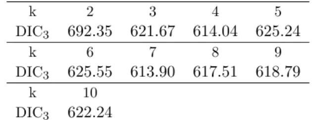
In table 1 we show the DIC3 values for different number of components of the mixtures (k); we
take for each computation of DIC3 20000 iterations with 10000 iterations for burn-in. A post hoc
analysis of chains did not show a significant departure from convergence. The lowest values are found for k = 4 and k = 7 with not many differences among them; in this case a slightly smaller value, 613.90, is obtained for k= 7. Observe that this result is fairly closed to the desired objective, as the simulation was based in 7 groups with different means and same variance.
k 2 3 4 5 DIC3 692.35 621.67 614.04 625.24 k 6 7 8 9 DIC3 625.55 613.90 617.51 618.79 k 10 DIC3 622.24
Table 1: Values of DIC3 fork components of mixtures
We consider, therefore, the analysis of a mixture model withk= 7 elements. Results show a good behaviour, as the estimated probability of type I error is only 0.02, namely, only a 2% of all hypotheses are rejected being true. By the other hand, we have an estimated value of the false discovery rate (FDR) of 0.025, namely, only a 2.5% of those hypotheses that are true, are rejected. We also have obtained that no one of hypotheses are accepted being false, but among them, 4% of hypotheses being false are classified with a different mean than those that were simulated from. The mixture of non-central t-distributions, which corresponds to the distribution of the statistics that we defined, fits correctly the simulated data. Moreover, with this approach we can consider at the same time different groups of genes in order to make multiple comparisons.
4.2 An application in Bioinformatics
Once we have checked the procedure with simulated data, we consider an application in Bioinformatics. We take data from a microarray experiment with human (Homo sapiens), bonobo (Pan paniscus) and gorilla (Gorilla gorilla) cultured fibroblasts done by Karaman et al. (2003). Expressions profiles are obtained by means of Affymetrix HG U95Av2 chips for 12625 genes in 46 samples (23 humans, 11 bonobos and 12 gorillas), and they are available in the Bioconductor libraryfibroEset(see Gentleman et al. (2004)). In order to study genes with relevant effects, we select 95 genes whose expression scores are greater or equal than 6000.
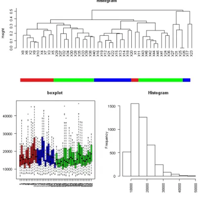
As a first step, we consider a glance at the data by means of the package made4 (Culhane et al. (2005)), from theBioconductor bundle. We show a dendrogram with a hierarchical cluster analysis (based on a Pearson correlation distance metric with average linkage) of the 46 individuals, a boxplot and a histogram of the data.
In figure 1, red color corresponds to bonobos, green color corresponds to humans and blue color to gorillas. Apparently there is a slightly more proximity between bonobos and humans than in the case of gorillas. This is coherent with the evolutionary origin of the three species. Having a look to the boxplot it shows that sample variances are roughly equal for the three species, although distribution of data are far from a single distribution. The histogram shows an asymmetric distribution of data; therefore, as the original data were originally re-normalized by Karaman et al. (2003), they correspond to the three population normal distributions of the expressions of genes.
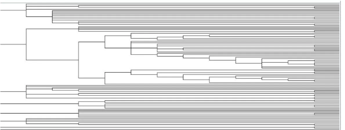
In order to have a look to the number of possible groups included in data, we apply a hybrid
clustering method,HOPACH (Hierarchical Ordered Partitioning And Collapsing Hybrid), which is a popular technique used in Bioinformatics. It builds a hierarchical tree of clusters using partitioning and agglomerative methods (see van der Laan and Pollard (2003)). We obtain the following dendrogram, that suggests about 7 main clusters.
Now, we consider a mixture of non-central t-distributions with an unknown number of components. Although in figure 2 it is suggested about 7 clusters we compute also the DIC3 values for different
number of components k, which are shown in table 2. Results are obtained after a total of 20000 iterations with 10000 iterations for burn-in. The lowest value, 1438.83, is obtained fork= 6. We also considered apost hoc analysis of chains which did not show a significant departure from convergence.
Figure 1: Overview of data: dendrogram with average linkage clustering, boxplot and histogram. k 2 3 4 5 DIC3 1602.50 1536.20 1478.37 1465.82 k 6 7 8 9 DIC3 1438.83 1454.75 1457.89 1450.32 k 10 DIC3 1468.37
Table 2: Values of DIC3 with respect tok
We consider, therefore, the analysis of a mixture model with k = 6 elements. The posterior distribution of the means (δj,j= 1, . . .6) of each component of the mixture are shown in table 3.
mean sd HPD 2.5% Median HPD 97.5% µ1 2872.6 620 880 2930 3880 µ2 3754.5 700 2700 3670 5230 µ3 4534.1 780 3270 4420 6540 µ4 5539.3 980 4050 5460 7200 µ5 7070.0 2820 4650 6600 12870 µ6 19884.4 30250 5880 10060 79020
Table 3: Posterior distribution of means of the six components of the mixture
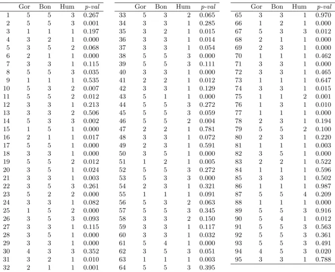
Based on previous clusters, we can propose the classification of each T statistic, based on the criterion presented in section 3 as the rule of classification. Results are shown in table 4.
We deal, as an indirect way to validate the results, with 95 independent ANOVAs which are computed gene by gene. Direct comparison of results is not possible as ANOVAs do not take into
Figure 2: Dendogram using HOPACH.
account the conjoint relations among genes. We show the corresponding p-values of the tests in the last column of table 4. In terms of hypothesis testing, the decisions with respect to equality of the 95 genes are similar between ANOVAs and mixture of t-distributions method, although the independent ANOVAs tend to accept the hypotheses of equality among genes more frequently than the mixture of t-distribution method.
It is observed that the statistics show a closer relationship between human and bonobos than respective to gorillas; this fact is supported by the evolutionary relationships among the three species. Anyway, deeper insights on a pure genetic interpretation of results obtained in these particular data are beyond the scope of this paper.
Gor Bon Hum p-val 1 5 5 3 0.267 2 5 5 3 0.001 3 1 1 1 0.197 4 3 2 1 0.000 5 3 5 2 0.068 6 2 1 1 0.000 7 3 3 1 0.115 8 5 5 3 0.035 9 1 1 1 0.535 10 5 3 2 0.007 11 5 5 2 0.012 12 3 3 1 0.213 13 3 3 2 0.506 14 5 3 3 0.002 15 1 5 1 0.000 16 2 1 1 0.017 17 5 5 1 0.000 18 3 3 1 0.000 19 5 5 2 0.012 20 3 5 1 0.024 21 3 3 1 0.003 22 3 5 3 0.261 23 5 2 2 0.000 24 3 3 1 0.082 25 1 5 2 0.000 26 3 5 3 0.093 27 3 3 1 0.115 28 3 5 1 0.000 29 3 3 1 0.000 30 4 3 3 0.352 31 3 2 1 0.010 32 2 1 1 0.001
Gor Bon Hum p-val
33 5 3 2 0.065 34 3 3 1 0.285 35 3 2 1 0.015 36 3 3 1 0.014 37 3 3 1 0.054 38 5 5 3 0.000 39 5 5 3 0.111 40 3 3 1 0.000 41 2 2 1 0.012 42 3 3 1 0.129 43 5 1 1 0.000 44 5 5 3 0.272 45 5 5 3 0.059 46 5 5 2 0.004 47 2 2 1 0.781 48 3 3 1 0.072 49 2 3 1 0.591 50 3 5 1 0.000 51 1 2 1 0.005 52 5 5 3 0.272 53 5 3 3 0.000 54 2 3 1 0.321 55 1 1 1 0.091 56 5 3 2 0.063 57 5 5 3 0.345 58 3 3 2 0.150 59 3 3 1 0.117 60 3 3 1 0.032 61 5 4 1 0.000 62 3 5 3 0.051 63 1 1 1 0.003 64 5 5 3 0.395
Gor Bon Hum p-val
65 3 3 1 0.970 66 1 2 1 0.000 67 5 3 3 0.012 68 2 1 1 0.000 69 2 3 1 0.000 70 1 1 1 0.462 71 3 3 1 0.000 72 3 3 1 0.465 73 1 1 1 0.647 74 3 3 1 0.015 75 1 1 2 0.001 76 1 3 1 0.010 77 1 1 1 0.000 78 2 3 1 0.194 79 5 5 2 0.100 80 2 3 1 0.220 81 1 1 1 0.003 82 3 5 1 0.000 83 2 2 1 0.522 84 1 1 1 0.596 85 3 3 1 0.502 86 1 1 1 0.987 87 5 5 4 0.209 88 1 1 1 0.000 89 5 5 3 0.916 90 5 4 1 0.012 91 5 5 3 0.563 92 5 5 3 0.361 93 5 5 3 0.491 94 4 5 3 0.020 95 3 3 1 0.788
Table 4: Classification of statistics in the defined groups
5
Conclussions
In this paper we have shown a methodology that is well adapted to multiple hypothesis testing prob-lems, based on a clustering methodology in Bioinformatics. With this approach, it is possible to tackle with multiple comparisons among more than two groups of different microarray expressions of genes. All groups can be analysed at the same time, and it is not necessary to compare them by pairs, as it is done in the standard post hoc analysis of multiple comparisons analysis.
Observe that original data are assumed to be normally distributed, although this is an usual assumption in microarray analysis, after standard procedures of normalization and data cleaning. Then, a mixture of non-central t-distributions is straightforwardly obtained when we define a standard statistic (denoted byT). This is related only with the sample means and variances of groups of data; namely, there are not other guesses in our model but normality of data, and computation of sample means and sample variances.
By the other hand, the results obtained with simulated data are adequate, and the analysis of real data renders sensible conclusions in the line of other standard methods of clustering or multiple testing techniques used in Bioinformatics.
References
G. Celeux , F. Forbes, C. P. Robert and D. M. Titterington (2006). Deviance Information Criteria for Missing Data Models. Bayesian Analysis 1(4), 651–674.
S. T. B. Choy and A. E. M. Smith (1997). Hierarchical Models with Scale Mixtures of Normal Distri-butions. TEST 6(1), 205–221.
A. C. Culhane, J. Thioulouse, G. Perriere and D. G. Higgins (2005). MADE4: an R package for multivariate analysis of gene expression data.Bioinformatics 21(11), 2789–2790.
D. B. Dahl and M. A. Newton (2007). Multiple Hypothesis Testing by Clustering Treatment Effects.
JASA 102478, 517–526.
D. B. Dahl, Q. Mo and M. Vannucci (2008). Simultaneous inference for multiple testing and clustering via a Dirichlet process mixture model. Statistical Modelling 8(1), 23–39.
S. Dudoit, J. P. Shaffer and J. C. Boldrick (2003). Multiple Hypothesis Testing in Microarray Exper-iments. Statistical Science 18(1), 71–103.
R. Gentleman, V. Carey, D. Bates, B. Bolstad, M. Dettling, S. Dudoit, B. Ellis, L. Gautier, Y. Ge, J. Gentry, K. Hornik, T. Hothorn, W. Huber, S. Iacus, R. Irizarryand, F. Leisch, C. Li, M. Maechler, A. Rossiniand, G. Sawitzki, C. Smith, G. Smyth, L. Tierneyand, J. Yang and J. Zhang, (2004). Bioconductor: Open software development for computational biology and bioinformatics. Genome Biology 5, R80.
http://www.bioconductor.org.
P. Green (1995). Reversible jump MCMC computation and Bayesian model determination.Biometrika 82, 711–732.
Y. Ji, Y. Lu and G. B. Mills (2008). Bayesian models based on test statistics for multiple hypothesis testing problems. Bioinformatics 24(7), 943–949.
N. L. Johnson, S. Kotz and N. Balakrishnan (1995).Continuous Univariate Distributions Volume 2. Wiley & Sons, New York.
M. W. Karaman, M. L. Houck, L. G. Chemnick, S. Nagpal, D. Chawannakul, D. Sudano, B. L. Pike, V. V. Ho, O. A. Ryder, and J. G. Hacia (2003). Comparative Analysis of Gene-Expression Patterns in Human and African Great Ape Cultured Fibroblasts.Genome Research 13, 1619–1630.
M. van der Laan and K. Pollard (2003). A new algorithm for hybrid hierarchical clustering with visualization and the bootstrap.J. of Statistical Planning and Inference 117, 275–303.
J. M. Marin and C. P. Robert (2007).Bayesian Core: A Practical Approach to Computational Bayesian Statistics. Springer, New York.
G. J. McLachlan, R. W. Bean and D. Peel (2002). A mixture model-based approach to the clustering of microarray expression data.Bioinformatics 18(3), 413–422.
M. Medvedovic and S. Sivaganesan (2002). Bayesian infinite mixture model based clustering of gene expression profiles. Bioinformatics 18(9), 1194–1206.
M. A. Newton A. Noueiry D. Sarkar and P. Ahlquist (2004). Detecting differential gene expression with a semiparametric hierarchical mixture method.Biostatistics 5(2), 155–176.
M. Plummer (2003). JAGS: A program for analysis of Bayesian graphical models using Gibbs sampling.
DSC 2003 Working Papers
http://www-fis.iarc.fr/∼martyn/software/jags/
S. Richardson and P. Green (1997). On Bayesian analysis of mixtures with an unknown number of components. J. Royal Statist. Soc. B 59, 731–792.
S. Richardson (2002). Discussion of Spiegelhalter et al.J. of the Royal Statist. Soc. B 631.
E. G. Tsionas (2002). Bayesian Inference in the Noncentral Student-t Model.J. of Computational and Graphical Statistics 11(1), 208–221.
M. Yuan and C. Kendziorski (2006). A Unified Approach for Simultaneous Gene Clustering and Differential Expression Identification. Biometrics 62, 1089–1098.