Imprecise Statistical Methods for Accelerated Life Testing

(1)

Durham E-Theses

Imprecise Statistical Methods for Accelerated Life

Testing

AHMADINI, ABDULLAH,ALI,H

How to cite:

AHMADINI, ABDULLAH,ALI,H (2019) Imprecise Statistical Methods for Accelerated Life Testing, Durham theses, Durham University. Available at Durham E-Theses Online:

http://etheses.dur.ac.uk/13053/

Use policy

The full-text may be used and/or reproduced, and given to third parties in any format or medium, without prior permission or charge, for personal research or study, educational, or not-for-prot purposes provided that:

• a full bibliographic reference is made to the original source

• alinkis made to the metadata record in Durham E-Theses

• the full-text is not changed in any way

The full-text must not be sold in any format or medium without the formal permission of the copyright holders. Please consult thefull Durham E-Theses policyfor further details.

(2)

Academic Support Oce, Durham University, University Oce, Old Elvet, Durham DH1 3HP e-mail: [email protected] Tel: +44 0191 334 6107

http://etheses.dur.ac.uk

(3)

Imprecise Statistical Methods for

Accelerated Life Testing

Abdullah Ali H. Ahmadini

A Thesis presented for the degree of

Doctor of Philosophy

Statistics and Probability

Department of Mathematical Sciences

University of Durham

England

April 2019

(4)

Dedicated to

To Allah my God. To my father and mother.

(5)

Imprecise statistical methods for

accelerated life testing

Abdullah Ali H. Ahmadini

Submitted for the degree of Doctor of Philosophy

April 2019

Abstract

Accelerated Life Testing (ALT) is frequently used to obtain information on the lifespan of devices. Testing items under normal conditions can require a great deal of time and expense. To determine the reliability of devices in a shorter period of time, and with lower costs, ALT can often be used. In ALT, a unit is tested under levels of physical stress (e.g. temperature, voltage, or pressure) greater than the unit will experience under normal operating conditions. Using this method, units tend to fail more quickly, requiring statistical inference about the lifetime of the units under normal conditions via extrapolation based on an ALT model.

This thesis presents a novel method for statistical inference based on ALT data. The method quantifies uncertainty using imprecise probabilities, in particular it uses Nonparametric Predictive Inference (NPI) at the normal stress level, combin-ing data from tests at that level with data from higher stress levels which have been transformed to the normal stress level. This has been achieved by assuming an ALT model, with the relation between different stress levels modelled by a sim-ple parametric link function. We derive an interval for the parameter of this link function, based on the application of classical hypothesis tests and the idea that, if data from a higher stress level are transformed to the normal stress level, then these transformed data and the original data from the normal stress level should not be distinguishable. In this thesis we consider two scenarios of the methods. First, we present this approach with the assumption of Weibull failure time distributions at each stress level using the likelihood ratio test to obtain the interval for the

(6)

pa-iv

rameter of the link function. Secondly, we present this method without an assumed parametric distribution at each stress level, and using a nonparametric hypothesis test to obtain the interval.

To illustrate the possible use of our new statistical method for ALT data, we present an application to support decisions on warranties. A warranty is a con-tractual commitment between consumer and producer, in which the latter provides post-sale services in case of product failure. We will consider pricing basic warranty contracts based on the information from ALT data and the use of our novel imprecise probabilistic statistical method.

(7)

Declaration

The work in this thesis is based on research carried out in the Department of Math-ematical Sciences at Durham University. No part of this thesis has been submitted elsewhere for any degree or qualification.

Copyright c 2019 Abdullah Ali H. Ahmadini.

“The copyright of this thesis rests with the author. No quotations from it should be published without the author’s prior written consent and information derived from it should be acknowledged”.

(8)

Acknowledgements

Alhamdullilah, first and foremost. I am truly grateful to Allah my God for the countless blessings He has bestowed on me, both generally and in accomplishing this thesis especially. I would like to express my warmest gratitude and deepest appreciation to my academic supervisor, Professor Frank Coolen, for his untiring support, patience, kindness, enthusiasm, calm advice, suggestions with immense knowledge, and guidance throughout my work and during the writing of this thesis. He is a very supportive, nice person, who has very much helped and supported me during my stay in Durham. Whilst Professor Frank has been like a second father to me, he has also always listened to me and respected my situation when my wife and my son were far away. I will not forget his help and encouragement which will have a significant impact on my future. Also, I would like to thank Dr. Tahani Coolen-Maturi for her ideas and support with my computational and research questions.

I am truly grateful to my father and my mother who have been a great source of motivation, constant support, love, and prayers, and have always stood by me and been proud of me. I would like to express my sincere gratitude to my brothers and sisters for their confidence, encouragement, and helping my wife and my son for all their needs while I have been abroad.

Special thanks and warm appreciation also go to my beloved wife Reem Ahmadini for her patience, love, prayers, standing by me, her kindness, and taking care of our son Mohammed while I was abroad. Thanks to my son Mohammed.

I gratefully acknowledge the financial support from Jazan University in Saudi Arabia and the Saudi Arabian Cultural Bureau (SACB) in London to allow me to pursue my PhD studies at Durham University.

Many thanks also to Durham University for providing me with an enjoyable vi

(9)

vii

academic atmosphere, for offering me great opportunities to participate and present my results at international conferences, and for the facilities that have enabled me to study comfortably.

Finally, many thanks go to my colleagues, friends, and to everyone who has assisted me, stood by me or contributed to my educational progress in any way.

(10)

Chapter 1 Introduction

The aim of accelerated life testing (ALT) is to allow researchers to estimate the useful lifespans of products or components and to inform advances in product reliability [50, 60]. The unique characteristic of ALT is to determine the reliability of products in a shorter period of time. The process of testing components’ expected lifespans under normal operational conditions may be time-consuming and expensive. ALT is frequently used to determine the reliability level of devices in a shorter period of time. The basic premise of ALT is to test a unit under greater-stress conditions than the stress levels encountered under normal usage. ALT represents an important technique for gathering product failure information under a variety of conditions within a reasonable time and budget [50, 60].

In this thesis, we present a new imprecise statistical inference method for ALT data, where nonparametric predictive inferences (NPI) at normal stress levels are integrated with a parametric link function, combining data from tests at that level with data from higher stress levels which have been transformed to the normal stress level. The method includes imprecision which provides robustness with regard to the model assumptions. The imprecision leads to observations at increased stress levels being transformed into interval-valued observations at the normal stress level, where the width of an interval is larger for observations from higher stress levels.

Generally, uncertainty, within the field of statistics and probability, tends to be measured by classical probability following Kolmogorov’s axioms [12]. Generalisa-tion of Kolmogorov’s axioms can bring forth possible soluGeneralisa-tions when informaGeneralisa-tion

(13)

1.1. Motivation 2

and knowledge are limited or incomplete, where classical probability is considered too restrictive [12]. Such generalisation includes the use of imprecise probabilities, which is mainly characterized by using lower and upper bounds for probabilities instead of the standard theory of ‘precise’ or ‘single valued’ probability [8, 12, 70]. Further, the domain of imprecise probability, which has seen a wealth of research over the past two decades, has served as a motivation to researchers in various areas of statistics and engineering. This has resulted in a project website (The Society for Imprecise Probability: Theories and Applications - www.sipta.org) and biennial conferences [8, 48].

Over recent years, a number of methods of quantifying uncertainty and assessing reliability have appeared in the literature, which provide many benefits compared to classical probability. Thus, these methods and their respective practical appli-cations represent a key area of cutting-edge research in this domain. For instance, interval probability [74, 75] and the theory of imprecise probabilities [72] provide techniques for reliability analysis. Regarding imprecise probabilties, Coolen [20] has investigated a range of problems related to imprecise reliability by assessing various tools designed to apply imprecise reliability to many practical applications.

The interesting work on imprecise probability has paved the road to the devel-opment of new methods of statistical inference such as nonparametric predictive inference (NPI) [9]. Many researchers have presented applications of NPI related to new approaches on different types of data.

The rest of this chapter is organized as follows. Section 1.1 provides the mo-tivation for the work in this thesis. In Section 1.2, we provide the outline of this thesis.

1.1 Motivation

Because of the complex nature of ALT scenarios, there can be quite complicated modelling for statistical inference, which provides many challenges. Thus, the main object of this thesis is to provide a straightforward, robust model for quantifying imprecision in which can be widely used in practical applications. This model will

(14)

1.1. Motivation 3

generate interval-based probabilities rather than exact probabilities. However, if these interval-based data fail to provide clear insight into ways to overcome practical application issues, we can modify our model’s assumptions, collect more data or include specialist opinion to refine our approach. The starting point of this work is that the paper of Yin et al. [79], where it was first suggested.

Yin et al. [79] introduced an imprecise statistical method for ALT data using the power-Weibull model. In their paper, they developed the imprecision in the power-law link function by considering an interval around the parameter estimate, leading observations at stress levels other than the normal level to be transformed into intervals at the normal level [79]. Yin et al. [79] did not give an argument, other than simulation studies, for the amount of imprecision in the parameter. Building on the work by Yin et al. [79], we introduce the use of classical statistical tests between pairwise stress levels to obtain the interval for the parameter of the link function. This use of frequentist statistical tests to determine the level of imprecision is the main contribution presented in this thesis.

We obtain an interval for the parameter of the link function which is assumed at each stress level by (i) applying classical hypothesis testing between the pairwise stress levels to determine the level of imprecision, and (ii) assuming that if data from a higher stress level are then transformed to a normal stress level, then the transformed data and the original data (i.e. from the normal stress level) should, in theory, be indistinguishable. Note that each observation at the higher stress level is transformed to an interval at the normal stress level, where the interval tends to be larger if a data point was originally derived from a higher stress level.

We present this method using the assumption of Weibull failure time distribu-tions at each stress level using the likelihood ratio test to obtain the interval; as well as without such an assumption, but using a nonparametric hypothesis test to obtain such interval for the parameter of the link function. We explore impreci-sion in the link function, which will allow observations of increased stress levels to be transformed to interval-valued observations at normal stress levels. We then present simulation studies to investigate the performance of the proposed method to establish appropriate links between stress test levels.

(15)

1.2. Outline of the thesis 4

1.2 Outline of the thesis

In this thesis, we develop novel important extensions for the use of the imprecise statistical predictive inference method for accelerated life testing data. Our new approach provides robustness for the predictive inference by using statistical tests between the pairwise stress levels, to obtain the intervals for the values of the pa-rameter of the link function. Thus, this thesis provides an innovative approach by using frequentist statistical tests to determine the level of imprecision.

This thesis is structured as follows. Chapter 2 introduces and summarizes key background concepts from the literature, applicable to the topics investigated in this thesis. It provides a brief overview of the ALT concepts and some of the life distribution functions which are applicable in reliability applications. We briefly discuss stress loading methods which can be applied in accelerated testing, including constant, step, and progressive stress loading. Chapter 2 also briefly review the statistical tests which are used in the thesis. Then, we address general notions of imprecise probability and the main idea of nonparametric predictive inference (NPI). In Chapter 3, we present a new predictive inference method based on ALT data and the likelihood ratio test. It assumes a failure time distribution with a parametric link function at each stress level. We apply the pairwise likelihood ratio test to create an interval for the parameter of the link function. We assume a distribution model for all levels and derive an interval for the parameter of the link function using pairwise likelihood ratio tests. We use this interval to transform observations of increased stress levels to interval-valued observations at the normal stress level.

Also, we use NPI at the normal stress level to achieve predictive inference on the failure time of a particular unit operating under normal stress levels using the original data at the normal stress level and interval-valued data transformed from higher stress levels. We investigate the performance of our method via simulations. A paper presenting the results in this chapter has been submitted for publication [6]. Also, the results of this chapter have been presented at several seminars and con-ferences, and we have also published short papers in related conference proceedings. Parts of Chapter 3 have been presented at the 2017 Research Students’ Confer-ence in Probability and Statistics at the University of Durham, and at the 10th

(16)

1.2. Outline of the thesis 5

IMA International Conference on Modelling in Industrial Maintenance and Reliabil-ity (Manchester, 2018), and a related short paper was published in the conference proceedings [3]. The results of Chapter 3 have also been presented at the 3rd In-ternational Conference on System Reliability and Safety (Barcelona, 2018), and a related short paper was published in the conference proceedings [5].

Chapter 4, presents a similar method to in Chapter 3 but without the assump-tion of a parametric distribuassump-tion for the failure times at each stress level. The method is largely nonparametric, with a basic parametric function to link different stress levels. We use the log-rank test to provide adequate imprecision for the link function parameter, and conduct simulation studies to investigate the performance of our proposed approach. A paper based on this chapter has been submitted for publication [26]. This was presented at the Soft Methods in Probability and Statis-tics (SMPS) conference (Compigne, 2018), and a short paper was published in the conference proceedings [4].

In Chapter 5 we explore the use of our new methods, as presented in Chapters 3 and 4, for decision making with regard to warranties. This work will be presented at the ESREL conference (Hannover, 2019), a short paper has been submited for the conference proceedings [7].

(17)

Chapter 2 Background

This chapter provides an overview of concepts from the literature relevant to the topics investigated in this thesis. Section 2.1 present an overview of reliability test-ing. Section 2.2 provides a brief introduction to the main concepts of accelerated life testing (ALT). We present a brief overview of ALT and discuss some of the commonly used failure distributions and ALT link functions between stress levels. In Section 2.3, we briefly review basic statistical tests used in this thesis, namely the likelihood ratio test and the log-rank test. The likelihood ratio test and log-rank test will be employed in Chapters 3 and 4, respectively. Finally, we give an overview of the main aspects of NPI in Section 2.4.

2.1 Reliability testing

Reliability analysis techniques play an important role in the engineering field and the manufacturing industry in terms of product design and development processes. How-ever, product reliability analysis is renowned for being a time-consuming process. Reliability analysis is used to model a product’s time to failure in most applications, and falls into two categories: complete (where all failure data are made available) and censored (where some data are omitted) [41, 60].

In terms of complete data sets, exact test-unit failure times are used, as these data are both measured and known [41, 60]. However, not all (or indeed any) units may fail during a single testing cycle; such data are called censored data [41, 60].

(18)

2.1. Reliability testing 7

Thus, because of these two different conditions under which censoring may occur, such data can be further divided into time-censored data (type I-censored) and failure-censored data (type II-censored). Type I-censored data is typically obtained when the censoring time is pre-set, and the number of failures is expressed as a random variable. In terms of type II-censored data, testing is completed following a pre-specified number of failures [41, 60]. In this case, the time period in which a specified number of failures will occur is expressed as a random variable [60].

Reliability analysis for any new product at time t = 0 and consequent failure at timeT employs two terms: the reliability function R(t) and the hazard function

h(t), where T represents the reliability period for the product in question [41]. The reliability functionR(t) represents the probability that the product will survive until time t. It is defined as

R(t) =P(T > t) = 1−F(t). (2.1.1) Note that the reliability functionR(t) is a monotonically decreasing function:

R(t1)≥R(t2)∀t1 < t2. (2.1.2) whereR(0) =P(T > 0) = 1.

A concise definition of the hazard rate is the immediate potential per unit time for an event to occur based on the assumption that an individual unit has withstood testing up until time t [41]. This results from the determination of the survival function, because when t increases, the survival rate will never increase [41]. The hazard function h(t) is defined as

h(t) = lim

4t→0

P(t ≤T < t+4t|T ≥t)

4t . (2.1.3)

Maximum likelihood estimation (MLE) is a well-known and widely used statisti-cal method used to estimate the parameters of probability distributions. Likelihood functions are formed from observed data and the chosen distribution for these data, which are assumed to be independent and identically distributed [1, 60, 62]. The likelihood function has been discussed a great deal in the literature, and applied to both failure data and censored data [60].

(19)

2.2. Accelerated life testing 8

The method of MLE can be used for estimating the unknown parameters of lifetime distributions. The likelihood function for a chosen failure time distribution with parameterθ is defined as

L(θ;t) = n Y i=1 f(ti;θ) u Y j=1 S(cj;θ),

where f(.) is the probability density function, ti is the observed failure times, and

i= 1, ..., n. S(.) is the survival function, cj is the censored times, and j = 1, ..., u.

When assessing the reliability of a new product, the foremost challenge is to determine reliability in a relatively short period of time. Typically, we use lifes-pan to assess a product, system or component. In traditional testing methods, researchers perform these life tests only under normal operating conditions, to di-rectly determine a product’s failure time distribution and the parameters associated with failure. However, this method of obtaining life data at least in its current form is often not viable in present-day industrial testing because current products are typically more reliable than in the past. Further, there are also greater time pres-sures nowadays where new products are required to be launch-ready very soon after they have been designed. This issue has provided the motivation to create a new lifespan testing method, namely accelerated life testing (ALT), which can provide meaningful product failure data in a short space of time. ALT will be introduced in the next section.

2.2 Accelerated life testing

ALT is frequently used to gather information on the expected lifespans of a range of devices; it represents an efficient way of testing, if testing under normal conditions requires a great deal of time and expense. Thus, ALT enables testing the reliability of devices in shorter time periods and at lower cost. ALT involves testing a particular unit under varying degrees of physical stress (e.g. temperature, voltage, or pressure), greater than normal operating conditions. This approach causes devices to tend to fail more quickly, enabling testers to estimate devices’ expected lifetimes under normal operating conditions via extrapolation using an ALT model.

(20)

In recent decades, various methods for analyzing ALT data and a variety of meth-ods for assessing the reliability with different ALT scenarios have been introduced. An excellent introduction to ALT was given by Nelson [60]. This was followed by a large literature on ALT. In what follows, we we briefly introduce some designs of ALT tests, life time distribution, and acceleration models [60].

A wide range of test designs can be applied in accelerated testing, the main ones are: constant-, step- and progressive-stress testing [60]. The basis for classification of the stress loading is the dependency of the stress with respect to time t.

Constant stress loading (which is time-independent) is the most common form of stress loading, where products operate at constant stresses. In constant-stress testing, units are tested at a specific stress levelK0, K1, ..., Km until they either fail

at that particular stress level or testing is ended for another reason [60].

Constant stress loading has several advantages [60]. When the experiment is designed, extrapolation at the constant use level condition is more accurate than time-varying loading. This is because all units under constant stress are maintained at the same voltage, temperature, or pressure for a given stress level, which makes it easier and simpler to run each test. However, the failure of units under constant stress usually takes a long time, especially at normal levels of stress, which makes it more time-consuming than testing under time-dependent stress levels [60]. We only consider the constant stress loading in this thesis, because it is the simplest stress loading for which to develop new methods. Note that we do not consider design of ALT tests in this thesis, we just assume the data are given.

When developing an acceleration model, to determine the life-stress relationship in ALT, two important components need to be considered. First, we need to describe the relationship between failure time and stress level. In particular, they should reflect the way that various levels of stress affect how quickly the failure mechanisms occur, and how stress affects the overall lifetime of a given device. In real life if one increases the stress, the failure occurs faster, and it may lead to different modes of failure that would need to be modelled. However, in this thesis, we assume that the modes of failure and their relative frequency are unchanged by stress and we only study the statistical development of the methods. The model should also include a

(21)

lifetime distribution for each fixed stress level (e.g. Weibull or log-normal) [50, 60]. Variations among products, in terms of performance, lifetime and quality, can be modelled by a statistical distribution. Life time distribution functions describe distributions for products which are applicable to failure data analysis and relia-bility estimations [60]. Life time distributions can be used to model increasing or decreasing failure rate, and analyse the differences between the products, and to model reliability [50, 60]. One of the most commonly used and widely applicable distributions used for life data analysis is the Weibull distribution, which we use in this thesis.

The Weibull distribution [60] is a popular way to model reliability, and is thus used for examining product lifetime. It is also used to describe the failure properties of electronic components and the breaking strengths of the material(s) they are composed of [60]. Breaking strengths (electronical or mechanical) in accelerated test form one example [60]. The Weibull distribution is commonly utilised in the accelerated testing of roller bearings [50, 60]. The Weibull distribution [60], is given by f(t) = β α( t α) β−1_exph₋₍t α) βi_,

where t > 0. The unknown parameters of the Weibull distribution are the shape parameterβ > 0, and the scale parameter α >0 , and its survival function is

S(t) = exph−t

α

βi

.

The hazard rate of the Weibull distribution is

h(t) = f(t)/S(t) = β α t α β−1 ,

where the h(t) is the hazard rate at age t. In short, the hazard rate is used to discribe whether the failure rate of a product increases or decreases with product age [60]. For β > 1, the hazard rate is a strictly increasing function with respect to time and when β < 1, the Weibull distribution shows a decreasing hazard rate.

(22)

Forβ = 1, the Weibull distribution has a constant hazard rate and is equal to the Exponential distribution [50, 60]

Some other distributions used for life data analysis are the Exponential, Log-normal, and Gamma distributions, but we do not consider these in this thesis. Note that they can be used instead of the Weibull distribution in Chapter 3, as long as these would be combined with a link function such that it enables transformation as has been done in Chapter 3.

Determining the life-stress relationship in ALT usually involves using either a physical or an empirical acceleration model [68]. Physical or chemical theory based models are attractive for some failure mechanisms [68]. These types of models de-scribe the process that causes device failure over a range of stress levels, in order to facilitate extrapolation to the normal stress level [68]. Failure mechanisms and accelerating variables usually have a complicated relationship [68]. In most situa-tions, a simple model will not be sufficient to describe the failure process and its causes [50, 60, 68].

In this thesis, we do not aim at complex models but we are exploring simple models combined with imprecision to get robustness around the simple models. We have not found such an ALT method combined with imprecise probability methods in the literature. Statistical inference for ALT data tends to focus on parameter estimates. We comment on this in Chapter 6.

ALT is used for extrapolating information to the normal stress level about fail-ure time distributions, and the reliability of a given product [60, 68]. Acceleration factors are used to determine the failure time at a particular stress level, which can subsequently be used to predict the failure time at different levels of operating stress [60,68]. This is known as an acceleration model. While statistical distributions identify the lifetimes of a particular type of unit at each stress level and distribution for items, the acceleration model derives the scale parameter, or the shape parame-ter of a life distribution, as a function of the applied stress [50, 60, 68]. Some of the most important and commonly used acceleration models are the Arrhenius, Eyring,

(23)

and power-law models, which we use in this thesis [17, 34, 50, 60, 71].

The Arrhenius life-stress relationship model is one of the most widely used for testing when the stimulus or accelerated variable is thermal stress [60, 68]. It is often an appropriate choice if a unit’s failure mechanism is driven by temperature [60, 68]. The physics-based Arrhenius law for chemical reaction rates explains that as temperature increases, this induces increased levels of atomic movement, and so the processes that cause failure speed up [60, 68]. Therefore, the Arrhenius model explains the reaction rate α of a unit as a function of applied temperature [17, 34, 50, 60, 71]. This model can be expressed as

α=Aexp −EA kB.K , (2.2.1)

where α is the reaction rate, A is a constant characteristic of the united failure mechanism and test condition, EA is the activation energy in electron-volts, kB

is the Boltzmann’s constant (8.6171×10−5 _{electron-volts per} ◦_C_{), and} _K _{is the}

absolute temperature (Kelvin) for the Arrhenius relationship (accelerated stress). By taking the natural logarithm of (2.2.1), it yields the linear relationship

ln(α) = γ0+

γ

K, (2.2.2)

whereγ = EA

kB, γ0 = ln(A).

The natural logarithm of the scale parameter at the normal stress level is

ln(α0) =γ0+

γ K0

,

and the natural logarithm of the scale parameter at the higher stress level is

ln(αi) =γ0+

γ Ki

.

The Weibull distributions for different stress levels are assumed to have different scale parametersαi >0 for leveli. The Arrhenius link function for scale parameters

(24)

2.2. Accelerated life testing 13 αi =α0exp γ Ki − γ K0 . (2.2.3)

Where using this model with temperature as stress levels, K0 is the normal temperature (Kelvin) at stress level 0, Ki is the higher temperature (Kelvin) at

stress level i, and γ >0 is the parameter of the Arrhenius link function model. In this thesis, we use the Arrhenius model under the Weibull distribution to link the scale parameter at different failure times. The Arrhenius model, however, can-not be applied to all temperature issues [60, 68]. In some cases, it is sufficient over only a limited temperature range [60, 68]. According to Nelson [60], in particular real-world application (e.g. motor insulation), the Arrhenius model may not fit the data well [60].

The Eyring model provides an alternative to the Arrhenius model. It also uses temperature as the accelerating variable, and is based on quantum mechanics [50,60, 71]. In this model, the relationship between mean time to failureαand temperature

K is defined by α= A K exp( λ K), whereλ= EA

kB. A and λ >0 are constant characteristic of the united failure mecha-nism and test condition,kBis the Boltzmann’s constant, (8.6171×10−5electron-volts

per◦C), and K is the absolute temperature (Kelvin).

The scale parameter of a unit at the normal stress level is

α0 = A K0 exp( λ K0 ),

and the scale parameter at the higher stress level is

αi = A Ki exp( λ Ki ). (2.2.4)

(25)

The Eyring link function for the Weibull scale parameters is

αi =α0×(K0/Ki)×exp

h

(λ/Ki−λ/K0)

i

Where using this model with temperatures as stress levels, K0 is the normal temperature (Kelvin) at stress level 0, Ki is the higher temperature (Kelvin) at

stress level i, and λ >0 is the parameter of the Eyring link function model.

The Eyring model can be applied to testing capacitors, electro-migration failure, and solid rupturing [60]. It should be noted that both the Eyring and Arrhenius models derive similar results in many applications, and both fit failure times related to temperature [60].

The power-law model is commonly used for testing when the stimulus or accel-erated variable is voltage stress. It is often an appropriate choice if a unit’s failure mechanism is driven by voltage to analyse lifetime data as a function of the ALT model [60]. In the power-law model, the relationship between scale parameterαand voltageK is

α= 1 (C.K)γ,

where C and γ are parameters representing characteristics of the product and test method, andK represents the stress level in terms of voltage. The scale parameter at normal stress level is

α0 = 1 (C.K0)γ

,

and the scale parameter at the higher stress level is

αi =

1 (C.Ki)γ

.

The power-law link function of scale parameterαi should be used for establishing

a connection between different stress levelsi, and is assumed to satisfy the function

αi =α0

K₀

Ki

γ

(26)

Where using this model with different voltages as the stress levels, K0 is the normal voltage at stress level zero,Ki is the higher voltage at stress levels, andγ is

the parameter of the power-law link function model.

Some common applications of the power-law model are for testing electrical in-sulation, dielectrics in voltage endurance evaluations and materials, bearings, and electronic devices, to determine their useful lifespans and reliability [60]. For more details, see [50, 60].

As examples of applications, Fan et al. [30] presented the maximum likelihood estimation (MLE) and Bayesian inference on all parameters of ALT models under an exponential distribution, with a linear link function between the failure rate and the stress variables under the Box-Cox transformation. Fard and Li [31] presented an optimal step stress to obtain the optimal hold time at which the stress level is changed for step stress ALT design for reliability prediction. They assumed a Weibull distribution for the failure time at any constant stress level, and the scale parameter of the Weibull distribution was assumed to be a log-linear function of the stress level. Elsayed and Zhang [29] proposed an optimal multiple-stress-type ALT plan using a proportional hazards model to obtain failure time data rapidly in a short period of time. Sha and Pan [67] introduced step-stress ALT with Bayesian analysis for the Weibull proportional hazard model. Nasir and Pan [59] assumed a Bayesian optimal design criterion and presented acceleration model selection ALT studies, while Han [36] conducted research into temporally and financially constrained constant-stress and step-stress ALT.

Whilst ALT models typically consider failure times as the events of interest, there have also been important contributions with more detailed modelling, in particular exploiting methods to mathematically model degradation processes. For example, Liao and Tseng [44] proposed an optimal design for step-stress accelerated degrada-tion tests with the degradadegrada-tion process modelled as a stochastic diffusion process. Pan et al. [64] presented a bivariate constant stress accelerated degradation model and related inference. They assumed a device which has two performance charac-teristics which are modelled by a Wiener process, to determine the relibility of high

(27)

2.3. Basic Statistical Methods 16

quality devices with a time scale transformation, and the Frank copula is used to model dependence of the two performance characteristics. Duan and Wang [28] pro-posed a bivariate constant stress accelerated degradation model with inference based on the inverse Gaussian process. It is important to note here that the modelling of degradation processes does require much information about the engineering process and physical properties of the equipment, which may come from detailed measure-ments of the process or expert judgemeasure-ments. While this is an important development for real world accelerated life testing, we do not address such approaches further in this thesis and only assume information about the failure times to be present.

2.3 Basic Statistical Methods

Comparing the survival function or the probability distribution of two independent groups, possibly including right-censored observations often requires classical statis-tical tests. In this section we present a brief overview of the statisstatis-tical tests used in Chapters 3 and 4 of this thesis. Subsections 2.3.1 and 2.3.2, introduce the likelihood ratio test and the log-rank test, respectively. In Chapters 3 and 4 of this thesis, we will use these test statistics for the pairwise stress levels to find the interval of values of the parameter of the link function for which we do not reject the null hypothesis of two or more groups of failure data, possibly including right censored data, coming from the same underlying distribution. Indeed, for our methods in Chapters 3 and 4, other statistical tests could be used, and of course if we use different tests these may lead to slightly different results.

2.3.1 Likelihood ratio test

Hypothesis testing is one of the main methods in statistical inference and its appli-cations. Testing equality of the probability distribution of two or more independent groups often involves parametric statistical tests. A general classical hypothesis test that can be used to test equality of the survival distributions, is the likelihood ratio test [42, 63]. The likelihood ratio test is used to compare two independent failure data groups, possibly including right-censored observations (e.g. resulting from two

(28)

2.3. Basic Statistical Methods 17

ALT test), in assumed parametric models.

The probability density function of a statistical distribution is assumed to de-scribe the failure time at a fixed stress level, and its parameters are therefore maxi-mized in the likelihood ratio test based on the idea of hypothesis testing for which we do not reject the null hypothesis of two groups of data, coming from the same underlying distribution. To obtain the likelihood ratio test, we need to compute the difference between the log likelihood of the alternative hypothesis ˆL1 and the likelihood of the null hypothesis ˆL0 [42].

Suppose that L1 and L0 be the maximized log-likelihood under the alternative and the null hypothesis respectively. Then the likelihood ratio (LR) test statistic is

LR = 2( ˆL1 −Lˆ0), which under the null hypothesis, follows a χ2 distribution with degree of freedom which is equal to the difference in the number of parameters of each of the two models. The likelihood ratio test is discussed in more detail in all good introductory statistics books (see e.g. [42]).

2.3.2 Log-rank test

The general advantege of nonparametric tests is that they are “distribution-free”. The use of nonparametric statistical tests often involve comparison of two groups of data, e.g. data resulting from an experiment with two different groups in which units are studied in accelerated test (e.g. temperature, voltage, humidity, pressure). Test-ing equality of the survival distribution of two independent groups often involves nonparametric statistical tests. There are several nonparametric test procedures that can be used to test equality of the survival distributions. One popular non-parametric test for equality of the survival distributions of two groups is the log-rank test [46, 65]. The log-rank test is a nonparametric test and one of the most widely used for comparing the survival distribution of m ≥ 2 groups [65]. Sometimes, the log-rank test is called the Mantel-Cox test [33, 47, 66]. It compares the observed numbers of failures for two groups with the expected numbers of failures [66].

Conditionally on the number at risk in the groups [41], the log-rank test statistics can be determined by using observed and expected values for each group, and com-paring the hazard rates between the two groups throughout [65, 66]. The log-rank

(29)

2.4. Nonparametric predictive inference 18

test obtains the expected number of failure for expected number of failure for group

i∈ {1,2} as: eij = n_i,j n1,j+n2,j ×(m1,j+m1,j). (2.3.1)

Suppose that there are two groups consisting of ni (i = 1,2, ..., m) individuals.

Individuals in each group have either a failure or right-censoring time. Let 0 < t(1) < t(2) < ... < t(k) < ∞ denoted the failure time, for ease of notation let t0 = 0 and tk+1 = ∞. For ease of presentation, we assume that no ties occur among the observed value in the combined group. Suppose that m1,j denoted the number

of failures occur at tj in group one, m2,j denoted the number of failures occur at

tj in group two. Let ni,j be the number of units at risk just prior to time t(j) (j = 1,2, ..., k).

The log-rank test statistics is obtained by

log-rank= (O2−E2) 2

Var(O2−E2)

, (2.3.2)

where O2−E2 =Pk_j₌₁(m2,j−e2,j).

Therefore, the variance ofVar(Oi−Ei) is defined by

Var(Oi−Ei) = k X j=1 n1,jn2,j(m1,j+m2,j)(n1,j+n2,j−m1,j−m2,j) (n1,j+n2,j)2(n1,j+n2,j−1) . (2.3.3)

The test statistics approximately follows a χ2 _{distribution and a degree of} free-dom which is equal to the difference in the number of groups [42]. Alternative tests statistics can be used instead of the log-rank test statistics to test equality of survival functions [33].

2.4 Nonparametric predictive inference

In terms of imprecise probability, classical probability is generalised as uncertainties relating to events are measured not with single numbers but intervals [20]. For example, in classical probability, event A would be ascribed a single numberP(A)∈

(30)

[0,1], where P is a probability measured by classical probability which operates within the bounds of Kolmogorovs axioms. In terms of quantifying uncertainty, imprecise probability as a statistical concept was first proposed by Boole [15] in 1854 and has had a long history since Hampel [35]. Over the past few years, a number of alternative approaches to quantifying uncertainty have been proposed including interval probability theory, introduced by Walley [72] and Weichselberger [74] which proposes that probabilities have lower and upper range of probabilities i.e. [P(A), P(A)] respectively, with 0 ≤ P(A) ≤ P(A) ≤ 1 while classical probability theory includes a complete lack of data about the event in question i.e. P(A) = 0 and P(A) = 1. Here, P(A) represents the lower probability of event A, and

P(A) represents the upper probability for event A. The imprecision for event A is

4(A) =P(A)−P(A). For the lifetime failure observation, Coolen [18] presented the lower and upper predictive probabilities. These probabilities form part of a wider statistical methodology called Nonparametric Predictive Inference (NPI), which will be addressed briefly in this section.

We review Nonparametric Predictive Inference (NPI), closely following [8,48,58]. NPI is a statistical method which provides lower and upper survival functions for a future observation based on past data using imprecise probability [10, 24]. Hill [37] proposed an assumption which gives direct conditional probabilities for a future random quantity which depend on the values of related random qualities [9, 23, 24]. It proposes that the rank of a future observation among the values already observed will be equally likely to have each possible value 1, ..., n+1 [48,58]. Suppose thatX1, X2, ..., Xn, Xn+1represent exchangeable and continuous real-valued possible random quanities, then the ranked observed values ofX1, X2, ..., Xn can be denoted

byx(1) < x(2)< ... < x(n). Let x(0) = 0 andx(n+1) =∞. The assumption A(n) is

P(Xn+1 ∈(x(j−1), x(j))) = 1/(n+ 1)

for allj = 1,2, ..., n+ 1. Here, no tied observations are included for convenience, any tied values can be dealt with by assuming that tied observations differ by a small amount which tends to zero [38, 58].

(31)

can be considered suitable if there is hardly any knowledge about the random quan-tity of interest, except for the n observations, or if one does not want to use any such further information [58]. TheA(n) assumption is not sufficient to derive precise probabilities for many events of interest [58]. However, this approach does yield op-timal bounds for probabilities through the ‘fundamental theorem of probability’ [27], which are lower and upper probabilities in the imprecise probability theory [9, 10].

The lower and upper probabilities for event A are denoted by P(A) and P(A), respectivily. These are open to interpretation in various ways [10]. For instance,

P(A) can be assumed to be the supremum buying price for a gamble on event A, such that ifA occurs then 1 is paid, if not then 0 is paid. This can also simply be interpreted as the maximum lower bound for the probability ofA, which derives from the assumptions made. Similarly, P(A) can be interpreted as the minimum selling price for the gamble onA, or the minimum upper bound based on the assumptions made. We have 0 ≤ P(A) ≤ P(A) ≤ 1, and the conjugacy property P(A) = 1−P(Ac_{) where,} _Ac _{is the complimentary event of} _A _{[9, 10].}

The NPI lower and upper survival functions for a future observation Xn+1 are

S_X_n₊₁(t) = n−j

n+ 1, for t∈(xj, xj+1), j = 0, ..., n. (2.4.1)

SXn+1(t) =

n+ 1−j

n+ 1 , for t∈(xj, xj+1), j = 0, ..., n. (2.4.2) Events of interest in reliability and survival analysis are usually failure [19,25,79]. However, such data are often right-censoring, which means for some units, they are only known that the events have not yet failed at specific time of observations [79]. The A(n) assumption cannot handle right-censored observation, and demands fully observed data [79]. Coolen and Yan [21] presented a generalization of A(n), called rc-A(n), which is suitable for right-censored data with nonparametric predictive in-ference [79]. Moreover, rc-A(n) uses the additional assumption that, at the moment of censoring, the residual lifetime to failure of a right-censored unit is exchangeable with the residual lifetime to failure of all other unites that have not yet failed or been censored [48, 79].

(32)

Suppose that nunits consisting of uunits failed during the experiment at differ-ent timesx(1) < x(2) < ... < x(u). Also, n−u right-censored unitsc(1) < c(2) < ... <

c(n−u) and we set x(0) = −∞ and x(u+1) = ∞. Suppose further that there are si

right-censored observations in the interval (xi, xi+1), denoted by c₁i < ci2 < ... < cisi, soPu

n=0si =n−u. Let dij be the number of event at the failure or censoring time,

with di

0 = xi and dij = cij for i = 1,2, ..., u and j = 1,2, ..., si , and set ˜ncu and ˜

n_di

j number of subjects in the risk set just before to time cu and d

i

j, respectively,

corresponding to the definition ˜n0 =n+ 1 [48, 79].

Coolen and Yan [21] presented the lower and upper survival functions of the NPI for the lifetime failure observation, so the NPI lower survival functionS_X

n+1(t) and the corresponding NPI upper survival function SXn+1(t), in case of right-censored data, respectively [48, 49]. Also, according to the previous notation, let di

si+1 =

di₀+1 =xi+1 fori= 1,2, ..., u−1. Therefore, for t∈[dij, dij+1) with i= 1,2, ..., u and

j = 1,2, ..., si,and fort ∈[xi, xi+1) withi= 1,2, ..., u. The lower and upper survival functions can expressed as [48, 49]

S_X_n₊₁(t) = 1 n+ 1˜ndij Y r:cr≤dij ˜ ncr + 1 ˜ ncr (2.4.3) SXn+1(t) = 1 n+ 1n˜xi Y r:cr≤xi ˜ ncr + 1 ˜ ncr . (2.4.4)

Equations (2.4.1) - (2.4.4) play an important role in imprecise probability the-ory [27]. The imprecision, the difference between the upper and lower survival functions, reflects the amount of information in the data. This imprecision is non-zero because of the limited inferential assumptions made, and reflects the amount of information in the data as explained previously. Note that, where we introduce NPI lower and upper survival functions above in the case of right-censored data, the lower survival function decreases at each observation, and the upper survival function only at the observed failure times. This beautifully illustrates an attractive informal interpretation of lower and upper probabilities: the lower probability for event A reflects the information in support of event A, the upper probability (ac-tually, 1−P(A)) reflects the information against event A - hence also in support

(33)

of the complementary event, which agrees with the conjugacy property. A failure observation is clearly information against survival, therefore further reducing infor-mation supporting survival, so both lower and upper survival functions decrease. A right-censored observation reduces information in support of survival past that point (smaller number of items known to survive), but it does not provide more support against survival as the item did not fail.

(34)

Chapter 3 Statistical inference based on the

likelihood ratio test

3.1 Introduction

The development of ALT statistical modelling is typically complex and brings chal-lenges for modelling and statistical inference. The literature tends towards creating ever more complex models [28, 29, 32, 45]. While these may be of theoretical in-terest, we believe that practical application of ALT can be best served by widely applicable, easy-to-use statistical methods which feature in-built robustness. In this chapter, we develop a new likelihood ratio test based method for analysing ALT data with imprecise probabilities, where nonparametric predictive inference (NPI) at the normal stress level is integrated with a parametric Arrhenius-Weibull model. This use of a frequentist statistical test to determine the level of imprecision is the main novelty in this chapter. This new method consists of two steps. First, we assume the Arrhenius link function for all levels and we derive an interval for the parameter of the Arrhenius link function by pairwise likelihood ratio tests. This interval of parameter values enables observations of increased stress levels to be transformed to interval-valued observations at the normal stress level, where we assume that we have data at the normal stress level. Secondly, we use NPI at the normal stress level for predictive inference on the failure time of a future unit operating under normal stress, using the original data at the normal stress level and interval-valued data

(35)

3.2. The model 24

transformed from higher stress levels.

This chapter is organized as follows. Section 3.2, we outline the model descrip-tion. In Section 3.3, our novel method of imprecise statistical inference is introduced. In Section 3.4 we illustrate our proposed method in three examples. Section 3.5 presents results of simulation studies that investigate the performance of the pro-posed method using the Arrhenius link function. Section 3.6 illustrates our method using the power-law link function and illustrate the method using the power-law link function in two examples. Section 3.7 presents results of simulation studies that investigate the performance of the proposed method, where the data are sim-ulated using the assumed power-Weibull model with different shape parameters βi

at different stress levels. Section 3.8 presents some concluding remarks.

3.2 The model

In this chapter, we consider the Arrhenius model and a Weibull lifetime distribution for a constant-stress ALT. The Arrhenius model is based on physical or chemical theory, and is often an appropriate model to use when the failure mechanism is driven by temperature [60]. The Weibull distribution is often suitable for examining component, system or product life. All these models have been introduced briefly in Section 2.2. The Arrhenius-Weibull model is adopted to the current research on imprecise statistical approaches to establish the use of imprecision in modelling the nature of the relationship between stress levels and unit failure rates. The main issue here is how to extrapolate the failure data from units tested at higher-than-normal stress levels to units operating at the normal stress level [79]. Note that we also consider the power-law and the Weibull lifetime distribution for a constant-stress ALT in Section 3.6. In that section, we apply our method with the different scale parameters αi and different shape parameters βi for the Weibull distributions for

the different stress levelsi. We comments on this assumption in Section 3.6. The model at each stress level (the two-parameter Weibull distribution) is

f(t) = β αi ( t αi )β−1exp h −( t αi )β i . (3.2.1)

(36)

3.2. The model 25

The unknown parameters of the Weibull distribution are the shape parameter

β, and the scale parameters αi at stress level i, where αi > 0 and β > 0, and its

survival function is

P(T > t) = exph− t

αi

βi

.

The Arrhenius-Weibull model is specified as follows. K0 represents the stress at the normal level. There are m ≥ 1 increased stress levels, with stress Ki at level

i ∈ {1, ..., m}, we assume that Ki increases as a function of i. In this chapter, the

Weibull distributions for different stress levels are assumed to have different scale parameters αi >0 for level i, but the same shape parameter β. In Section 3.6 we

also consider the generalization with different shape parameters βi for level i for

these Weibull distributions combined with power-law link function. The Arrhenius link function for the scale parameters is

αi =α0exp γ Ki − γ K0 . (3.2.2)

Using this model with varying temperatures (in Kelvin) as stress levels, K0 is the normal temperature at stress level 0,Ki is the higher temperature at stress level

i, andγ >0 is the parameter of the Arrhenius link function model.

Using this link function model, an observation ti _{at the stress level} _i_{, subject}

to stress Ki, can be transformed to stress level 0. For fixed γ the transformed

observation denoted by ti→0₍_γ_{) from level} _i _{to level 0 is given by the equation}

ti→0(γ) = tiexp γ K0 − γ Ki . (3.2.3)

Now, we define the model through the probability density function as:

f(ti;α, β, γ, K) = β αi ti→0₍_γ₎ αi β−1 exp − ti→0₍_γ₎ αi β! , (3.2.4)

where the Arrhenius link function for scale parameters αi should be identified to

(37)

3.3. ALT inference using likelihood ratio tests 26 Consider t ∼ ={t 0 1, ...t0n0, t 1 1, ...t1n1, ..., t m 1 , ...tmnm} and K ={K0, ..., Km}, where _∼t is the data and it should be used for the whole data if denoted including the transfor-mations, andK denotes the stress applied to each level.

The likelihood function is defined as

L(t ∼;α, β, γ, K) = m Y j=0 nj Y i=1 f tj_i;α, β, γ, K.

So there are in total three parameters that need to be estimated to fit the com-plete model, α0, β, and γ. In this chapter, we will apply the pairwise likelihood ratio test to create an interval for the parameterγ of the link function, as presented in Section 3.3. We assume the same β for all stress levels, so differences between stress levels are only modelled through the αi, and hence in the model through the

α0 and γ parameters of the link function between different stress levels. For ease of presentation, we assume that there are no right-censored observations and that there are failure observations at the normal stress level. We briefly comment on these assumption in Section 3.8.

3.3 ALT inference using likelihood ratio tests

To investigate equality of two independent failure data groups, possibly including right-censored observations, the likelihood ratio test can be used [63]. This is a popular statistical test that can be applied to investigate equality of the probability distribution of two independent groups, which has been briefly introduced in Section 2.3.1 [2, 60].

In this section we present new predictive inference based on ALT data and the likelihood ratio test. We use NPI at the normal stress level, with the fully parametric model used in our new statistical method analysing data from ALT. The use of NPI here provides lower and upper survival functions for a future observation at the normal stress level, based on all failure data.

This new statistical method for data in ALT divides into two steps. First, the basic Arrhenius-Weibull model is adopted [60], and the pairwise likelihood ratio test is used between the stress levelsKi and stress levelK0, to obtain the intervals for the

(38)

3.3. ALT inference using likelihood ratio tests 27

parameterγfor which we do not reject the null hypothesis that the data transformed from stress level i to normal stress level 0, and the original data obtained at the normal stress level 0, come from the same Weibull distribution. The hypothesis test we use in this chapter is

     H0 :γ =γ0 H1 :γ 6=γ0, whereγ ∈_R. The test statistics can be defined as

LR= L(t ∼; ˜α, ˜ β, γ0, K) L(t ∼; ˆα, ˆ β,ˆγ, K) where ˜α,β˜are such that sup₍_α,β₎_∈_R+_×

R+L(_∼t;α, β, γ0, K) =L(_∼t; ˜α,β, γ˜ 0, K)

and ˆα,β,ˆ ˆγ are such that sup₍_α,β,γ₎_∈_R+_×

R+×RL(_∼t;α, β, γ, K) =L(_∼t; ˆα,β,ˆ ˆγ, K).

The probability density function of the Arrhenius-Weibull model is assumed in this chapter to describe the failure time at a fixed stress level, and its parameters are therefore maximized in the likelihood ratio test. There are in total three parameters that need to be estimated under the alternative hypothesis; α0, β, and γ. But, we only estimate two parameters which are α0 and β, and fix the parameter γ under the null hypothesis. Under the null hypothesis, the LR follows a χ12 distribution. To get [γ

i, γi], for each value of γ we would have different ˆα0 and ˆβ but we do not

use these any further in our method. For each i = 1, ..., m, we find γ

i, the smallest value for γ0 for which we do not

reject the null hypothesis, andγ_i, the largest value for γ0for which we do not reject the null hypothesis. Then we define γ = max {min γ

i,0} and γ = max γi. Note

that, because of the physical interpretation of generally faster failures with increased stress levels, we exclude negative values which leads to someγ values being set at 0. In this thesis, we will always restrictγ to non-negative values. We find the γ

i and

γ_i numerically using the statistical softwareR.

Note that, we do not make a confidence statement for the final NPI lower and upper survival functions, so we do not explicitly quantify the prediction accuracy. If indeed the main assumption is valid, that increased stress tends to decreased failure

(39)

3.3. ALT inference using likelihood ratio tests 28

times, then negative γi are typically resulting from statistical variation and would

disappear for larger samples.

One may wish to allowγ to be negative, which may e.g. be reasonable if it turned out that higher stress level could possibly improve a unit’s failure time. However, in normal ALT applications there tends to be sufficient knowledge about the effect of the stress on the failure times that such cases would be rare, hence we do not consider negative values forγ values in this thesis. It should be emphasized though that our inferential method could still be used if negative values for lower γ were allowed.

In the second step, we apply the data transformation using γ for all levels i = 1, ..., m to get transformed data at level 0, which are then used together with the original data at the normal stress level, to derive the NPI lower survival function

S. Similarly, we apply the data transformation using γ for all levels i = 1, ..., m

to get transformed data at level 0, which are then used together with the original data at the normal stress level, to derive the NPI upper survival function S. Note that each observation at an increased stress level transforms into an interval-valued observation at the normal stress level 0, where the width of an interval is larger for an observation from a higher stress level.

Note that, if the model fits really well, we expect most γ

i values to be quite

similar, as well as most γ_i values. If the model fits poorly, γ

i are most probably

very different, orγ_i are very different, or both. Hence, in case of poor model fit, the resulting interval [γ, γ] tends to be wider than in the case of good model fit. If the model assumed is not too far from reality, we would expect the widest interval for the parameter γ to come from the likelihood ratio test applied to levels 1 and 0.

If the model assumed is not too far from reality, we would expect the widest interval for the parameter γ to come from the likelihood ratio test applied to levels 1 and 0. If the model fits well, a level 1 observation is transferred to a smaller interval on level 0 than a level 2 interval, if the transferred intervals are close, in particular if they are overlapping. In the overlapping case, because the level 2 interval is wider, the left and right end points of these intervals from level 2 are further apart, which implies that the γ in the null hypothesis will be rejected in more cases. Hence, the

(40)

3.4. Examples 29

interval [γ, γ] form level 1 will be wider than the interval [γ, γ] form level 2 (in most cases, due to variability in the samples not in all cases). If the model is worse than we would expect more often that γ = γ

i for an i6= 1, or γ =γi for an i6= 1. If the

model assumptions are not fully correct, for example, using some misspecification cases or there is a lot of overlap between the data, then latter can happen.

Although our method involved multiple pairwise tests, we do not aim to com-bine these into a single test of a hypothesis involving all groups simultaneously. A multiple testing (comparison) procedure arises in many scenarios, where two groups of data are compared over time with each other [16, 61]. A well known scenario that one may be interested in testing is the comparison between two groups based on confidence level [61]. While we use pairwise tests in our approach, we do not combine these into an overall confidence level statement for the resulting inference. Instead we use NPI to derive the lower and upper predictive survival functions and we investigate the performance of our predictive method separately via simulations. If the assumed model is fully correct then the lower and upper γ will form an interval with at least 1−α confidence level, with α the significance level for each pairwise test. However, we explicitly develop our method for robust inference as the basic assumed model will in practice not be ‘correct’, and acknowledging this makes confidence statements hard to justify. This is an interesting topic for future research. The method proposed in this section is illustrated by three examples using simulated data and real data in Section 3.4, and studied in more detailed by simulation in Section 3.5.

3.4 Examples

In this section we present three examples to illustrate the method presented in Section 3.3. In Example 3.4.1 we simulate n = 10 observations at all levels using the same model for the simulation as assumed for the analysis with our proposed method in Section 3.3. In Example 3.4.2, we simulate n = 20 observations at all levels to show the effect of the larger sample that correspond to the model for the link function we assume for the analysis in the Example 3.4.1, and applied our proposed

(41)

3.4. Examples 30

methods in Section 3.3. In Example 3.4.3 we use a data set from the literature. In this thesis, our method does not require the same number of observations at every level. However, in many situations we show examples whereni are all the same, so

in this case we call itn.

Example 3.4.1. This example consists of two cases. In Case 1 we simulate data at all levels using a Weibull distribution at each stress level and we assume the Arrhenius link function we assume for the analysis. In Case 2 we change these data such that the assumed link function will not provide a good fit anymore and we investigate the effect on the interval [γ, γ] and on the corresponding lower and upper predictive survival functions for a future observation at the normal stress level.

We assume the normal temperature level to be K0 = 283, and the increased

temperature levels to be K1 = 313 and K2 = 353 Kelvin. We generate ten obser-vations from a Weibull distribution at each stress level linked by the Arrhenius link function. The Weibull distribution at levelK0 has shape parameter β = 3 and scale parameterα0 = 7000, and the Arrhenius parameter’s set at γ = 5200. We keep the same shape parameter at each temperature, and the scale parameters are linked by the Arrhenius relation, which leads to α1 = 1202.942 at level K1 and α2 = 183.091 at level K2. Ten failure times were simulated at each temperature, so data for a total of 30 units is used in the study. The failure times are given in Table 3.1.

To illustrate the method discussed in Section 3.3 using these data, we assume the Weibull distribution at each stress level and the Arrhenius link function for the data. To obtain the intervals [γ

i, γi] of the values for γ for which we do not reject

the null hypothesis, we used the pairwise likelihood ratio test betweenKi fori= 1,2

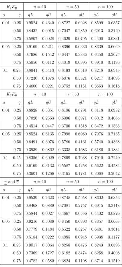
andK0. The resulting intervals [γ_i, γi] for three significance levels are given in Table

3.2. Note that we transformed the data using the overall values [γ, γ], derived as the minimum and maximum corresponding values for the pairwise tests, respectively.

In the second step of our method, we transformed the data using the [γ, γ] values. All observations at the increased stress levels were transformed to the normal stress level. Therefore, the observations at the increased stress levels K1 and K2 are transformed to interval-valued observations at the normal stress level K0. We

(42)

3.4. Examples 31 Case K0 = 283 K1 = 313 K2 = 353 K1 = 313 (×1.4) K2 = 353 (×0.4) 1 2692.596 241.853 74.557 338.595 29.823 2 3208.336 759.562 94.983 1063.387 37.993 3 3324.788 769.321 138.003 1077.050 55.201 4 5218.419 832.807 180.090 1165.930 72.036 5 5417.057 867.770 180.670 1214.878 72.279 6 5759.910 1066.956 187.721 1493.739 75.088 7 6973.130 1185.382 200.828 1659.535 80.331 8 7690.554 1189.763 211.913 1665.668 84.765 9 8189.063 1401.084 233.529 1961.517 93.412 10 9847.477 1445.231 298.036 2023.323 119.214

Table 3.1: Failure times at three temperature levels (first three columns) and changed failure times (last two columns), Example 3.4.1.

Significance level 0.01 0.05 0.10 Stress level γ i γi γi γi γi γi Case 1: K₁ K₀ 4060.018 6605.752 4424.881 6261.168 4593.700 6100.653 K2K0 4377.043 5602.321 4550.205 5434.908 4630.511 5357.037 Case 2: K₁×(1.4), K₀ 3066.539 5612.273 3431.402 5267.689 3600.221 5107.174 K2×(0.4), K0 5684.708 6909.985 5857.870 6742.573 5938.175 6664.701

(43)

3.4. Examples 32 0 5000 10000 15000 20000 25000 30000 260 280 300 320 340 t0 y0

Figure 3.1: Some transformed data using [4060.018,6605.752], Example 3.4.1. briefly illustrate this in Figure 3.1, using only three points of the data at each level, therefore, we have six lines going down from each level. We transformed the data from the higher stress levelsK1 andK2 using [γ, γ] = [4060.018,6605.752] with 0.01 level of significance, mixed with the original data at the normal stress level K0. Note that, in Figure 3.1 the two largest transformed data points are the γ and γ

transformations of the largest observation from level K2. So, this illustrates a key property of our method, that data transformed from higher levels tend to be wider intervals at the normal level.

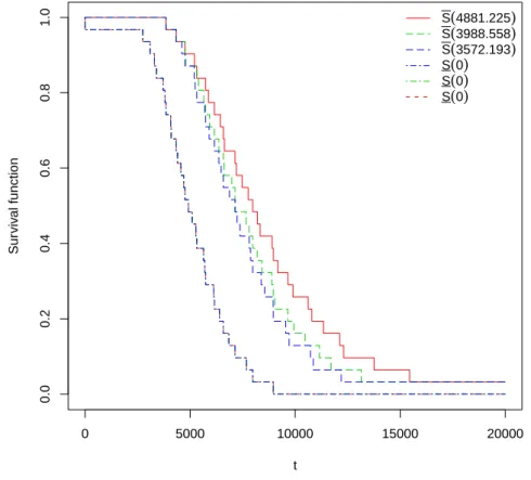
The NPI lower survival function is based on the original data at level 0 together with the transformed data from the stress levels K1 to K0 and K2 to K0 using γ. Similarly, the NPI upper survival function is based on the original data at level 0 together with the transformed data from the stress levels K1 to K0 and K2 to K0 using γ. The γ transformed the points to the smallest values and therefore is the most pessimistic case, which leads to the lower survival function S. The γ trans-formed the points to the largest values and therefore is the most optimistic case, which leads to the upper survival functionS. In Case 1, we have γ = 4060.018 and

γ = 6605.752, γ = 4424.881 andγ = 6261.168, andγ = 4593.700 andγ = 6100.653, which they are all equal to the values [γ, γ] that results from the pairwise test K1,

K0 with significance levels 0.01, 0.05 and 0.10, respectively. We used all the aboveγ andγ values to transform the data to the normal stress level 0, see Figure 3.2(a). In

Imprecise Statistical Methods for Accelerated Life Testing

Durham E-Theses

Imprecise Statistical Methods for Accelerated Life

Testing

Imprecise Statistical Methods for

Accelerated Life Testing

Abdullah Ali H. Ahmadini

A Thesis presented for the degree of

Doctor of Philosophy

Statistics and Probability

Department of Mathematical Sciences

University of Durham

England

April 2019

Dedicated to

Imprecise statistical methods for

accelerated life testing

Abdullah Ali H. Ahmadini

Submitted for the degree of Doctor of Philosophy

April 2019

Abstract

Declaration

Acknowledgements

Contents

Chapter 1

Introduction

1.1

Motivation

1.2

Outline of the thesis

Chapter 2

Background

2.1

Reliability testing

2.2

Accelerated life testing

2.3

Basic Statistical Methods

2.3.1

Likelihood ratio test

2.3.2

Log-rank test

2.4

Nonparametric predictive inference

Chapter 3

Statistical inference based on the

likelihood ratio test

3.1

Introduction

3.2

The model

3.3

ALT inference using likelihood ratio tests

3.4

Examples