Effects of highway geometric elements on accident modelling

(1)

EFFECTS OF HIGHWAY GEOMETRIC ELEMENTS

ON ACCIDENT MODELLING

MOHITA MOHAN GARNAIK

Department of Civil Engineering

National Institute of Technology Rourkela

Odisha -769 008, India

(2)

EFFECTS OF HIGHWAY GEOMETRIC ELEMENTS

ON ACCIDENT MODELLING

A THESIS SUBMITTED IN PARTIAL FULFILLMENT OF

THE REQUIREMENTS FOR THE DEGREE OF

MASTER OF TECHNOLOGY (RESEARCH)

IN

TRANSPORTATION ENGINEERING

BY

MOHITA MOHAN GARNAIK

ROLL NO. : 611 CE 305

Under the Guidance of

Dr. Ujjal Chattaraj

Department of Civil Engineering

National Institute of Technology Rourkela

Odisha -769 008, India

January 2014

(3)

Department of Civil Engineering National Institute of Technology Rourkela

Odisha -769 008, India

CERTIFICATE

This is to certify that the thesis entitled, “EFFECTS OF HIGHWAY GEOMETRIC

ELEMENTS ON ACCIDENT MODELLING” submitted by Mohita Mohan Garnaik

bearing roll no. 611CE305 in partial fulfilment of the requirements for the award of Master

of Technology (Research) degree in Civil Engineering with specialization in

“Transportation Engineering” during 2012-2014 session at the National Institute of

Technology, Rourkela is an authentic work carried out by him under my supervision and guidance.

To the best of my knowledge, the matter embodied in the thesis has not been submitted to any other University / Institute for the award of any Degree or Diploma.

January, 2014 Dr. Ujjal Chattaraj

Assistant Professor Department of Civil Engineering National Institute of Technology

(4)

ii

Acknowledgements

I take this opportunity to convey my deep sense of gratitude to my esteemed supervisor

Dr. Ujjal Chattaraj, for his invaluable guidance, keen interest and constant encouragement

rendered during entire course of the research work. In spite of his busy schedule, he participated in each and every minute details of my progress of work and shared both my pleasures and anxieties on the research findings. He was always available to me for technical discussion and clarification of doubts.

I express my sincere thanks to Prof. N. Roy (HOD) of Department of Civil Engineering, NIT, Rourkela, for providing me with all necessary administrative facilities during the research work.

I would also express my gratitude to Prof. M. Panda of Department of Civil Engineering, National Institute of Technology, Rourkela, for his guidance and the support in a lot of various aspects.

I am very much thankful to Prof. K. C. Biswal and Prof. H. B. Sahu of National Institute of Technology, Rourkela, for their valuable and timely advice for my research work.

I also convey my thanks to Mr. M. S. Rawat, Executive Director (Transportation) of M/s AECOM Asia Company Ltd. for providing necessary facilities to collect field data for conducting this piece of work.

I am also thankful to my all research friends for their friendship and companionship throughout my master programme.

I am thankful and express my gratitude to Highway Engineering Laboratory staff for their constant help, support and cooperation throughout the research work. I am very much thankful to all of them.

Last but not the least, I would like to express my gratitude to my parents and wife for their unwavering support and invariable source of motivation. Finally, I bow down before the Divine Providence who made everything possible.

(5)

iii

ABSTRACT

The tremendous traffic growth generally observed in road transportation has led to a lot of negative consequences in the form of road accidents both in developed and developing countries. This observation calls for considerable attention towards development a system for the road safety mechanism of rural highway. Road accident prediction plays an important role in accessing and improving the road safety. Fuzzy logic is one of the popular techniques in the broad field of artificial intelligence and ability to improve performance similar to human reasoning and describe complex systems in linguistic terms instead of numerical values. In this thesis, a system was established based on Fuzzy Inference System (FIS) in which output data such as traffic Accident Rate (AR) and input data such as various highway geometric elements. The study was conducted on two road segments from plain & rolling terrain highway and two road segments from mountainous & steep terrain highway within the rural area of the Indian Territory. Two Highway Accident Rate Prediction Models (HARPMPRT

and HARPMMST) were developed due to the complexity of geometric elements of rural

highway on different terrain conditions which take horizontal radius, superelevation, K-value, vertical gradient and visibility as input variables and Accident Rate (AR) as output variables. The findings show that the proposed model can be effectively applied as a useful Road Safety tool capable of identifying risk factors related to the characteristics of the road and great support to the decision making of incident management in Intelligent Transportation Systems. Significant positive relationships were also identified between the geometric elements and accident rate. A simulation study and real life data analysis are performed to demonstrate model fitting performances of the proposed model.

(6)

iv

List of Tables

Table 1.1: Terrain Classifications... 2

Table 3.1: Vehicles Classification System... 22

Table 3.2: Seasonal Correction Factor (SCF)... 23

Table 3.3: Summary of Annual Average Daily Traffic... 23

Table 4.1: Summary of Accident Rate of Highway... 31

Table 4.2a: Summary of Analysis of Variance of NH-200... 38

Table 4.2b: Summary of Analysis of Variance of NH-23... 38

Table 4.2c: Summary of Analysis of Variance of NH-87... 39

Table 4.2d: Summary of Analysis of Variance of NH-22... 39

Table 5.1a: Descriptive Statistics of the Calibration set of Data of NH-200... 56

Table 5.1b: Descriptive Statistics of the Calibration set of Data of NH-87... 56

Table 5.2a: Descriptive Statistics of the Validation set of Data of NH-23... 56

Table 5.2b: Descriptive Statistics of the Validation set of Data of NH-22... 56

Table 5.3a: Summary of Fuzzy Clustering of NH200 (HARPMPRT)... 58

Table 5.3b: Summary of Fuzzy Clustering of NH87 (HARPMMST)... 58

(11)

ix

List of Figures

Figure 1.1: Typical Horizontal Curve... 4

Figure 1.2: Typical Vertical Curve... 5

Figure 3.1a: Location Map of NH-22... 16

Figure 3.1b: Location Map of NH-87... 17

Figure 3.1c: Location Map of NH-23... 18

Figure 3.1d: Location Map of NH-200... 19

Figure 3.2: Topographic Points on Cross Sectional View... 21

Figure 3.3: Topographic Points on Plan View... 21

Figure 3.4: Typical Triangulation Integrated Network (TIN) of Existing Alignment... 24

Figure 3.5: Data Extraction on Horizontal Alignment... 25

Figure 3.6a: Sight Distance Achieved on Road Alignment... 27

Figure 3.6b: Sight Distance Not Achieved on Road Alignment... 28

Figure 4.1: Accident Rate versus Horizontal Radius... 32

Figure 4.2: Accident Rate versus Deflection Angle... 32

Figure 4.3: Accident Rate versus Horizontal Arc Length... 33

Figure 4.4: Accident Rate versus Superelevation... 34

Figure 4.5: Accident Rate versus Rate of Change of Superelevation... 34

Figure 4.6: Accident Rate versus Vertical Gradient... 35

Figure 4.7: Accident Rate versus Vertical Curve Length... 36

Figure 4.8: Accident Rate versus K-value ... 36

Figure 4.9: Accident Rate versus Visibility... 37

Figure 4.10a: Accident Rate on NH-200... 40

(12)

x

Figure 4.10c: Accident Rate on NH-87... 41

Figure 4.10d: Accident Rate on NH-22... 42

Figure 5.1: Representation of a crisp set... 44

Figure 5.2: Representation of a fuzzy set... 45

Figure 5.3: Representation of a S -function... 46

Figure 5.4: Representation of a -function... 47

Figure 5.5: Representation of a L -function... 47

Figure 5.6: Representation of a A -function... 48

Figure 5.7: Schematic diagram of a Fuzzy Inference System (FIS)... 51

Figure 5.8: Schematic Diagram of Proposed Model Structure... 54

Figure 5.9: Mamdani Type Fuzzy Inference System (MATLAB R2012b)... 55

Figure 5.10: Sample of Fuzzy Clustering... 57

Figure 5.11: Fuzzification of the Input Variable RA... 60

Figure 5.12: Fuzzification of the Input Variable SE... 62

Figure 5.13: Fuzzification of the Input Variable K... 63

Figure 5.14: Fuzzification of the Input Variable VB... 64

Figure 5.15: Fuzzification of the Input Variable RA... 66

Figure 5.16: Fuzzification of the Input Variable SE... 67

Figure 5.17: Fuzzification of the Input Variable G... 69

Figure 5.18: Fuzzification of the Input Variable VB... 70

Figure 5.19: Fuzzification of the Output Variable AR... 71

Figure 5.20a: Defuzzification of the Data Point of NH-200 (HARPMPRT)... 75

Figure 5.20b: Defuzzification of the Data Point of NH-87 (HARPMMST)... 76

Figure 5.21: Flow Chart of the Proposed Model... 77

(13)

xi

Figure 5.23: Results of Calibration Set Data of NH-87... 78

Figure 6.1: Simulated Accident Rate (AR) versus Accident Location of NH-23... 79

Figure 6.2: Simulated Accident Rate (AR) versus Accident Location of NH-22... 80

Figure 6.3a: Accident Rate (AR) versus Horizontal Radius... 81

Figure 6.3b: Accident Rate (AR) versus Superelevation... 81

Figure 6.3c: Accident Rate (AR) versus K-value... 82

Figure 6.3d: Accident Rate (AR) versus Visibility... 82

Figure 6.4a: Accident Rate (AR) versus Horizontal Radius... 83

Figure 6.4b: Accident Rate (AR) versus Superelevation... 83

Figure 6.4c: Accident Rate (AR) versus Vertical gradient... 83

(14)

xii

List of Appendices

Appendix-3.1: Traffic Volume Count on NH-22... 93

Appendix-3.4: Traffic Volume Count on NH200... 94

Appendix-4.1(a): Details of Horizontal Radius on NH-200 and NH-23... 95

Appendix-4.1(b): Details of Horizontal Radius on NH-87 and NH-22... 96

Appendix-4.2(a): Details of Deflection Angle on NH-200 and NH-23... 97

Appendix-4.2(b): Details of Deflection Angle on NH-87 and NH-22... 97

Appendix-4.3(a): Details of Horizontal Arc Length on NH-200 and NH-23... 98

Appendix-4.3(b): Details of Horizontal Arc Length on NH-87 and NH-22... 98

Appendix-4.4(a): Details of Superelevation on NH-200 and NH-23... 99

Appendix-4.4(b): Details of Superelevation on NH-87 and NH-22... 99

Appendix-4.5(a): Details of Rate of change of Superelevation on NH-200 and NH-23... 100

Appendix-4.5(b): Details of Rate of change of Superelevation on NH-87 and NH-22... 101

Appendix-4.6(a): Details of Vertical Gradient on NH-87 and NH-22... 102

Appendix-4.6(b): Details of Vertical Gradient on NH-87 and NH-22... 102

Appendix-4.7(a): Details of Vertical Curve Length on NH-200 and NH-23... 103

Appendix-4.7(b): Details of Vertical Curve Length on NH-87 and NH-22... 103

Appendix-4.8(a): Details of K-value on NH-200 and NH-23... 104

Appendix-4.8(b): Details of K-value on NH-87 and NH-22... 104

Appendix-4.9(a): Details of Visibility/Sight Distance on NH-200 and NH-23... 105

Appendix-4.9(b): Details of Visibility/Sight Distance on NH-87 and NH-22... 105

(15)

xiii

Abbreviations and Notations

AADT Average Annual Daily Traffic ANOVA Analysis of Variances

AR Accident Rate

CoG Center of Gravity

FIS Fuzzy Inference System

F F-test (F statistical hypothesis)

ITS Intelligent Transportation Systems

NH National Highway

R2 Correlation Coefficient SCF Seasonal Correction Factor

MS Mean of Square

SS Sum of Square

VCL Vertical Curve Length

A A notation of set

U A notation of set

x Element of set

X Universal set

y Output for fuzzy inference system Parameter of fuzzy set

Parameter of fuzzy set Parameter of fuzzy set

(16)

1

Chapter 1 Introduction

1.1 Background

Motor vehicle accidents kill about 1.2 million people a year world-wide and the number will grow to more than 2 million in 2020 unless steps are taken, a study released by the World Health Organisation (WHO) and the World Bank has found [Washington: Article-Traffic accidents becoming one of world's great killers, By Matthew Wald, April 8, 2004]. WHO has revealed in its first Global Status Report on Road Safety that more people die in India due to road accidents than anywhere else in the world, including the more populous China [New Delhi:Articles.timesofindia.indiatimes.com/2009-08-17].

Road transport plays vital role in economic development, trade and social integration, which rely on the conveyance of both people and goods. Vehicular traffic carrying goods and people increases with the increasing economy resulting in an increase of traffic accidents. Three major factors causing traffic accidents are human, road and vehicles. The human factor has the most significant effect on accident. However, this factor is governed by an individual thought process and cannot be studied empirically. Moreover, any design solution mitigating this kind of individual human behaviour cannot be predicted only some safety rules can be enforced. Also, different mechanical behaviour of vehicles factors are not the scope of civil engineering study. Hence, road factors are only considered as a part of this study. It is very important for the highway to establish a harmony between the all the three factors at the

(17)

2

design stage of a highway. With a geometrically good design, it is possible to compensate for the other factors and thus decrease the number of traffic accidents (A.F. Iyinam et al., 1997).

1.2 Objectives

The high socio-economic cost of the injuries and fatalities, occurring due to road accidents and the need for effective policies for curbing road accidents make it imperative to study the causes of road accidents. The present study aims to detect and identify the role of alignment geometric elements on accident and prediction of accident rate through artificial intelligence system modelling.

1.3 Basic Parameters of Highway Geometric

1.3.1 Terrain/Topography

The classification of the terrain is done by means of cross slope of the country, i.e., slope approximately perpendicular to the center line of the highway location. To characterize variations in topography, engineers separate it into four classifications according to terrain as listed in Table 1.1.

Table 1.1: Terrain Classifications

Terrain Classification Cross slope of country (%)

Plain Less than 10

Rolling Greater than 10 up to 25

Mountainous Greater than 25 up to 60

(18)

3

1.3.2 Speed

Speed is defined as the distance covered per unit time. Since speed of every vehicle is impossible to track on a roadway; therefore, in practice, average speed is based on the sampling of vehicles over a period of time on a particular section of road. Speed is one of the most important factors considered by travellers in selecting alternative routes. The speed of a vehicle on a road depends upon five conditions: physical characteristics of the highway, amount of roadside interference, weather, presence of other vehicles, and the speed limitations in addition to the capabilities of the driver and their vehicles. It is the basic parameter which determines all other geometric features of the highway.

1.3.3 Horizontal Alignment

The horizontal alignment is the route of the highway, defined as a series of horizontal tangents and curves. Horizontal curve is the curve in plan to change the direction of the center line of the highway. The geometries of horizontal alignment are based on an appropriate relationship between design speed and curvature and on their joint relationship with superelevation and side friction. Typical horizontal curve furnished in figure 1.1as per Indian Road Congress (IRC) guidelines (IRC: 38-1988 & IRC: 73-1980).

(19)

4

Figure 1.1: Typical Horizontal Curve

Where

: Total deflection angle L : Total length of curve

IP : Intersection point of tangents ST : Short tangent

RC : Radius of circular curve LT : Long tangent

LS : Length of spiral curve Ts : Total tangent distance

LC : Length of circular curve Es : External distance

1.3.4 Vertical Alignment

Vertical alignment is the longitudinal section of a roadway to provide easy and safe change of gradient. It is defined as a series of gradients and vertical curves. Gradient is the rate of rise or fall with respect to the horizontal along the length of a road expressed as a percentage or as

(20)

5

a ratio or in degrees. Vertical curves to effect gradual changes between gradients with any one of the crest or sag types and result is safe and comfortable in operation, pleasing in appearance, and adequate for drainage. The typical vertical curve in crest condition is furnished in figure 1.2 as per IRC: 23-1989.

Figure 1.2: Typical Vertical Curve

Where

VIP : Vertical point of intersection. g : Gradient

MO : Mid-ordinate

g : Algebraic difference in grades (percent) of the grades tangents. VCL : Vertical curve length measured horizontally.

BVC : Beginning of vertical curve EVC : End of vertical curve

(21)

6

1.3.5 Cross Section

Cross section is defined as the number of lanes and lane width including cross fall, shoulder, sidewalk, earth slope and drainage features in the transverse direction of the roadway. The cross section shows the total formation of the road.

1.3.6 Superelevation

Superelevation is tilting or banking the roadway to counteract the centripetal force developed as the vehicle moves around the horizontal curve. When a vehicle moves in circular path, it undergoes a centripetal acceleration that acts towards the centre of curvature. This acceleration is sustained by a component of the vehicle’s weight related to the roadway superelevation, by the side friction developed between the vehicle’s tires and or the pavement surface.

1.3.7 Sight Distance

Sight distance is the distance along the road surface at which a driver has visibility of object at a specified height above the carriageway. This is the adequate length along the highway in the different situations to permit drivers enough time and distance to control their vehicles so as to avoid unforeseen accidents.

1.3.8 Traffic Volume

1.3.8.1 Average Daily Traffic (ADT)

Traffic volume is defined as total traffic movement on the highway in both directions at a particular point in terms of average daily traffic (ADT) volume. The ADT is defined as the total volume during a given period, greater than one day and less than one year, divided by the number of days in that time period.

(22)

7

1.3.8.2 Annual Average Daily Traffic (AADT)

Annual Average Daily Traffic (AADT) is defined as the total traffic volume passing a point or segment of a highway facility in both directions for one year divided by the number of days in the year. It is one of the important traffic variables required for analysis of traffic crash rates.

AADT is calculated by incorporating the seasonal variations in traffic movement on the study road. Seasonality aspect can be captured through direct variables such as month-wise classified traffic count data for past one or two years at different road locations. Other methods involve identifying surrogate variables such as monthly sales of petroleum products, monthly tourist data, monthly traffic record at check-posts, etc.

1.4 Accident Statistics

1.4.1 Cost of Road Accident

Road accidents carry high economic and social costs, which are not easy to measure. The cost of road related injuries and accidents can be viewed in terms of (a) medical costs (b) other cost related to administrative legal and police expenditure (c) collateral damage in terms of damage to property and motor vehicle and (d) loss due to income. In addition, accident survivors often live a poor quality of life and have to live with pain and suffering which are difficult to estimate. In economic terms, the cost of road crash injuries creates direct impact to gross domestic product (GDP) of the country.

1.4.2 Profile of Road Accident

The total numbers of accidents reported by all the States/ Union Territories (UTs) in the year 2012 were 4.90 lakhs of which 1.38 lakh people were killed and more than 5 lakh persons

(23)

8

injured, many of whom are disabled for rest of their lives (Source: Ministry of Road Transport & Highways). These numbers translate into one road accident every minute, and one road accident death in less than four minutes. Occurrence of accidents is an outcome of factors which include type of road users, colliding vehicles, environmental/road related factors (road geometry, design, visibility etc), vehicle related, nature of traffic management, composition and flow of road traffic and adherence/enforcement of road safety regulations. The main thrust of accident prevention and control across the world has been on Education, Enforcement, Engineering and Environment & Emergency care of accident victims.

1.4.3 Spatial Distribution of Road Accidents (Urban vis-à-vis Rural)

In 2012, the total number of accidents that occurred in rural areas was at 54.3 per cent while the rest occurred in urban areas. The number of persons injured in rural areas was also higher at 60.2 per cent as compared to urban areas.

1.4.4 Time of Occurrence of Road Accidents

For framing strategies for prevention and organization of care of accident victims, information on timing of accidents is a prerequisite. During 2012, high rates of road accidents were observed between 3pm–6pm, 9am–12am and 6pm–9pm. The distribution of the total accidents during night time (6pm to 6am) and day time (6am to 6pm) is approximately in the ratio of 2:3 i.e. about 40 per cent during night time and 60 per cent during daytime.

Motor vehicle population has recorded significant growth over the year. The motor vehicle growth is higher than the rate of road network developed in India. Different elements of highway geometric as well as surface condition of highway have great influence in occurrence of traffic accidents. To minimize traffic accidents, great attention has to be paid in

(24)

9

achieving consistency in highway design, minimize the frequency and extent of violations of driver expectancy and emphasis on concerns of three-dimensional (3D) highway design to achieve a “safe-by-design” (George Kanellaidis et al.,2011).

The current chapter, contains the motivation, aim and scope of the study and the main hypothesis of the study as an introduction.

In next chapter, traffic accident prediction models in the literature were examined, and it was recognized that numbers of researcher widely used Linear and Negative Binomial Models. As a result, the use of fuzzy logic method was decided to establish accident rate prediction model.

(25)

10

Chapter 2 Literature Review

The study is an effective traffic accident modelling in minimizing the accident rates depending on road factors and finding the impact of highway geometric elements. Hence, a literature survey was carried out in the field of accident causative factors and accident prediction and optimisation modelling and presented as below.

2.1 Accident Causative Factors Overview

Feng-Bor Lin (1990) studied on flattening of horizontal curve on rural two lane highways and found that horizontal curves on highways are on average more hazardous than tangent sections. As their curvatures increase, horizontal curves tend to have higher accident rates. He suggests that the differences between the 85th percentile speeds and the safe speeds have no statistically significant relationships with the accident rates. In contrast, the magnitudes of speed reduction, when vehicle moves from a tangent section to a curve, have a significant impact on traffic safety. Such speed reductions on horizontal curve with gentle grades are strongly correlated with the curvatures of the curves. Therefore, curvatures can be used as a safety indicator of the curves.

Y. Hassan et al. (2003) studied on effect of vertical alignment on driver perception of horizontal curves and found that perception of the driver of the road features ahead is an important human factor and should be addressed in road design. An erroneous perception of the road can lead to actions that may compromise traffic safety and poor coordination of horizontal and vertical alignments is believed to cause such wrong perceptions. Through

(26)

11

statistical analysis, they suggested that the horizontal curvature looked consistently sharper when it overlapped with a crest curve and consistently flatter when it overlaps with a sag curve.

Zhang Yingxue (2009) analysed the relation between highway horizontal curve and traffic safety and found that curve radius, super-elevation, widening, transition curve and sight distance have the important effect on traffic accidents,

Ali Aram (2010) studied on effective safety factors on horizontal curves of two-lane highway and observed that several traffic volumes and mix, geometric features of the curve, cross section, roadside hazards, stopping sight distance, curve coordination, pavement friction and traffic control devices affect the safety performance of horizontal curve. He found that degree of horizontal curve, length of curve, superelevation, transition length, shoulder width and ADT responses are the important independent effective variables. He also suggested that horizontal curves have higher crash rates than straight section of similar length and traffic composition.

Kay Fitzpatrick et al. (2010) studied on horizontal curve accident modification factor with consideration of driveway density on rural four-lane highways in Texas. They developed horizontal curve accident modification factor (AMF) for rural four-lane divided and undivided highways and determined the effect of driveway density is different for horizontal curves as compared to tangent sections. Negative binomial regression models were used to determine the effects of independent variables on crashes.

George Kanellaidis et al. (2011) studied highway geometric design from the perspective of recent safety developments and suggested emphasis on concerns of three-dimensional (3D) highway design to achieve a “safe-by-design”.

(27)

12

2.2 Accident Prediction Model

Eric T. Donnell et al. (2009) studied on appraisal of the interactive highway safety design model’s crash prediction and design consistency modules and evaluated the safety and operational effects of geometric on two lane rural highways through interactive highway safety design model (IHSDM). The design consistency module can evaluate the alignment complexity and thus predict the accident.

Jaisung Choi et al. (2011) studied on the safety effects of highway terrain types in a crash model and suggested that when the design speed is changed, the terrain types will have some safety effects using regression analysis. The statistical analysis was performed with an ordinal logistic regression model in order to relate several independent variables of highway geometric elements such as terrain type, tangent length, curve length, radius of curvature and vertical grade to actual crash occurrences. Through this investigation, terrain type was found to be a significant independent variable that explains crash occurrences for rural arterial roads in South Korea.

O. F. Cansiz et al. (2011) studied artificial neural network to predict collisions on horizontal tangents of 3D two-lane highways and explored the safety effects of horizontal tangents combined with vertical curves using artificial neural network (ANN) models. The collision prediction models were established using artificial neural network for these horizontal tangents and were compared with the existing regression models. The ANN method provided better results for predicting collision frequency on horizontal tangents. They identified the variables which are related to vertical curves, horizontal tangents, and cross-sections. The regression models were estimated using the significant variables for all combinations.

(28)

13

Fajaruddin Mustakim et al. (2011) were developed accident predictive models for rural roadway in Malaysia using multiple non-linear regression method with the road and traffic flow explanatory variable and concluded that, the existing number of major access points, without traffic light, rise in speed, increasing number of Annual Average Daily Traffic (AADT), growing number of motorcycle and motorcar and reducing the time gap are the potential contributors of increment accident rates on multiple rural roadway.

Iljoon Chang et al. (2012) were developed model for identifying accident-prone spots based on the total number of accidents. They considered a mixture of the zero-inflated Poisson and the Poisson regression models to analyze zero-inflated data sets drawn from traffic accident studies.

Miloud Driss et al. (2013) studied on traffic accident prediction system based on fuzzy logic which allows to identify “the degree of exposure to road accidents’ risk”, and to analyze the level of complexity of the factors involved. A Geographic Information System (GIS) was integrated into the analysis process to enable a spatial visualization of the degrees of exposure to road accidents’ risk, provided a cartographically measurable solution to establish and attenuate accident risk. The developed system can be effectively applied to identifying risk factors related to the characteristics of the road.

2.3 Accident Optimisation Model

A.F. Iyinam et al. (1997) studied relationship between highway safety and road geometric design elements and observed that the relationship between safety and road geometric has meaningful relationships through regression analysis. They suggested that the control of the road factor is much easier than the human factor and by making a geometrically good design, it was even possible to compensate for the other factors and thus decrease the number of

(29)

14

traffic accidents through a regression analysis is made between the geometric parameters and accident rates.

2.4 Summary of the Literature Review

Highway geometric elements have great influence in traffic accidents and also effective factors on highway safety. As the relationships between highway accidents and highway geometric elements are considered some relationships are seen intuitively at a first approach. However, the important point is to determine the intensity of these relationships quantitatively.

Apart from the above study, many researchers recommended other promising methodologies like artificial neural networks, fuzzy methods and genetic algorithms for development of crash model.

(30)

15

Chapter 3 Empirical Data Collection and Extraction

3.1 Background

For this study, two roads in plain & rolling terrain National Highway (NH) 23 &200 and two roads in mountainous & steep terrain National Highway 22 & 87 were selected. Various field data such as 3D Topographic features, Accident records and Traffic volume were collected for these roads. Careful observation and collection of such data with accuracy were carried out.

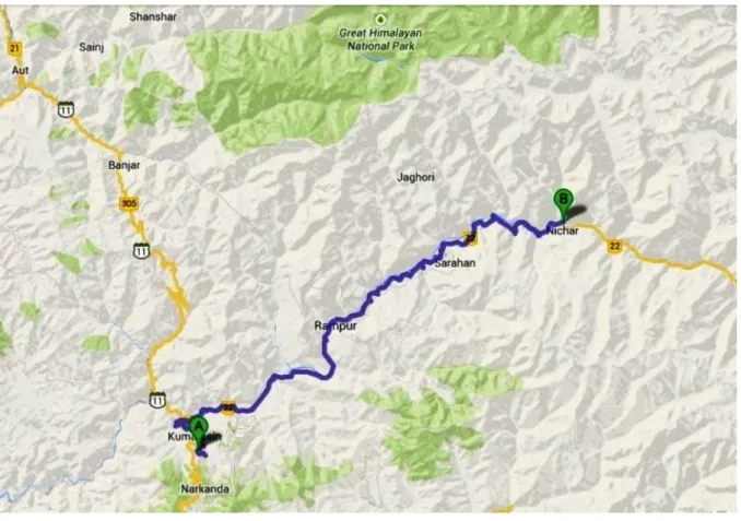
National Highway 22 (NH-22) is a 459 km National Highway in Northern India that runs from Ambala through Chandigarh and Himachal Pradesh up to Khab on the Chinese border. The study corridor takes off from km 230/0 near village Narkanda, traverse in south-northeast direction and end at km 330/0 near village Wangtu. This part of the road falls in the state of Himachal Pradesh and situated between 31 18.78' N & 31 44.48' N latitude, 77 27.28' E & 78 44.14' E longitude. Total length of the study corridor is about 100km and study area is given under Figure 3.1a.

(31)

16

Figure 3.1a: Location Map of NH-22

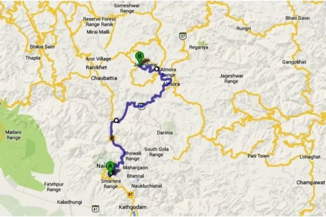
National Highway 87 (NH-87) is a National Highway in Northern India. NH-87, which runs for a distance of 316 km, links Rampur in Uttar Pradesh with Karna Prayag in Uttarakhand. The study corridor takes off from km 10/0 at village Jeolikote, traverse in south-north direction and end at km 80/0 near village Kharkuna. This part of the road falls in the state of Uttarakhand and situated between 29 20.65' N & 29° 38.33' N latitude, 79° 28.98' E & 79° 34.56' E longitude. Total length of the study corridor is about 70km and the study area is given under Figure 3.1b.

(32)

17

Figure 3.1b: Location Map of NH-87

National Highway 23 (NH-23) is a 459 km National Highway in central-eastern India that connects Chas in Jharkhand with the intersection of National Highway 42 at Banarpal in Odisha. The study corridor takes off from km 338/0 at village Pallahara, traverse in north- south direction and end at km 405/0 near Talcher. This part of the road falls in the state of Odisha and situated between 21° 25.92' N & 20° 56.84' N latitude, 85° 11.21'E & 85° 16.30'E longitude. Total length of the study corridor is about 67km and study area is given under Figure 3.1c.

(33)

18

Figure 3.1c: Location Map of NH-23

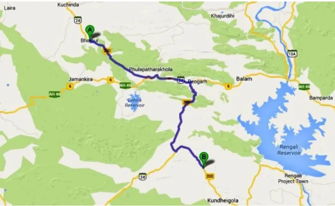
National Highway 200 (NH-200) is a 740 km National Highway in central-eastern India that connects Raipur, the state capital of Chhattisgarh to Chandikhole in Odisha. The study corridor takes off from 130/0 at village Bhojpur, traverse in north-south direction and end at km 190/0 near village Chhatabar. This part of the road falls in the state of Odisha and situated between 21° 25.92' N & 20° 56.84' N latitude, 85° 11.21' E & 85° 16.30' E longitude. Total length of the study corridor is about 60km and the study area is given under Figure 3.1d.

(34)

19

Figure 3.1d: Location Map of NH-200

3.2 Data Collection

3.2.1 Topographic Survey

The topographic survey has been carried out with Total Station survey equipment at accident locations. Total Station is a high precision surveying equipment to carry out 3-dimensional feature of the existing road. This survey equipment can measure distance, angle, and co-ordinates with relative to the known position and it calculates using coordinate geometry and triangulation. All the measurements are controlled by an internal programme & interfaced via computer. The captured digital data has been downloaded into a CAD programme (AutoCAD) to visualize the surveying data as vector entities. Finally, this data has been analysed later with the design application software (MX Road) which is extensively used for highway design.

(35)

20

3.2.1.1 Topographic Survey Methodology

In order to have the accurate topographical survey work, a network of horizontal control has been established using differential GPS techniques and levelling network using Digital Auto Levels. The fixing of major control stations, the station points are embedded in the ground, in pair with inter visibility with a distance of around 200m. The horizontal control coordinates were observed and worked out by use of GPS instrument for each pair and the elevation were provided by an independent levelling survey by Digital Auto Level. These Major Control Stations were kept at a distance of 500m at a safe location.

The control traverse is the base framework for all the further survey work. This provides a coordinated horizontal grid and a level reference system to ensure accuracy. Thus the measured coordinates of these survey grids (Northing and Easting) and the levels are to be tied to GTS benchmark wherever available, to verify the accuracy of survey. The GPS/ Benchmark points and Reference Benchmark points established acted as both horizontal and vertical control points.

Levels along centre line of the existing road are taken at every 10m interval and at all intermediate breaks in ground using Total Station. The said spacing has suitably reduced at horizontal curves to 5m. Cross sections are taken at every 20 m intervals and at each cross section the survey normally extends beyond 20m on each side of the existing road center line with survey points at 5-10 m apart and at all variations in the natural ground or breaks in level. The topographic survey thus carried out contains the details of all physical and topographical features within the survey corridor. The survey data were processed and converted to graphic files using Highway Design software called “MX Road”.

(36)

21

The 3D topographic points have been carried out along the road as given under Figure 3.2 and Figure 3.3.

Figure 3.2: Topographic Points on Cross Sectional View

Figure 3.3: Topographic Points on Plan View

3.2.2 Accident Record

Accident records have been collected from concerned police station from their accident record books. All these accident points have been verified with policemen as well as local villagers at the site.

3.2.3 Traffic Volume

The primary objectives of traffic surveys are to determine the characteristics of traffic movement in the study corridor. To find out the annual average daily traffic (AADT), three

(37)

22

days traffic survey has been carried out at the respective location of the road. Also, the traffic volume has been collected from concerned department (Public Works Department) and verified with three day traffic survey to compare with the existing data.

3.2.3.1 Traffic Survey Methodology

The homogeneous traffic sections have been identified based on the locations of major intersection along the study corridor. The directional classified traffic volume count has been carried out for each traffic homogeneous section for 24 hours a day continuously for 3 days. The survey stations have been located, away from urban area and villages to minimize interference of local traffic. The traffic count data analysis would present realistic forecast of traffic volume. Classified manual traffic counts have been recorded in 15 minutes intervals, using Tally marks on a standard format. The vehicle classification has been prepared as per IRC: SP 19-1991 and IRC: 9-1972 code requirements as given in Table 3.1.

Table 3.1: Vehicles Classification System

Motorized Vehicle Non Motorised Vehicle

2-Wheeler & 3-Wheeler Cycle

Passenger Car Cycle Rickshaw

Utility Vehicle (Jeep, Van, etc.) Animal Drawn Vehicle Bus (mini bus, standard bus) Other Non-Motorized Vehicle

Light Commercial Vehicle (freight) Truck

MCV (2-axle rigid chassis) HCV (Multi-axle Rigid) HCV (Multi-axle articulated)

Agricultural Tractors (with trailer/without trailer)

The purpose of the survey was to calculate the Average Daily Traffic (ADT) on the traffic homogeneous sections and to convert the traffic into Annual Average Daily Traffic (AADT)

(38)

23

with the multiplication of seasonal correction factor. The seasonal correction factors (SCF) adopted for the calculation of AADT has been furnished in Table 3.2.

Table 3.2: Seasonal Correction Factor (SCF)

Sl. No. Study Corridor Seasonal Correction Factors (SCF)

1 NH-22 0.96

2 NH-23 1.15

3 NH-87 0.85

4 NH-200 1.10

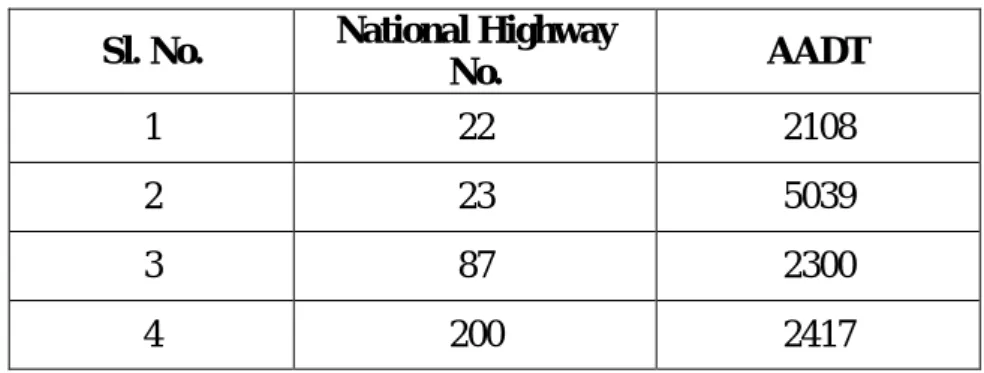
The summary of daily traffic count present in Appendix-3.1 to Appendix-3.4 and AADT in all study corridors have been furnished in Table 3.3.

Table 3.3: Summary of Annual Average Daily Traffic

Sl. No. National Highway

No. AADT 1 22 2108 2 23 5039 3 87 2300 4 200 2417 3.3 Data Extraction

To find out the geometric parameters of the existing road, topographic survey points (X, Y and Z / Easting, Northing and Elevation), road center line, carriageway edge and shoulder edge line has been imported to MX Road software and a 3-dimensional digital terrain model (DTM) was developed. Then Triangulation Integrated Network (TIN) was modelled as 3-dimensional surface. After this, geometric elements such as horizontal curve radius and Horizontal curve length, deflection angle, superelevation / crossfall, vertical gradient, vertical

(39)

24

curve length and sight distance have been extracted. The Triangulation Integrated Network (3D Model) developed along the road is given under Figure 3.4.

Figure 3.4: Typical Triangulation Integrated Network (TIN) of Existing Alignment

3.3.1 Data Extraction Methodology

The geometric elements of existing road at accident locations have been extracted as described under sub sections.

3.3.1.1 Horizontal Radius

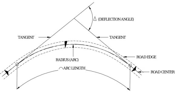
The existing radius has been measured from the best fitted radius with the existing road alignment. In this process, the two tangents are fixed with the existing center line and then, radius fitted with the two tangents, which is the best fit with existing alignment. The unit of the radius is metre. Horizontal parameters extracted from existing alignment on an accident location have been furnished in Figure 3.5 (using AutoCAD) as expressive sample.

Hilly Side

Valley Side Road

(40)

25 TANGENT (DEFLECTION ANGLE) RADIUS (ARC) TANGENT ARC LENGTH ROAD EDGE ROAD CENTER

Figure 3.5: Data Extraction on Horizontal Alignment

3.3.1.2 Deflection Angle

The tangents have been fixed on the existing road alignment on curve approaches. The total angle between the two tangents is called deflection angle and measured the same. The unit of the deflection angle is degree-minutes-seconds (DMS) or decimal degree.

3.3.1.3 Horizontal Arc Length

The arc length has been measured from the best fit radius with the two tangents in existing road alignment. The unit of the arc length is metre.

3.3.1.4 Superelevation / Cross Fall

The cross section of the existing road alignment has been developed from Digital Terrain Model (DTM) in every 10m interval through software on accident location. The maximum superelevation has been considered on outer side edge of carriageway in the horizontal curvature section. The unit of the superelevation is %.

(41)

26

3.3.1.5 Rate of change of Superelevation

The cross section of the existing road alignment has been developed from Digital Terrain Model (DTM) in every 10m interval through software on accident location. The rate of change of superelevation is calculated from the average of the rate of change of cross fall of consecutive cross section in the superelevation runoff section. The unit of the rate of change of superelevation is 1in n meter.

3.3.1.6 Vertical Gradient

From the digital terrain model, the longitudinal section of the existing road center line has been developed with the software, and then, the maximum vertical gradient measured from the existing longitudinal section / profile of the road on accident location.

3.3.1.7 Vertical Curve Length

From the digital terrain model, the longitudinal section of the existing road center line has been developed with the software and then the vertical gradient was fitted on existing longitudinal section on grade part and then the best fitted parabolic curve was fixed in between two grades. The best fitted vertical curve length has been measured. The unit of the vertical curve length is metre.

3.3.1.8 K-value of Vertical Curve (K)

The K-value or equivalent radius of vertical curve defines the sharpness or flatness of the vertical curve. This is a ratio of parabolic curve length and change of vertical grade. Also, this is horizontal distance required to effect a one percent change in gradient. This is

expressed as:

g VCL

(42)

27

3.3.1.9 Visibility /Sight Distance

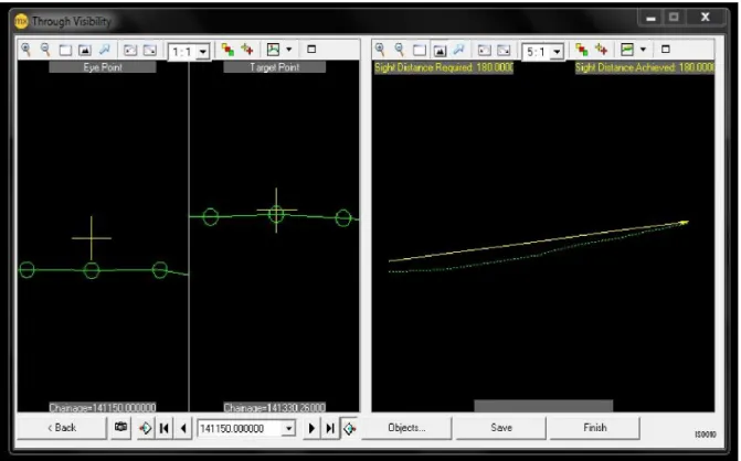
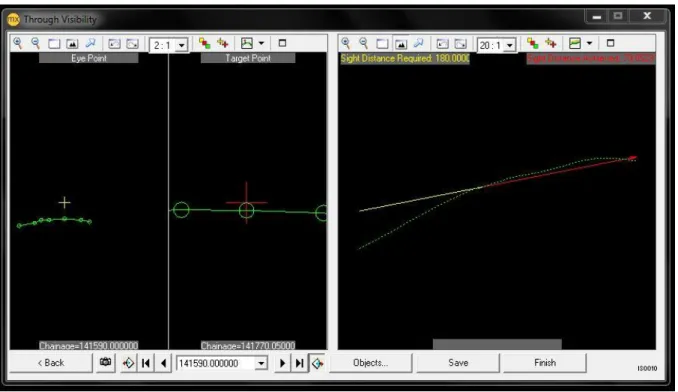
Sight distance has been measured with function of the horizontal and vertical alignment, in a 3D coordinate system. The actual sight distance has been generated along the road alignment through software considering with eye height and object height as 1.2m and 0.15m respectively. The achieved sight distancehas been calculated in every 10m interval and the minimum sight distance is considered at the accident location. The figure 3.6 shows an example of measurement of sight distance along the existing roadway.

(43)

28

Figure 3.6b: Sight Distance Not Achieved on Road Alignment

3.4 Summary

Total 339 numbers of accident locations have been considered on the 297km segment of road length in the plain & rolling and mountainous & steep terrain in rural areas. Data collected include: accident counts, traffic volume count (Average Daily Traffic), 3-D topographic survey of horizontal and vertical alignments.

The details of geometric elements of highway have been extracted through software with high accuracy level. These geometric elements are horizontal radius, deflection angle, horizontal arc length, superelevation, rate of change of superelevation, vertical gradient, vertical curve length, K-value and visibility/sight distance.

The collected data provide a comparatively varied and comprehensive basis for analysis and modeling. Driver and vehicle characteristics were neither collected, nor considered for

(44)

29

accident modeling. The highway geometric parameters have been analysed with accident rate in the next chapter.

(45)

30

Chapter 4 Analysis of Empirical Data and Results

4.1 Background

Accident analysis has been carried out in order to determine the effects of different geometric elements of the highway with accident rate of the same highway. These geometric elements are horizontal radius, deflection angle, horizontal arc length, superelevation, rate of change of superelevation, vertical gradient, vertical curve length, K-value and visibility/sight distance. Finally, these geometric elements are statistically analysed and considered for model development which are statistically significant.

4.2 Accident Rate

The accident rate is defined as the ratio between the number of accidents which happened in a given year and the number of vehicles with kilometres of travels length during that same year. It is generally expressed in crashes per million vehicle-kilometres of travel.

L N V C AR 365 000 , 000 , 100

The variables in this equation are:

AR = Accident Rate expressed as crashes per 100 million vehicle-kms of travel (100mvkm) C = Total number of crashes in the study period

V = Traffic volumes using Annual Average Daily Traffic (AADT) N = Number of years of data

(46)

31

The summary of Accident Rate in all study corridors have been furnished in Table 4.1. Table 4.1: Summary of Accident Rate of Highway

Variables NH-22 NH-23 NH-87 NH-200 C 58 165 62 54 V 2108 5039 2300 2417 N 3 3 3 3 L 100 66.5 70 60 AR 25.13 44.97 35.17 34.01

4.3 Analysis of Geometric Variables

The existing geometric elements of highway has been analysed with accident rate of the same highway. Also, the variables are grouped with same manner as per highway terrain condition.

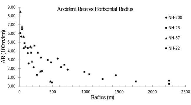
4.3.1 Analysis of Accident Rate versus Horizontal Radius

Total number of accidents has been counted within appropriate range of radius and then, the accident rate has been calculated as illustrated in Appendix-4.1and same has been plotted in Figure 4.1.

(47)

32

Figure 4.1: Accident Rate versus Horizontal Radius

4.3.2 Analysis of Accident Rate versus Deflection Angle

Total number of accidents has been counted in every 100 interval of deflection angle and then, the accident rate has been calculated as illustrated in Appendix-4.2 and same has been plotted in Figure 4.2.

Figure 4.2: Accident Rate versus Deflection Angle

0.00 1.00 2.00 3.00 4.00 5.00 6.00 7.00 8.00 9.00 0 500 1000 1500 2000 2500 A R ( 1 0 0 m v k m ) Radius (m)

Accident Rate vs Horizontal Radius

NH-200 NH-23 NH-87 NH-22 0.00 1.00 2.00 3.00 4.00 5.00 6.00 7.00 8.00 9.00 10.00 0 50 100 150 200 A R ( 1 0 0 m v k m )

Deflection Angle (Degree) Accident Rate vs Deflection Angle

NH-200 NH-23 NH-87 NH-22

(48)

33

4.3.3 Analysis of Accident Rate versus Horizontal Arc Length

Total number of accidents has been counted within appropriate range of arc length and then, the accident rate has been calculated as illustrated in Appendix-4.3and same has been plotted in Figure 4.3.

Figure 4.3: Accident Rate versus Horizontal Arc Length

4.3.4 Analysis of Accident Rate versus Superelevation

Total number of accidents has been counted in every 1% interval of superelevation and then, the accident rate has been calculated as illustrated in Appendix-4.4 and same has been plotted in Figure 4.4. 0.00 2.00 4.00 6.00 8.00 10.00 12.00 14.00 0 100 200 300 400 500 600 A R ( 1 0 0 m v k m ) Arc Length(m) Accident Rate vs Arc Length

NH-200 NH-23 NH-87 NH-22

(49)

34

Figure 4.4: Accident Rate versus Superelevation

4.3.5 Analysis of Accident Rate versus Rate of change of Superelevation

Total number of accidents has been counted within appropriate range of rate of change of superelevation and then, the accident rate has been calculated as illustrated in Appendix-4.5and same has been plotted in Figure 4.5.

Figure 4.5: Accident Rate versus Rate of Change of Superelevation

0.00 2.00 4.00 6.00 8.00 10.00 12.00 14.00 16.00 18.00 20.00 0 2 4 6 8 10 12 A R ( 1 0 0 m v k m ) Superelevation (%) Accident Rate vs Superelevation

NH-200 NH-23 NH-87 NH-22 0.00 2.00 4.00 6.00 8.00 10.00 12.00 14.00 16.00 18.00 0 200 400 600 800 1000 A R ( 1 0 0 m v k m )

Rate of change of Superelevation (1 in n) Accident Rate vs Rate of change of Superelevation

NH-200 NH-23 NH-87 NH-22

(50)

35

4.3.6 Analysis of Accident Rate versus Vertical Gradient

Total number of accidents has been counted in every 1% interval of vertical gradient and then, the accident rate has been calculated as illustrated in Appendix-4.6 and same has been plotted in Figure 4.6.

Figure 4.6: Accident Rate versus Vertical Gradient

4.3.7 Analysis of Accident Rate versus Vertical Curve Length

Total number of accidents has been counted in every 25m interval of vertical curve length and then, the accident rate has been calculated as illustrated in Appendix-4.7 and same has been plotted in Figure 4.7.

0.00 2.00 4.00 6.00 8.00 10.00 12.00 14.00 0 2 4 6 8 10 A R ( 1 0 0 m v k m ) Vertical Gradient (%) Accident Rate vs Vertical Gradient

NH-200 NH-23 NH-87 NH-22

(51)

36

Figure 4.7: Accident Rate versus Vertical Curve Length

4.3.8 Analysis of Accident Rate versus K-value

Total number of accidents has been counted in every 25m interval of vertical curve length and then, the accident rate has been calculated as illustrated in Appendix-4.8 and same has been plotted in Figure 4.8.

Figure 4.8: Accident Rate versus K-value

0.00 2.00 4.00 6.00 8.00 10.00 12.00 14.00 0 50 100 150 200 250 300 A R ( 1 0 0 m v k m )

Vertical Curve Length (m) Accident Rate vs Vertical Curve Length

NH-200 NH-23 NH-87 NH-22 0.00 1.00 2.00 3.00 4.00 5.00 6.00 7.00 8.00 0 50 100 150 200 A R ( 1 0 0 m v k m ) K-value (m) Accident Rate vs K-value

NH-200 BH-23 NH-87 NH-22

(52)

37

4.3.9 Analysis of Accident Rate versus Visibility

Total number of accidents has been counted in every 10m interval of sight distance/ visibility and then, the accident rate has been calculated as illustrated in Appendix-4.9 and same has been plotted in Figure 4.9.

Figure 4.9: Accident Rate versus Visibility

4.4 Statistical Analysis of Variance

Statistical process or methods can summarize or describe a collection of data. Analysis of variance (ANOVA) is a collection of statistical models used to analyze the differences between group means and their association. In ANOVA setting, the observed variance in a particular variable is partitioned into components attributable to different sources of variation. ANOVAs are useful in comparing for statistical significance.

All geometric elements has been analysed independently with accident rate of the highway as previously shown and the details are illustrated in Appendix-4.1 to Appendix-4.9. Microsoft

0.00 2.00 4.00 6.00 8.00 10.00 12.00 14.00 0 50 100 150 200 A R ( 1 0 0 m v k m ) Visibility (m) Accident Rate vs Visibility

NH-200 NH-23 NH-87 NH-22

(53)

38

Office Excel has been used in the regression analysis and the result of ANOVA has been furnished in Table 4.2.

Table 4.2a: Summary of Analysis of Variance of NH-200

Variables R2 Adjusted R2 Standard Error SS MS F Radius 0.83 0.80 0.78 17.74 17.74 28.96 Deflection Angle 0.10 -0.02 1.50 1.92 1.92 0.86 Arc Length 0.61 0.54 1.48 20.23 20.23 9.28 Superelevation 0.90 0.85 1.94 65.44 65.44 17.40 Rate of Change of Superelevation 0.12 0.04 1.19 2.01 2.01 1.43 Vertical Gradient 0.02 -0.14 4.16 2.50 2.50 0.14

Vertical Curve Length 0.15 -0.13 5.11 14.08 14.08 0.54

K-value 0.78 0.71 1.16 14.68 14.68 10.91

Visibility 0.87 0.85 0.77 34.67 34.67 58.31

SS=Sum of Square, MS= Mean of Square

Table 4.2b: Summary of Analysis of Variance of NH-23

Variables R2 Adjusted R2 Standard Error SS MS F Radius 0.86 0.84 0.59 26.99 26.99 76.69 Deflection Angle 0.26 0.17 2.53 19.74 19.74 3.08 Arc Length 0.19 0.12 1.90 10.35 10.35 2.85 Superelevation 0.91 0.88 2.14 141.45 141.45 30.98 Rate of Change of Superelevation 0.05 -0.01 2.20 3.88 3.88 0.80 Vertical Gradient 0.69 0.62 3.03 99.84 99.84 10.88

Vertical Curve Length 0.49 0.36 1.19 5.53 5.53 3.87

K-value 0.91 0.86 0.61 7.19 7.19 19.11

(54)

39

Table 4.2c: Summary of Analysis of Variance of NH-87

Variables R2 Adjusted R2 Standard Error SS MS F Radius 0.86 0.84 1.06 42.05 42.05 37.66 Deflection Angle 0.00 -0.09 1.45 0.00 0.00 0.00 Arc Length 0.03 -0.13 3.68 2.77 2.77 0.20 Superelevation 0.93 0.92 1.22 101.54 101.54 67.76 Rate of Change of Superelevation 0.32 0.19 4.77 54.55 54.55 2.40 Vertical Gradient 0.86 0.84 1.08 43.09 43.09 37.25

K-value 0.04 -0.44 3.71 1.11 1.11 0.08

Visibility 0.83 0.77 1.94 54.09 54.09 14.37

Table 4.2d: Summary of Analysis of Variance of NH-22

Variables R2 Adjusted R2 Standard Error SS MS F Radius 0.81 0.78 1.06 28.45 28.45 25.34 Deflection Angle 0.00 -0.09 1.02 0.03 0.03 0.03 Arc Length 0.41 0.30 2.43 20.72 20.72 3.51 Superelevation 0.92 0.91 0.81 39.74 39.74 59.89 Rate of Change of Superelevation 0.53 0.45 1.72 19.76 19.76 6.71 Vertical Gradient 0.86 0.83 1.21 45.07 45.07 30.56

K-value 0.04 -0.44 0.67 0.04 0.04 0.08

(55)

40

4.5 Regression Analysis

Analysis of Variance (ANOVA) shows that the highway alignment geometric elements like, radius, superelevation, K-value and visibility are significant to cause accident on NH-200 & NH-23 in plain & rolling terrain and geometric elements like, radius, superelevation, vertical gradient and visibility are significant to cause accident on NH-87 & NH-22 in mountainous & steep terrain. The group effect of highway geometric element on accident rate has been calculated through regression model as below and same has been furnished in Figure 4.10.

Accident Rate (NH-200) = -0.002(RA) + 2.7349(SE) - 0.0279(K) - 0.0476(VB) + 10.7396 Accident Rate (NH-23) = -0.0022(RA) + 3.7610(SE) - 0.0249(K) - 0.0600(VB) + 9.4498 Accident Rate (NH-87) = -0.0159(RA) + 1.9043(SE) + 1.0129(G) - 0.2326(VB) + 15.1894 Accident Rate (NH-22) = -0.0122(RA) + 1.1914(SE) + 1.2687(G) - 0.4072(VB) + 21.8108

Figure 4.10a: Accident Rate on NH-200

0.00 5.00 10.00 15.00 20.00 25.00 30.00 0 5 10 15 20 25 30 35 A R ( 1 0 0 m v k m ) Accident Location

(56)

41

Figure 4.10b: Accident Rate on NH-23

Figure 4.10c: Accident Rate on NH-87

0.00 5.00 10.00 15.00 20.00 25.00 30.00 35.00 0 10 20 30 40 50 60 70 80 90 A R ( 1 0 0 m v k m ) Accident Location 0.00 5.00 10.00 15.00 20.00 25.00 30.00 35.00 40.00 0 5 10 15 20 25 30 35 A R ( 1 0 0 m v k m ) Accident Location

(57)

42

Figure 4.10d: Accident Rate on NH-22

4.6 Result and Discussion

From the statistical analysis, it has been observed that several variables are very significant to cause the accident in the highway. Highway alignment geometric elements like, radius, superelevation and sight distance/visibility play a very significant role in causing accident both in plain & rolling and mountainous & steep terrain highway. However, K-value is very significant in plain & rolling terrain highway and vertical gradient is very significant in mountainous & steep terrain highway to cause accident.

The above studies show that the higher accident rate occurs with decreasing horizontal radius, higher superelevation, poor visibility, steep gradient and lesser K-value of highway alignment. In view of complexity of highway geometric parameters, two accident models have been proposed which provide the accident rate of the existing highway. For plain & rolling terrain highway, accident cause variables are radius, superelevation, K-value and visibility. For mountainous & steep terrain highway accident cause variables are radius, superelevation, vertical gradient and visibility.

0.00 5.00 10.00 15.00 20.00 25.00 30.00 35.00 0 5 10 15 20 25 30 35 40 45 A R ( 1 0 0 m v k m ) Accident Location

(58)

43

Chapter 5 Proposed Model

5.1 Background

In the literature studies, generally the traffic accident models were developed as statistical prediction model with limited parameters. The nature of the traffic accidents required a flexible model that can accept imprecise data. For more complex issues, fuzzy logic is very convenient in explaining traffic accidents, in which uncertainty is principal.

This chapter is about the proposed fuzzy logic model, where an attempt has been made to predict the Accident Rate (AR) with respect to the various highway geometric elements mentioned in chapter 4. Two models have been developed due to the complexity of the geometric parameters of rural highway on different terrain conditions. First one is Highway Accident Rate Prediction Model for Plain & Rolling Terrain (HARPMPRT) and second one is

Highway Accident Rate Prediction Model for Mountainous & Steep Terrain (HARPMMST).

HARPMPRT has been proposed which provide the accident rate of the highway as output

variables considering radius, superelevation, K-value and visibility as input variables. HARPMMST has been proposed which provide the accident rate of the highway as output

variables considering radius, superelevation, vertical gradient and visibility as input variables.

Fuzzy logic is very powerful mathematical tool for modeling the common-sense reasoning in decision making in the absence of complete and precise information. Their role is significant when applied to complex phenomena not easily described by traditional mathematical methods, especially when the goal is to find a good approximate solution.

(59)

44

This study aims to contribute all related numeric or linguistic parameters of traffic accidents to the accident rate prediction model. Hence, for all the stated reasons Fuzzy Inference System (FIS) of fuzzy logic modeling approach has been ideal for modeling the accident rate on rural highway.

5.2 Introduction to Fuzzy Logic

Lotfi A. Zadeh (1965) introduced the mathematical expression of an infinite-valued logic by his Fuzzy Sets and defined the concept of Fuzzy Sets as “A fuzzy set is a class of objects with a continuum of grades of membership. Such a set is characterized by a membership function which assigns to each object a grade of membership ranging between zero and one. The notions of inclusion, union, intersection, complement, relation, convexity, etc., are extended to such sets and various properties of these notions in the context of fuzzy sets are established. In particular, a separation theorem for convex fuzzy sets is proved without requiring that fuzzy sets to be disjoint”.

5.2.1 Basics of Fuzzy Sets

A fuzzy set is defined as the extension of a crisp (classical) set which allows only full membership or no membership to its elements (Zadeh, 1965). A set is a collection of similar elements having common group properties. When the belonging to the group is complete without any doubt, the set is called a classical or crisp set.

A crisp set A can be defined like this:

}

|

{

x

X

A

Figure 5.1: Representation of a crisp set

Where, x is an element of the set and X is the common property of the set.

x5 x4 x1 x2 x3 U A

(60)

45

A fuzzy set is such kind of set, where belonging to that group may not be complete. In a fuzzy set an element can belong to any group either completely or partially and can also belong to any other group partially. The difference between a crisp set and a fuzzy set lies in the nature of their boundary. In a crisp set, the boundary is crisp, i.e., well defined. Whereas, in a fuzzy set, the boundary is a vague region. The degree of belonging to a set is defined by membership value, which is obtained using some membership function. For a crisp set, if an element belongs to it, the membership value is 1 and if does not it is 0. For a fuzzy set, it is any value between 0 to 1.

So, a fuzzy setA~can be defined as:

} | )) ( , {( ~ ~ x x X x A A

Figure 5.2: Representation of a fuzzy set

Where, Ã is called the membership function of x in set Ã, value of Ã is in between 0 to 1.

Linguistic variables are used in conjunction with fuzzy membership function for fuzzy analysis. While variables in mathematics usually take numerical values, in fuzzy logic application, the non-numeric linguistic variables are often used to facilitate the expression of rules and facts.

5.2.2 Basics of Fuzzy Membership Function

The membership function of a fuzzy set is a generalization of the indicator function in classical sets. In fuzzy logic, it represents the degree of truth as an extension of valuation. Degrees of truth are often confused with probabilities, although they are conceptually distinct because fuzzy truth represents membership in vaguely defined sets, not likelihood of some event or condition. Fuzzy membership functions may take on many forms according to the

0.0 1.0 x A(x) 0.5 x1 x₂ x₃ x₄