1
The impact of abnormal real earnings management to meet earnings
benchmarks on future operating performance
Basiem Al-Shattarat
Prince Sultan University, Saudi Arabia
Khaled Hussainey
University of Portsmouth
Wasim Al-Shattarat
Gulf University for Science and Technology (GUST), Kuwait
Abstract
Motivated by agency conflicts of real earnings management (e.g., opportunistic and signalling perspectives), this study investigates the association between firms that manipulate their business operations to meet earnings benchmarks (i.e., zero earnings, last year’s earnings) and subsequent operating performance. We examine the effects of the magnitude of real earnings management on firms’ future performance for the period 2009 to 2015 for UK firms. Our analysis shows that the manipulation of operating activities such as sales, discretionary expenditures, and production costs to meet earnings benchmarks has a significantly positive consequence for firms’ subsequent operating performance and signals firms’ good future performance. We also find that firms that manipulate their operating activities in the absence of meeting earnings benchmarks experience a decline in their subsequent operating performance. The findings of this research lend support to our understanding of the process that management follows to evaluate costs and benefits of real earnings management.
Keywords: Earnings benchmarks; Future performance; Opportunistic perspective; Real earnings management; Signalling perspective
2
1.
Introduction
Since reported earnings are the outcome of accounting choices and the underlying business operations, firms may utilise alternative earnings management tools to manipulate their earnings to achieve certain earnings benchmarks (Graham et al., 2005; Roychowdhury, 2006; Cohen and Zarowin, 2010; Gunny, 2010; Zang, 2012). The common tools of earnings management can be classified into two categories: accrual-based earnings management (AEM) and real earnings management (REM). AEM takes place when managers control their reported earnings through exploitation of the accounting discretion associated with generally accepted accounting principles (GAAP). REM involves managers’ efforts to alter their reported earnings by making suboptimal decisions on the timing and scales of underlying business activities (Roychowdhury, 2006). While AEM has no direct cash flow consequences and is therefore less likely to destroy long-term firm value (Dechow et al., 2010), REM influences operations with direct effects on cash flows. Therefore, to achieve a good stock market performance and financial position, managers are incentivised to manage earnings based on accounting numbers not only to maximise the value of the firms but also to extract private benefits (Healy and Wahlen, 1999).
In this study, we examine the relationships between REM and firms’ subsequent operating performance. Specifically, we investigate whether United Kingdom (UK) firms that manipulate their sales, discretionary expenses and production around zero earnings and last year’s earnings to report higher earnings realise an impact from these activities on future financial performance. We adopt Roychowdhury’s (2006) and Gunny’s (2010) criteria to identify firms that are more likely to manage earnings upward. Specifically, we achieve this based on the firms’ ability to meet (1) zero earnings, and (2) last year’s earnings.1
3
The capital market incentives of managers, such as meeting or beating important earnings benchmarks, e.g., reporting positive profit, avoiding earnings decrease and avoiding negative earnings surprises, are stronger around firms that are more likely to manipulate their earnings. An enormous body of literature explains the association between earnings management and different motivations. In turn, this association may influence the earnings management choices of firms. (Degeorge, et al., 1999; Dechow and Dichev, 2002; Graham et al., 2005; Roychowdhury, 2006). Burgstahler and Dichev (1997) explain that, based on transaction and information costs, investors derive economic decisions from heuristics or reference points, such as zero level or earnings changes, as well on the ‘surprises’ that zero earnings generate. In this way, a loss or decrease in earnings may send a negative signal to outsiders, particularly credit rating agencies and stock analysts who assess the firm. This signal, in turn, negatively affects a firm’s credit ratings and the costs of the debt. However, outsiders may attach different weights to such a signal, depending on the firm’s previous signals.
Prior research on earnings management reveals two oppositional consequences of REM. One view is the ‘opportunistic earnings management’ argument that managers who use REM deviations from normal business strategy to manage reported earnings opportunistically mislead outside investors on their assessments of firms’ performance, thus potentially leading to a decline in subsequent performance. Consistent with this view, the prior literature has documented that firms that engage in REM experience a negative impact on subsequent financial performance and firm value (Bens et al., 2002). Moreover, prior research observes a decline in future performance among firms that engage in higher REM to meet certain financial reporting benchmarks (Ewert and Wagenhofer, 2005; Graham et al., 2005; Roychowdhury, 2006; Cohen and Zarowin, 2010; De Jong et al., 2014; Alhadab et al., 2015; Francis et al., 2016a; Kothari et al., 2016; Leggett et al., 2016).
4
The opposite view is the ‘signalling earnings management’ argument, which claims that firms utilise REM to signal good future performance and distinguish themselves from poor performance (Roychowdhury, 2006). REM may not necessarily result in a more significant decline in firms’ subsequent performance. For example, the manipulations of operating activities are less likely to significantly affect the operations of firms that occupy strong financial and market positions and intend to use earnings to communicate favourable private information about future performance (Zang, 2012). Consistent with this view, prior research observed a positive impact on the client’s cash flow and good future performance among firms that manage earnings upward by utilising more REM to meet/beat earnings benchmarks (Bartov et al., 2002; Gunny, 2010; Taylor and Xu, 2010; Zhao et al., 2012).
This study contributes to the accounting literature in a number of ways. First, it contributes to the extant empirical research on the relationship between REM and future performance (e.g., Taylor and Xu, 2010; Kothari et al., 2016; Leggett et al., 2016) by providing empirical evidence on the relationships between the three types of REM to meet zero earnings and last year’s earnings and future operating performance in UK-listed firms. To the best of our knowledge, there is limited evidence on the relationship between REM and future performance around firms that meet zero earnings and last year’s earnings (Gunny, 2010; Zhao et al., 2012; Francis et al., 2016a). The studies in this field are US-based, and there is no empirical evidence for the UK context.
Second, this study is the first to use the absolute value of each measure to capture the general level of REM activities on future operating performance. For example, Gunny (2010) examines a United States (US) sample and uses REM activities as the indicator variable equal to one if the residual from Research and Development (R&D), Selling, General, and Administrative expenses (SG&A), and production models is in the lowest (highest) quintile and zero otherwise. In contrast to previous research (e.g., Gunny, 2010), we consider how to
5
avoid the drawbacks of binning continuous variables. That is, we assess the potential loss of power and loss of precise average effects that could arise by estimating the mean effect of the measures in the upper quantile rather than estimating the means effect of all observations (Harrell, 2015).
Finally, previous methodological work on the consequences of earnings management focuses on cross-sectional dependence (e.g., Gunny, 2010; Zhao et al., 2012) but does not examine the issues created by the presence of both cross-sectional and time-series dependence. In this study, we use the Newey-West standard error-corrected Fama-MacBeth procedure as a method that corrects for dependence in one direction and typically assumes independence in the other2. This therefore adds value to the robustness of the results by correcting for potential bias and inconsistency issues in the estimates and overcoming heteroscedasticity problems.
In the UK context, the accounting standards setting does differ from that in the US, which could affect the inferences drawn from this research (e.g., the mandatory adoption of International Financial Reporting Standards (IFRS) in the UK). If mandatory IFRS adoption has an influence, either positive or negative, on AEM, it may also have an influence on REM. However, Cohen et al. (2008) and Zang (2012) provide evidence that the presence of tighter accounting standards and less accounting flexibility leads managers to substitute AEM with REM, clarifying that REM can occur independent of manipulation through AEM. It is, however, more difficult to track REM for outsiders as it can be masked in the form of everyday business transactions, by involving, for example, decisions about changes in the timing or structuring of a transaction (Cohen and Zarowin, 2010). Under IFRS, for instance, research and advertising costs are expensed in the period in which they are incurred. Therefore, reducing these costs reported affects income. Moreover, developments costs are, in the first instance,
2 Our results remain qualitatively unchanged when we run an ordinary least squares model with robust standard
errors adjusted for heteroskedasticity and clustered by firm or a firm-fixed effect model instead of a Fama-McBeth model.
6
expensed rather than capitalised due to uncertainty issues regarding the developing product (International Accounting Standard Board (IASB, 1998). Therefore, postponing development projects can also increase earnings.
In addition, there are numerous differences associated with institutional and capital market characteristics between countries. US capital markets are much larger than those in the UK and are arguably subject to more regulatory scrutiny. Ball et al. (2000) recognise that the UK has the least regulated accounting, least regulated litigations and least issuance of public debt. Moreover, Brown and Higgins (2001) find evidence that UK firms have smaller holdings of stock than their US counterparts do and thus suggest that managers in those UK firms have fewer incentives to manage earnings to avoid reporting bad news. In addition, recent literature has shown that differences in the expectations of management behaviour in different countries may explain the differences in the level of earnings management practices across countries (Leuz et al., 2003; Brown and Higgins, 2005; Han et al., 2010; Francis et al., 2016b). Thus, it is not clear that UK firms have the same incentives to meet earnings benchmarks as those in the US.
While the previous empirical results are mixed, our findings show that UK firms utilising REM to meet earnings benchmarks do not necessarily have significantly negative consequences for firms’ subsequent operations. Therefore, our findings are in line with the signalling earnings management argument in which firms that meet earnings benchmarks utilise REM activities to convey their private information to signal their future good performance and distinguish themselves from poor performance; this subsequently enhances investors’ ability to predict firms’ performance. In the absence of meeting earnings, the results also support the opportunistic earnings management argument. Therefore, investors are misled in their assessment of firms’ performance.
7
participants. First, it informs regulators about how managers use accounting judgment using REM to meet earnings benchmarks and to make financial statements more informative for investors and financial analysts. This, as argued by Healy and Wahlen (1999, p. 369), “can arise if certain accounting choices or estimates are perceived to be credible signals of a firm’s financial performance”. In addition, regulators and stock market authorities may consider those actions that deviate from normal operational business activities to reduce the scope of earnings management by increasing levels of corporate disclosure and enhancing the quality of corporate reporting. Second, by facilitating a better understanding of REM on firms’ future performance, stock market participants (e.g. investors and financial analysts) may consider the consequences of REM activities as well as AEM activities when they making investment decisions.
The reminder of the study is organised as follows. Section 2 reviews the literature and develops our hypotheses. Section 3 discusses the sample, data, and research design. Section 4 presents the empirical findings and robustness checks. Section 5 concludes.
2.
Literature review and hypotheses development
Since all REM activities lead to higher net income in the current period, these activities will inevitably have consequences. However, the empirical results are mixed. Hence, the conflicting empirical results regarding the positive or negative influence of REM on performance have attracted opposing explanations for why the managers adopt REM.
2.1. Future performance through the opportunistic earnings management argument
The extant literature shows that when a firm’s REM manages-up earnings, this reduces the firm’s value, which will harm the firm’s future performance (value destroying). In the absence of meeting earnings benchmarks, Bens et al. (2002) find that firms that manipulate earnings shift capital away from real investment to stock repurchases by reducing the R&D experience a marginally negative impact on future operating performance. Other studies also
8
find that firms — whether they engage in REM activities — with high net operating assets experience a significantly negative impact on subsequent operating performance (Barton and Simko, 2002; Hirshleifer et al., 2004). In a recent study, Mizik (2010) finds that firms that manage earnings upward by engaging in myopic REM activities through reducing marketing and R&D spending experience a greater negative impact on future stock returns and future financial performance. Recently, Vorst (2016) shows that, on average, firm-years with real activity manipulation (e.g., a reversal of an abnormal cut in discretionary investment) are associated with lower long-term operating performance. However, he finds that such results vary significantly depending on the various incentives offered to engage in REM, as well as other factors that affect its associated costs and benefits.
Focusing on REM to meet analysts’ earnings forecast, Graham et al. (2005) document that chief financial officers (CFOs) are willing to manipulate REM activities to meet analysts’ earnings expectations, even if such manipulations would decrease long-term firm value.3 The surveyed chief executive officers and CFOs acknowledge that they face a trade-off between meeting short-term earnings targets and making long-term optimal business decisions.4 Furthermore, they argue that 80% of the participants wish to adopt REM to achieve short-term earnings targets. On the extent to which managers sacrifice real resources to manage earnings, Graham et al. (2005) show that more than 55% of the managers forfeit positive net present value investment projects to meet analysts’ earnings forecasts. Other research on myopic behaviour and REM confirms Graham and colleagues’ survey evidence suggesting that managers engage in myopic behaviour to meet/beat earnings benchmarks, which is costly and directly harmful to a firm’s future operation (Baber et al., 1991; Bhojraj and Libby, 2005; Ewert and Wagenhofer, 2005; Roychowdhury, 2006).
3 Graham et al. (2005) find that CFOs prefer to manage earnings via economic actions such as postponing or
eliminate hiring, R&D, advertising, or even investment rather than within-GAAP accounting choices.
4 The primary incentives for managers to meet short-term objectives are stock prices and career and reputation
9
Moreover, Zhang (2008) evinces that US firms that meet analysts’ cash flow forecast engage in higher REM activities through discretionary expenditures, production and sales to inflate earnings. Additionally, they find that REM firms experience deterioration in subsequent operating performance. Furthermore, Bhojraj et al. (2009) show that firms that beat analysts’ forecasts have negative operating future performance and stock market performance in the subsequent three years. In a similar study to that of Zhang (2008), Leggett et al. (2016) show that firms that engage in REM through discretionary expenditures are negatively associated with lower subsequent future performance in terms of both return on assets and cash flows from operations than non-REM firms meeting/beating earnings benchmarks. However, the notion that REM is value destroying is consistent with investor perceptions. In a recent survey, De Jong et al. (2014) find that analysts perceive that meeting earnings benchmarks and smoothing earnings enhances investors’ perceptions of firm future performance and that all earnings management actions to meet earnings benchmarks, excluding share repurchases, have the potential to be value destroying.
Focusing on REM to just meet/beat zero earnings and last year’s earnings, Francis et al. (2016a) examine whether firms that utilised REM to manage earnings upward are associated with the subsequent stock price risk, which is due to stocks being mispriced under REM. They find that prior REM has a positive association with stock price crashes in the subsequent period. This result suggests that managers utilised REM activities to hide negative information but not positive information. In addition, they find that the impact of REM on the stock return-crash risk increases after the Sarbanes-Oxley Act of 2002. By examining a sample of all of California’s non-profit hospitals, Eldenburg et al. (2011) report a negative relationship between REM and subsequent operating performance with managers whose compensation is more strongly tied to their performance.
10
Given that previous research on the consequences of REM pays little attention to the bond market, Ge and Kim (2014) find that REM activities through overproduction causes credit ratings to decline, and their results also show that overproduction and sales-based manipulation increase the cost of borrowing money from the bond market. Similarly, Kim and Sohn (2013) report a positive association between US firms in which utilised REM meet/beat an earnings target and the implied cost of equity even after controlling for the effects of AEM.
Apart from future performance, several studies examine other effects of real activity manipulation to maintain high stock prices (e.g., equity-offering firms). For instance, Wongsunwai (2013) finds that IPO firms manage earnings around the IPO year and that IPO firms backed by higher-quality venture capitalists generally exhibit higher performance; thus, they have lower real and accrual-based manipulation on average. Similarly, Alhadab et al. (2015) show that UK IPO firms that manage up earnings during the IPO year, either through REM activities or AEM, have a higher probability of IPO failure and lower survival rates in subsequent periods. In addition, Cohen and Zarowin (2010) and Kothari et al. (2016) provide evidence that, at the time of SEO, a firm that engages in income-increasing REM has a more negative future operating performance in the post-offering period than other firms that engage in AEM.
2.2. Future performance through the signalling earnings management argument
REM may not necessarily have a significantly negative effect on firms’ future operations, signalling an argument that claims that managers have better information about firms’ future market and growth potential. They engage in REM because it is a way to signal firms’ future value. The findings in the existing research present different views on the relationship between REM activities and future operating performance. Focusing on two common earnings benchmarks (i.e., zero earnings and last year’s earnings), Gunny (2010) examines the
11
association between income-increasing REM and future performance.5 She finds evidence that US firms that manage earnings upward to meet/beat earnings benchmarks achieve a more positive impact on the client’s cash flow and subsequent operating performance than other firms in the absence of just meeting/beating earnings benchmarks or managing earnings upward through REM. This supports the signalling argument that firms use REM to signal good future performance.
Zhao et al. (2012) support Gunny’s (2010) findings; they find evidence that managers are generally willing to manage earnings upward through REM to meet/beat earnings benchmarks. In addition, they find a negative relationship between the abnormal REM and future performance in the absence of meeting/beating earnings benchmarks, but firm-years with abnormal REM that intend to just meet/beat earnings benchmarks are associated with higher future performance.
Taylor and Xu (2010) provide evidence that US firms that meet/beat zero earnings and analysts’ forecast with high abnormal production costs or/and low abnormal discretionary expenditures do not experience, on average, a more significant decline in firms’ subsequent operating performance than control firms do when matched by industry, year and abnormal AEM. Their findings are consistent with those of Gunny (2010) and Zhao et al. (2012), which suggest that used-only REM offers more positive signalling effects about future firms’ performance than firms that used only AEM. Moreover, previous studies have observed good future performance among firms, which manipulated earnings to meet/beat the analysts’ forecasts (Bartov et al., 2002; Roychowdhury, 2006; Koh et al., 2008).6
5 Gunny (2010) uses indicator variables and classifies REM firms in the most extreme quintile of abnormal REM
activities.
6 Tan and Jamal (2006) suggest that managers manipulate operating activities by reducing the level of accounting
discretion (e.g., reduce their investments in R&D and increase those in advertising) to communicate their firm’s superior earnings prospects to investors, and they attain costs and benefits of REM that allow the firm to perform better in future performance (signalling mechanism). In addition, managers may also manipulate earnings to extract personal benefits.
12 2.3. Hypotheses development
Under the agency theory perspectives, the net effect of earnings management on a firm’s value depends on whether managers manipulate earnings mainly to serve their own interest (opportunistic earnings management) and thus mislead investors on their assessments of firms’ performance (Healy and Palepu, 1993; Subramanyam, 1996; DeFond and Park, 1997). On the other hand, due to information asymmetry, investors usually do not have as much information as the managers. Therefore, managers may use earnings to communicate their private information on firms’ future performance and thus improve earnings’ informativeness by providing more timely measures of a firm’s future performance (Demski, 1998; Kothari, 2001; Sankar and Subramanyam, 2001). In addition, if managers sacrifice short-term value to manipulate earnings to signal their firms’ future performance (signalling earnings management) and the market recognises the information in the signal, the benefits may offset the costs and eventually increase a firm’s value, thus protecting its long-term value.
Conflicting empirical results regarding the positive or negative influence of REM on performance have generated opposing explanations regarding the reasons the managers adopt REM. A negative correlation is found between REM activities and future performance of firms, which suggests that an opportunistic mechanism may affect the assumption of REM (e.g., Ewert and Wagenhofer, 2005; Graham et al., 2005; Cohen et al., 2008; Cohen and Zarowin, 2010; Mizik, 2010; Zang, 2012; De Jong et al., 2014; Francis et al., 2016a; Kothari et al., 2016; Leggett et al., 2016; Vorst, 2016), while a positive correlation between REM and future performance of firms suggests that the signalling mechanism may affect the adoption of REM (e.g., Gunny, 2010; Taylor and Xu, 2010; Zhao et al., 2012).
Nonetheless, there is little evidence on the impact of REM activities on future operating performance around firms that meet/beat zero earnings and last year’s earnings. However, from
13
the above empirical literature, since all earnings manipulation activities lead to higher income in the current period, there are some consequences of these activities; these could either be opportunistic choices or signalling choices of managers, and thus, the results are mixed. However, if firms tend to manage earnings for opportunistic reasons and manipulate their operating activities on a regular basis, their operating performance is likely to deteriorate in the future. On the other hand, manipulations of operating activities are less likely to significantly affect the operations of firms that are in strong financial and market positions and that intend to use earnings to communicate favourable private information about future performance. Compared to other firms, firms that are just meeting/beating important earnings benchmarks around zero earnings and last year’s earnings have higher incentives to engage in REM manipulation and are expected to experience negative (positive) effects on their future performance. By taking three measures of REM for firms to meet zero earnings and last year’s earnings in addition to industry-adjusted returns on assets as measures of financial operating performance, we hypothesise that:
Hypothesis 1: There is an association between UK firms that manipulate their sales, discretionary expenses and production in the presence of meeting earnings benchmarks (i.e., zero earnings and last year’s earnings) and future operating performance.
Hypothesis 2: There is an association between UK firms that manipulate their sales, discretionary expenses and production in the absence of meeting earnings benchmarks (i.e., zero earnings and last year’s earnings) and future operating performance.
3.
Data and methodology
3.1. Sample
Financial and market data were extracted from Datastream and Worldscope databases for all firms listed on the London Stock Exchange (LSE).7 Data on the industry classification
14
were initially based on international standard industrial classification (ISIC). We start our sample period in 2009, taking into account the possibility that managers may have been incentivised to manipulate earnings in response to the 2008 financial crisis. The sample ended in 2015 because of the requirement for data for two subsequent years’ performance. Following prior research, we exclude firms that operate in regulated industries (with SIC codes between 4400 and 5000) and financial institutions (with SIC codes between 6000 and 6500). Since the anticipation models to estimate abnormal REM were realised by the 2-digit SIC industry, we exclude industries with fewer than seven firms from the sample (Peasnell et al., 2005). After excluding firm-year observations without sufficient data to calculate all measures of REM activity, control variables, and missing data, we ultimately had 4,487 observations to test H1 and H2.
3.2. Descriptive statistics of the final sample by industry
Table 1 shows the industry distribution of the final sample by presenting the number of observations and percentage for each industry (division), which consists of 930 firms from 49 industries. In addition, the sample firms come from a variety of industries, and we focus on several divisions. The most heavily represented industries are in manufacturing with 1,452 firms (32.36%, 2-digit SIC code 20-39), and 32.74% are in services with 1,469 firms (2-digit SIC code 70-89). This is followed by the mining division (21.68%, SIC code 10-14), the retail trade division (7.24%, 2-digit SIC code 52-59), the division of construction (3.48%, 2-digit SIC code 14-17), and the division of wholesale trade (2.5%, 2-digit SIC code 50-51).
3.3. Measures of real earnings management
Because we implement the standard models used to measure REM, we describe our measurements of REM activities in Appendix A in greater detail. We draw on metrics developed by Dechow et al. (1998) and employed by Roychowdhury (2006), Cohen et al. (2008), Cohen and Zarowin (2010), Badertscher (2011) and Zang (2012) to construct our
15
earnings management metrics. Specifically, our REM measures are (1) abnormal levels of cash flow from operations (Ab_CFO), (2) abnormal discretionary expenses (Ab_DISEX), and (3) abnormal production costs (Ab_PROD). We further aggregate these individual measures by computing two robust metrics of abnormal real activities to assess the overall level of real activity manipulation. For the first aggregate measure, REM_1 — consistent with Cohen and Zarowin (2010) and Zang (2012) — we multiply Ab_DISEX by negative one and add it to Ab_PROD. A higher amount of this aggregate measure implies that suspect firm-years are more likely to be cutting discretionary expenses and overproduction to increase reported earnings. For the second measure, REM_2 — again, consistent with Cohen and Zarowin (2010) and Zang (2012) — Ab_CFO and Ab_DISEX are multiplied by negative one and then aggregated into one measure. For REM_1, we multiply it by negative one so that the higher these amounts, are the more likely it is that the firm is engaging in sales-based manipulation and cutting discretionary expenses to manage reported earnings upwards.
3.4. Empirical model
To examine the consequences of REM on future operating performance, the current study tests whether the two conflict effects of REM activities (“value destroying” and “signalling”) of firms that just meet earnings benchmarks have an impact on subsequent future performance. We estimate the following regression model with pooled ordinary least squares regressions and corrected the time-series cross-sectional dependencies in the data by using the Newey-West (1987)-corrected Fama and MacBeth (1973) procedures.8
𝐴𝑑𝑗_𝑅𝑂𝐴𝑖,𝑡+1= 𝛼0+ 𝛼1∗ 𝐴𝑑𝑗_𝑅𝑂𝐴𝑖,𝑡+ 𝛼2∗ 𝐿𝑛𝑀𝑉𝐸𝑖,𝑡+ 𝑎3∗ 𝑀𝑇𝐵𝑖,𝑡+ 𝑎4∗ 𝑅𝑒𝑡𝑢𝑟𝑛𝑖,𝑡+ 𝛼5∗
𝑍_𝑠𝑐𝑜𝑟𝑒𝑖,𝑡−1 + 𝑎6∗ 𝐿𝑜𝑠𝑠𝑖,𝑡+ 𝑎7∗ 𝐴𝑅𝐸𝑀𝑖,𝑡+ 𝑎8∗ 𝑆𝑢𝑠𝑝𝑒𝑐𝑡𝑖,𝑡+ 𝑎9∗ 𝑆𝑢𝑠𝑝𝑒𝑐𝑡𝑖,𝑡∗ 𝐴𝑅𝐸𝑀𝑖,𝑡+ 𝜀𝑖,𝑡, (1)
8 The procedures of Fama-Macbeth are used as follows: in the first step, a time-series standard error regression
for each cross-sectional distribution of coefficients (e.g., firm- or portfolio-specific) is estimated. Then, in the second step, the final coefficients’ estimates are obtained by basing inferences on the mean and standard deviation of the resulting coefficients: in other words, the Fama-MacBeth t-statistics are based on the mean and standard error of the time-series of coefficients from cross-sectional regressions.
16
Most academic studies attempt to identify earnings management but do not provide evidence on its magnitude; the current study addresses this by examining the relationship between the magnitude of REM proxies and future performance. In this model, the dependent variable is one-year-ahead industry-adjusted financial performance return on assets (Adj_ROAt+1) that is augmented with each REM activities’ measures, calculated as the
differences between firm-specific ROA and median ROA for the same year and industry (2-digit SIC code) as a direct measure of the firm’s longer-term cash flow.9 AREM refers to one
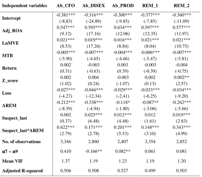
of the five measures for abnormal REM activities: the dependent variables Ab_CFO, Ab_PROD, Ab_DISEX and aggregate measures of real earnings management; REM_1 and REM_2. The coefficients on AREM capture the main effects of abnormal REM activities on future performance. “Suspect” is defined as an indicator variable for suspect firm-years just meeting earnings benchmarks (i.e., zero benchmarks and last year’s benchmarks). Suspect*AREM is an interaction term that captures the incremental effects of abnormal REM activities in the presence of meeting earnings benchmarks. Finally, to capture the total “value destroying” and “signalling” impacts of REM activities, we test the sum of the coefficient on AREM, (𝛂7) and the coefficient on the interaction terms of firms in the presence of just meeting earnings benchmarks Suspect*AREM, (𝛂9).
3.5. Measurements of control variables
To avoid the problem of correlated omitted variables, we base our main set of control variables on prior studies that suggest several factors that affect future operating performance (e.g., Gunny, 2010; Taylor and Xu, 2010; Zhao et al., 2012; Leggett et al., 2016). To be consistent with the dependent variable, all continuous independent variables are industry-adjusted.10 The potential influence of a size effect is controlled by adding firm size (LnMVE)
9 In sensitivity analyses, we also examine two- and three-year-ahead performance and check the results with an
alternative firm’s performance variable (industry-adjusted return on equity).
17
to the regression model, calculated as the natural logarithm of market capitalisation. Fama and French (1992) demonstrate that market capitalisation offers an important representation of the future expectations of the firm. To control for the life cycle of the firm, growth opportunities are included in the regression models as a control variable because Fama and French (1992) note that growth opportunities are a direct signal of the relative future prospects of firms and are calculated as the ratio of the market value of common equity divided by the book value of equity or market-to-book (MTB) ratio. Following Zang (2012), the current study uses the bankruptcy prediction model developed by Altman (1968, 2000), which is represented here by the Altman Z_score, to control for the financial health of the firm. A higher Z_score implies a firm’s healthier financial condition, and a lower Z_score implies poorer financial condition of firms.11
Loss is measured as the indicator variable equal to one when net income before extraordinary items is negative and zero otherwise and is included in the model because earnings are less persistent for firms with negative income.12 We also include the current-period
industry-adjusted financial profitability to control for the time-series properties (i.e., persistence) of performance. However, previous research demonstrates that there is a significantly positive association between one-year-ahead earnings and past-period earnings (Sloan, 1996; Dechow et al., 2003; Kraft et al., 2007, Gunny, 2010; Taylor and Xu, 2010). Following Kothari and Sloan (1992) and Gunny (2010), to control for the association between stock performance and future net income, market-adjusted abnormal returns is a proxy for the firm’s market performance. This is included in the regression models as a control variable,
11 The Altman Z_score model is Z_score = 0.3*(X1) + 1.0*(X2) + 1.4*(X3) + 1.2*(X4) + 0.6*(X5), where Z_score
represents the Altman (1968, 2000) distress score with which the relative financial condition of the firm can be explained based on magnitude and sign, measured at the beginning of year t. X1 represents the net income before extraordinary items are added to the total assets ratio. X2 represents the total sales to the total assets ratio. X3 represents the retained earnings to the total assets ratio. X4 represents the working capital to the total assets ratio. X5 represents the market value of equity to the total liabilities ratio.
12 Roychowdhury (2006) finds evidence that firms with higher net incomes are less likely to manage earnings and
18
calculated as the difference between monthly buy-and-hold raw returns and the monthly market buy-and-hold return, compounded over 12 months of the fiscal year t.13
4.
Empirical results
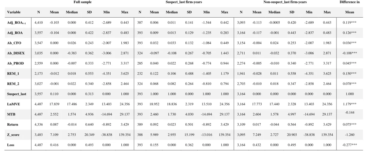
4.1. Descriptive statistics and correlations
Table 2 (Panel A and Panel B) presents the descriptive statistics for all variables in the empirical models comparing suspect firm-years just meeting zero earnings and last year’s earnings with the non-suspect firm-years. The mean industry-adjusted return on assets (ROA) are -10.3% and -10.4% for the subsequent dependent variable (Adj_ROAt+1) and current year
industry-adjusted return on assets (Adj_ROA), respectively. The medians for both are, on average, zero, which is estimated because the variables are calculated by deducting the industry-year median from the firms’ perceived return on assets.
The suspect firm-years in Panel A and Panel B have significantly lower values for Ab_DISEX than non-suspect firm-years, which suggests that suspect firm-years around zero earnings and last year’s earnings with low discretionary expenses engage more in real activity manipulation. In contrast, in Panel A, the mean REM_1 and REM_2 of suspect firm-years have significantly higher means than non-suspect firm-years, suggesting that the firm also engages in real activity manipulation. The mean Ab_CFO and Ab_PROD of suspect firm-years around zero earnings have a higher mean, although this is not significant compared to non-suspect firm-years. In addition, in Table 2 (Panel B), the mean of Ab_CFO, Ab_PROD, REM_1 and REM_2 of the suspect firm-years have a significantly higher mean than the means for the non-suspect firm-years. This suggests that non-suspect firm-years that just meet benchmarks around last year’s earnings engage in real activity manipulation.
13 Consistent with Bens et al. (2002), this examination uses the 12 months buy-and-hold stock return on the firm’s
ordinary shares. Gunny (2010, p. 877) computes size-adjusted abnormal returns as “the monthly buy and hold raw return minus the monthly buy and hold return on a size matched decile portfolio of firms compounded over 12 months of fiscal year t”.
19
The mean of Z_score is 7.109, with a median of 2.753, above the cut-off point (1.80: Altman, 1968, 2000) of being a healthy firm. These values are comparable to those in Zang (2012). The mean of Loss is 0.416 with a median of zero. Approximately 41.6% of the sample observations experienced losses, suggesting that firms might have the potential to engage in real manipulation. Finally, consistent with prior literature (e.g., Roychowdhury, 2006; Cohen et al., 2008; Gunny, 2010; Zhao et al., 2012; Leggett et al., 2016), suspect and non-suspect firm-years around zero earnings and last year’s earnings are different in numerous financial aspects.
Table 3 provides information about the Pearson and the Spearman correlation coefficients of all variables in the future operating performance regression. Adj_ROAt+1 is
significantly negatively related to three of the five REM measures except REM_1, Ab_DISEX, indicating that the main effects of abnormal REM activities on the firm in the absence of just meeting important earnings benchmarks is that they perform worse in the future or in signalling future performance. However, this reduces the firm’s value which will harm the firm’s future performance (value destroying), which is comparable to the findings of prior studies. Addressing the correlation coefficients above 0.60 specifically, the Adj_ROAt+1 is significantly
positive with a current year-adjustedreturn on assets (Pearson 66%, Spearman 70%), which is expected because of earnings persistence.
The current and one-year-ahead industry-adjusted return on assets are significantly positively correlated with firm size (Pearson 33%, 30%, respectively and Spearman 43%, 46%, respectively). This supports the assumption that firms have better current and future performance. The subsequent year’s industry-adjusted returns on assets have a strong negative correlation with the firms that experience negative net income (Loss), although this is significant (Pearson -38.5% and Spearman -50%).
20
The analysis of the correlation among the REM activity proxies reveals that the correlation between Ab_PROD and Ab_DISEX is significantly positive (Pearson 35.5% and Spearman 52%). This suggests that managers are using real activity manipulation, which leads to abnormally high production costs that occur simultaneously with reducing discretionary expenditures (Gunny, 2010; Zang, 2012). There is a significant negative relationship between Ab_DISEX and Ab_CFO (Pearson -43%, Spearman -17%); this shows that reduction of discretionary expenses frees up more cash flow for the firm. This result is consistent with prior research (e.g., Cohen et al., 2008; Cohen and Zarowin, 2010). In addition, the positive and significant correlation coefficient (34%, Pearson and 42%, Spearman) between Ab_CFO and Ab_PROD shows that (a) UK firms could engage in different REM methods at the same time to trigger higher reported earnings, and (b) it has a negative effect on cash flow from operations. Furthermore, the higher correlation coefficients of abnormal REM and the aggregate measures of REM (REM_1, REM_2) are expected because these aggregate measures of REM are the sum of two proxies, suggesting that firms engage in real activity manipulation, which is consistent with prior research (Zang, 2012). Finally, the mean variance inflation factors (VIF) for the independent variables used in the regression analysis of subsequent operating performance of firms just meeting zero earnings and last year’s earnings, for all five measures of REM, are all less than 1.50, suggesting that multicollinearity is not a concern in this study. 4.2. Main results
Table 4 reports the mean coefficient estimates from the Fama-MacBeth regressions. The t-statistics are calculated using standard errors corrected for autocorrelation using the Newey-West procedure. Table 4 (Panels A and B) reports a regression explaining the dependent variable (Adj_ROA t+1) over the subsequent one year using the proxies of the REM methods. The coefficients’ estimate for Adj_ROA is significantly different from zero and positive in each of the REM methods. This indicates that current-period industry-adjusted financial
21
profitability is positively associated with future industry-adjusted ROA (p-value < 0.01), which is consistent with the findings from prior empirical studies in the US (e.g., Gunny, 2010; Leggett et al., 2016).
The signs and significance of the control variables are consistent with the results from prior studies (e.g., Gunny, 2010; Taylor and Xu, 2010; Zhao et al., 2012 and Leggett et al., 2016) with only a few exceptions. The coefficients’ estimate on LnMVE is significantly different from zero and positive in each of the REM methods, indicating that suspect firm-years to meet zero earnings and last year’s earnings have better future performance, which is consistent with the findings of Gunny (2010) and Leggett et al. (2016). The coefficients’ estimate on MTB is statistically significant at the 0.01 level and is negative in each of the REM methods. This indicates that growth firms underperform in the future, which is consistent with the findings of Gunny (2010).
The coefficient estimates on Loss in each of the REM methods of the regression model are all significantly negatively associated with future performance (p-value < 0.01). This indicates that firms that engage in REM activities in the absence of meeting earnings benchmarks perform worse in the future or in signalling future performance compared to other firm-years. Zang (2012) points out that future profitability will be more negatively affected by REM activities when firms are in poor financial health, whereas coefficients on the Z_score are not significant in each of the REM methods, except for the coefficient on aggregate measures of real earnings management (REM_2), which is positive and statistically significant at 0.002 (t = 2.69) at the 1% level. This finding is in line with a prior empirical study by Gunny (2010). On the other hand, no coefficients on return significantly provide information about possible future performance.
Gunny (2010, p. 860) notes that “When examining the relation between future performance and RM, I assume RM is an exogenous variable. If RM is endogenously
22
determined such that there is a factor that affects RM and also affects firms’ future performance (e.g., RM firm-years being representative of poor performance), then this study suffers from a potential correlated omitted variable problem”. Therefore, we carefully control for the endogenous relationships between REM and firm future performance with a focus on REM; this focus is conditional upon an earnings management incentive, which is to guard against the effects of conflicting explanations and the possibility of the omission of correlated variables. However, Hypothesis 1 focuses on firms that manipulate their sales, discretionary expenses and production in the presence of meeting earnings benchmarks beyond the expanded focus on all firms that engage in REM. Hence, the coefficient of interest 𝛂9 represents the performance of Suspect firms that is augmented with REM measures compared to other firms.
The interaction term (Suspect*AREM) in the first three columns of Table 4 (Panels A and B), which captures the incremental effects of abnormal REM activities in the presence of meeting zero earnings and last year’s earnings, is significantly positively associated with future operating performance at the 0.01 significance level, which is consistent with Gunny’s (2010) and Zhao et al.’s (2012) findings; this suggests that managers who engage in REM to meet zero earnings and last year’s earnings through sales-based manipulation, discretionary expenses, and overproduction have better subsequent performance than other firm-years. They also convey a signal of superior future performance to the market. In the last two columns of Table 4, Panels A and B report the results from the regression model with aggregate REM measures. The average coefficients on the two aggregate REM measures, Suspect_zero*REM_1 and Suspect_zero*REM_2, are positive and statistically significant at 0.211 (t = 2.86) and 0.540 (t = 4.30), respectively. Additionally, the average coefficients on the two aggregate REM measures, Suspect_last*REM_1, Suspect_last*REM_2, are positive and statistically significant at 0.148 (t = 3.10) and 0.343 (t = 4.99), respectively. Hence, these results confirm that to meet zero earnings and last year’s earnings, managers of suspect firm-years who
23
simultaneously engage in discretionary expenses-based manipulation, production costs-based manipulation, sales-based manipulation and discretionary expenses-based manipulation have better subsequent operating performance.
Furthermore, the results of the AREM coefficients indicate that the main effects of abnormal REM activities are all negative and significant (p-value < 0.01). This is comparable to the findings of prior studies (Roychowdhury, 2006; Cohen and Zarowin, 2010) and suggests the general value destroying of the shareholders’ effect of abnormal REM activities in the absence of meeting earnings benchmarks. In other words, firms that do not meet zero earnings and firms that do not sustain recent performance but engage in REM activities perform worse in the future or in signalling future performance than other firm-years.
Regarding the joint signalling effect documented by Gunny in her 2010 study, she reports that firms that utilise REM to meet earnings benchmarks exhibit significantly better future performance than other REM firms that miss the targets, jointly signalling to the market that these firms perform better. As shown in Table 4 (Panel A), however, the results of the sum of
𝛂7 and 𝛂9, which captures the combined “value-destroying” and “signalling” impacts of REM activities, show that the term (𝛂7 + 𝛂9) is significantly positive for three of five measures of REM — Ab_DISEX, Ab_PROD, and REM_2 (p-value < 0.1 or p-value < 0.01). This indicates that just to meet zero earnings, firm-years with engagement in REM activities have better subsequent operating performance (have significantly higher industry-adjusted ROA) than other firm-years with abnormal REM activities. This result is consistent with joint signalling; that is, engaging in REM activities in the presence of meeting the important earnings benchmarks to signal superior future performance (e.g., Gunny, 2010; Zhao et al., 2012).
In Panel B of Table 4, the results of the sum of the coefficients Suspect_last*AREM, 𝛂9 and AREM show that 𝛂7 is significantly positive for one of five measures of REM (Ab_PROD) analyses at the 0.05 significance level. This indicates that firm-years to just meet last year’s
24
earnings that engage in REM activities have better subsequent operating performance than other firm-years with abnormal REM activities. In addition, in the case of Ab_DISEX, the sum of coefficients 𝛂7 (-0.338) and 𝛂9 (0.171) is -0.166. The Wald test t-values of 𝛂7 and 𝛂9 are significantly negative at the 0.05 significance level (t = -2.18), indicating that firm-years that engage in REM to meet last year’s earnings perform worse in the future or in signalling future performance than other firm-years with abnormal REM activities.
4.3. Robustness checks
4.3.1. The sensitivity of the results to the period of two-year and three year-ahead industry-adjusted return on assets
The results in Table 5 (Panel A and B) reveal that, in general, are robust when using Adj_ROAt+2 as the future performance measure and are consistent with the results from
Adj_ROAt+1 in Table 4 (Panel A and Panel B). For example, four of the five interaction terms
of the suspect firm-years of all measures of REM remain the same, and all are significantly positively associated with future operating performance in year two at the 0.01 significance level. The Ab_CFO that interacted with suspect firm-years (Suspect_zero, Suspect_last) are still significantly positive, where the significance levels drop from 1% to 5% and 10%, respectively. The significance levels also drop from 1% to 5% on the coefficient of Ab_DISEX*Suspect_last; however, it shows no significant differences.
The main effects of all abnormal REM activities remain the same, and all are negative and significant with future operating performance in year two at the 0.01 significance level. In addition, the combined coefficients on the interaction terms of abnormal REM (𝛂7, 𝛂9), which represents the full impact of REM on a firm’s subsequent two-year operating performance, are also positive and significant at the 0.01 significance level in the abnormal production cost analysis. However, the combined coefficients are negative and statistically significant at the 0.05 significance level in the abnormal discretionary expenses analysis. Furthermore, the other
25
combined coefficients of 𝛂7 and 𝛂9 maintain the same sign but are no longer statistically significant. Overall, the results generally remain unchanged, suggesting that our findings are robust to the subsequent operating performance in year two as well as in their performance in year one.14
5.
Conclusions
In this study, we focus on a sample of firms listed on the LSE to examine whether there is an association between UK firms that manipulate their sales, discretionary expenses and production to just meet certain earnings benchmarks and future operating performance. Our regression results show that UK firms that manipulate their earnings to meet zero earnings and last year’s earnings are all significantly positively associated with future operating performance, which is consistent with Gunny’s (2010) and Zhao et al.’s (2012) findings and suggests that abnormal REM is intended to meet zero earnings and last year’s earnings and transmit a signal of superior future performance to the market. Furthermore, the results also show that UK firms that manipulate their earnings are all negatively associated with future operating performance, which is comparable to the findings of prior studies (Gunny, 2010; Zhao et al., 2012). These results suggest a general value destroying outcome of shareholders’ effect of abnormal REM activities in the absence of just meeting important benchmarks.
When drawing evidence-based conclusions, consideration should be paid to some limitations identified in this study. One limitation of this study is that we only investigated motivation for REM, which is to meet important earnings benchmarks, such as avoiding report losses and sustaining recent profit performance. In reality, many other factors could drive earnings management such as compensation contracts, avoiding violations of debt covenants,
14 The untabulated results reveal that, in general, are robust when using Adj_ROA t+3 as the future performance
measure, consistent with the results from Adj_ROAt+1 Adj_ROAt+2. However, the results remain unchanged for
three-year-ahead, suggesting that our findings are also robust to the subsequent operating performance in year three as well as in their performance in years one and two.
26
and investors when managers are generating their financial reports. The second limitation is that there is a variety of factors not investigated in this research that can influence REM in a number of ways: for example, audit quality, corporate governance or disclosure policies are less likely to engage in earnings management. Another limitation with the present study is that it examines the manipulation of common business activities, such as sales, discretionary expenditures and production, but does not investigate other measures of earnings management, such as underinvestment in long-term projects, discretionary investment in R&D, abnormal gains on sales of fixed assets and accrual earnings management. Finally, because this study focuses on UK data, due to data access limitations, we do not explore the factors mentioned above, which are considered important areas in the earnings management literature.
Appendices
Appendix A Proxies for abnormal real earnings management activities.
The first measure for REM activities is the abnormal cash flows from operations (Ab_CFO). Following previous studies (e.g., Roychowdhury, 2006; Cohen et al., 2008; Cohen and Zarowin, 2010; Badertscher, 2011), sales-based manipulations are expected to lead to decreased current-period operating cash flows. We express the normal cash flows from operations as a linear function of sales revenue and change in sales revenue in the current period using the model developed by Dechow et al. (1998) as implemented in Roychowdhury (2006).
27
To estimate this model, we run the following cross-sectional regression for each industry and year for all firms listed on the London Stock Exchange (LSE):
𝐶𝐹𝑂𝑖,𝑡 𝑇𝐴𝑖,𝑡−1 = 𝛼0+ 𝛽1∗ ( 1 𝑇𝐴𝑖,𝑡−1) + 𝛽2∗ ( 𝑆𝐴𝐿𝐸𝑆𝑖,𝑡 𝑇𝐴𝑖,𝑡−1) + 𝛽3∗ ( ∆𝑆𝐴𝐿𝐸𝑆𝑖,𝑡 𝑇𝐴𝑖,𝑡−1 ) + 𝜀𝑖,𝑡, (A-1)
where 𝐶𝐹𝑂𝑖,𝑡is cash flows from operations for firm 𝑖 in the year 𝑡, defined as cash flows from
operations divided by lagged total assets; TAi,t-1 is the total assets at the beginning of period 𝑡
for firm 𝑖; 𝑆𝐴𝐿𝐸𝑆𝑖,𝑡 is the sales revenue during period 𝑡 for firm 𝑖; ∆𝑆𝐴𝐿𝐸𝑆𝑖,𝑡 is the change in
sales revenue from year 𝑡 − 1 to 𝑡; 𝑖 is the firm; and 𝜀𝑖,𝑡 is the error term. For every firm on the
LSE, Ab_CFO is computed as actual cash flows from operations minus the normal level of cash flows from operations predicted from equation (A-1).
Another measure for REM activities is abnormal discretionary expenses (Ab_DISEX). Following previous studies (e.g., Roychowdhury, 2006; Cohen et al., 2008; Cohen and Zarowin, 2010; Badertscher, 2011; Zang, 2012), we model discretionary expenses as a linear function of lagged sales and then estimate the following model to derive the normal levels of discretionary expenses for all firms listed on the LSE cross-sectionally for each industry and year, 𝐷𝐼𝑆𝐸𝑋𝑖,𝑡 𝑇𝐴𝑖,𝑡−1 = 𝛼0 + 𝛽1∗ ( 1 𝑇𝐴𝑖,𝑡−1) + 𝛽2∗ ( 𝑆𝐴𝐿𝐸𝑆𝑖,𝑡−1 𝑇𝐴𝑖,𝑡−1 ) + 𝜀𝑖,𝑡, (A-2)
where 𝐷𝐼𝑆𝐸𝑋𝑖,𝑡 is the discretionary expenses that are defined as the sum of R&D, advertising, and selling, general and administrative expenses in year 𝑡 for firm 𝑖; and 𝑆𝐴𝐿𝐸𝑆𝑖,𝑡−1 is the sales
revenue at the beginning of year 𝑡 for firm 𝑖. For every firm on the LSE, the Ab_DISEX is computed as the difference between the actual discretionary expenses and the normal level of discretionary expenses.
The third measure of REM activities is abnormal production costs (Ab_PROD). Studies such as Roychowdhury (2006), Cohen et al. (2008), Gunny (2010), Cohen and Zarowin (2010),
28
Badertscher (2011), and Zang (2012) define production costs as the sum of the cost of goods sold and change in inventory during the year, and they express the normal level of production costs as a linear function of contemporaneous sales. Following these studies, we estimate the following model for normal production costs,
𝑃𝑅𝑂𝐷𝑖,𝑡 𝑇𝐴𝑖,𝑡−1 = 𝛼0+ 𝛽1∗ ( 1 𝑇𝐴𝑖,𝑡−1 ) + 𝛽2∗ ( 𝑆𝐴𝐿𝐸𝑆𝑖,𝑡 𝑇𝐴𝑖,𝑡−1 ) + 𝛽3∗ ( ∆𝑆𝐴𝐿𝐸𝑆𝑖,𝑡 𝑇𝐴𝑖,𝑡−1 ) + 𝛽4∗ ( ∆𝑆𝐴𝐿𝐸𝑆𝑖,𝑡−1 𝑇𝐴𝑖,𝑡−1 ) + 𝜀𝑖,𝑡, (A-3)
where 𝑃𝑅𝑂𝐷𝑖,𝑡 is the sum of the cost of goods sold in year 𝑡 for firm 𝑖 and the change in inventory from 𝑡 − 1 to 𝑡; and ∆𝑆𝐴𝐿𝐸𝑆𝑖,𝑡−1 is the change in sales revenue at the beginning of
year 𝑡 for firm 𝑖. The Ab_PROD is computed as the difference between the actual values of production costs and the normal levels predicted from equation (A-3). Equation (A-3) is estimated as cross-sectional for each industry and year.
29
Variable Definition/Measurement Data sources
TA = Total assets (WC02999). Worldscope
SALES = Sales revenue (WC01001). Worldscope
IBEI = Income before extraordinary items (WC01551). Worldscope
CFO = Cash flows from operations (WC04860). Worldscope
COGS = Cost of goods sold (WC01051). Worldscope
INV = Inventories (WC02101). Worldscope
PROD = Production costs; the sum of cost of goods sold and change in inventory.
R&D = Research and development expenses (WC01201). Worldscope
ADV and SG&A = Advertising and selling, general and administrative expenses (WC01101). Worldscope DISEX = Discretionary expenses; the sum of R&D, ADV and SG&A.
Ab_CFO = Abnormal cash flows from operations, where Ab_CFO is measured by the estimated residual from the regression equation (A-1). Ab_DISEX = Abnormal discretionary expenses, where Ab_DISEX is measured by the estimated residual from the regression equation (A-2). Ab_PROD = Abnormal production costs, where Ab_PROD is measured by the estimated residual from the regression equation (A-3).
REM_1 = The sum of Ab_DISEX*(-1) and Ab_PROD; the higher the values of this aggregate measure are, the more likely it is that the firm is engaging in real activity manipulation.
REM_2 = The sum of Ab_CFO*(-1) and Ab_DISEX*(-1); the higher the values of this aggregate measure are, the more likely it is that the firm is engaging in real activity manipulation.
ROA = Return on assets; income before extraordinary items scaled by lagged total assets.
MTB = Market-to-book; the ratio of market value of equity (WC08001) to book value of equity (WC03501), measured at the beginning of year t.
Worldscope
LnMVE = Logarithm of the market value of equity, measured at the beginning of year t.
Suspect = An indicator variable for suspect firm-years just meeting/beating important earnings benchmarks.
Suspect_zero = An indicator variable that is set equal to one if net income before extraordinary items scaled by lagged total assets is between 0 and 0.005 and is set equal to zero otherwise, based on Roychowdhury’s (2006) criteria to identify suspect firm-years.
Worldscope
Suspect_last = An indicator variable that is set equal to one if the change in net income before extraordinary items from the last year is between 0 and 0.01 and is set equal to zero otherwise, based on Gunny’s (2010) criteria to identify suspect firm-years.
Loss = An indicator variable equal to one when the net income before extraordinary items is negative and zero otherwise.
Return = Market-adjusted abnormal returns are a proxy for the firm’s market performance, calculated as the difference between monthly buy-and-hold raw returns and the monthly market buy-buy-and-hold returns, compounded over 12 months of the fiscal year t.
Datastream
Z_score = Measures the financial strength at the beginning of year t, computed as 0.3*(IBEI/TA) + 1.0*(SALES/TA) + 1.4*(Retained earnings (WC03495)/TA) + 1.2*(Working capital (WC03151)/TA) + 0.6*(Market value of equity/Total liabilities (WC03351)).
Worldscope
Adj_ROAt+1 = One-year-ahead industry-adjusted financial performance return on assets, calculated as the differences between firm-specific ROA
and median ROA for the same year and industry (2-digit SIC code) as a direct measure of the firm’s longer-term cash flow.
ROE = Return on equity is the ratio of net income before extraordinary items divided by common equity. (WC08301). Worldscope Adj_ROEt+1 = One-year-ahead industry-adjusted financial performance return on equity, calculated as the differences between firm-specific ROE
30
References
Alhadab, M., Clacher, I., & Keasey, K. (2015). Real and accrual earnings management and IPO failure risk. Accounting and Business Research, 45(1), 55-92.
Altman, E. (1968). Financial ratios, discriminate analysis and the prediction of corporate bankruptcy. Journal of Finance, 23(4), 589-609.
Altman, E. (2000). Predicting financial distress of companies: Revisiting the Z-score and ZETA models. Working paper, New York University.
Baber, W., Fairfield, P., & Haggard, J. (1991). The effect of concern about reported income on discretionary spending decisions: The case of research and development. The Accounting Review, 66(4), 818-829.
Badertscher, B. (2011). Overvaluation and the choice of alternative earnings management mechanisms. The Accounting Review, 86(5), 1491-1518.
Ball, R., Kothari, P., & Ashok, R. (2000). The effect of international institutional factors on properties of accounting earnings. Journal of Accounting and Economics, 29(1), 1-51. Barton, J., & Simko, P. (2002). The balance sheet as an earnings management constraint. The
Accounting Review, 77, 1-27.
Bartov, E., Givoly, D., & Hayn, C. (2002). The rewards to meeting or beating earnings expectations. Journal of Accounting and Economics, 33(2), 173-204.
Bens, D., Nagar, V., & Wong, M. (2002). Real investment implications of employee stock option exercises. Journal of Accounting Research, 40(2), 359-393.
Bhojraj, S., & Libby, R. (2005). Capital market pressure, disclosure frequency-induced earnings/cash flow conflicts, and managerial myopia. The Accounting Review, 8(1), 1-20. Bhojraj, S., Hribar, P., Picconi, M., & McInnis, J. (2009). Making sense of cents: An examination of firms that marginally miss or beat analyst forecasts. The Journal of Finance, 64(5), 2359-2386.
Brown, L., & Higgins, H. (2001). Managing earnings surprises in the US Versus 12 other countries. Journal of Accounting and Public Policy, 20(4/5), 373-398.
Brown, L., & Higgins, H. (2005). Managers’ forecast guidance of analysts: International evidence. Journal of Accounting and Public Policy, 24(4), 280-299.
Burgstahler, D., & Dichev, I. (1997). Earnings management to avoid earnings decreases and losses. Journal of Accounting and Economics, 24(1), 99-126.
Cohen, D., Dey, A., & Lys, T. (2008). Real and accrual-based earnings management in the pre- and post-sarbanes-oxley periods. The Accounting Review, 83(3), 757-787.
Cohen, D., & Zarowin, P. (2010). Accrual-based and real earnings management activities around seasoned equity offerings. Journal of Accounting and Economics, 50, 2-19.
De Jong, A., Merten, G., van der Poel, M., & van Dijk, R. (2014). How does earnings management influence investor’s perceptions of firm value? Survey evidence from financial analysts. Review of Accounting Studies, 19(2), 606-627.
Dechow, P., & Dichev, I. (2002). The quality of accruals and earnings: The role of accrual estimation errors. The Accounting Review, 77(1), 35-59.
Dechow, P., Ge, W., & Schrand, C. (2010). Understanding earnings quality: A review of the proxies, their determinants and their consequences. Journal of Accounting and Economics, 50(2/3), 344-401.
Dechow, P., Kothari, S., & Watts, R. (1998). The relation between earnings and cash flows. Journal of Accounting and Economics, 25, 133-168.
Dechow, P., Richardson, S., & Tuna, I. (2003). Why are earnings kinky? An examination of the earnings management explanation. Review of Accounting Studies, 8(2), 355-384.
31
DeFond, M., & Park, C. (1997). Smoothing income in anticipation of future earnings. Journal of Accounting and Economics, 23(2), 115-139.
Degeorge, F., Patel, J., & Zeckhauser, R. (1999). Earnings management to exceed thresholds. The Journal of Business, 72(1), 1-33.
Demski, J. (1998). Performance measure manipulation. Contemporary Accounting Research, 15(3), 261-285.
Eldenburg, L., Gunny, K., & Soderstrom, N. (2011). Earnings management using real activities: Evidence from nonprofit hospitals. The Accounting Review, 86(5), 1605-1630.
Ewert, R., & Wagenhofer, A. (2005). Economic effects of tightening accounting standards to restrict earnings management. The Accounting Review, 80(4), 1101-1124.
Fama, E., & French, K. (1992). The cross-section of expected stock returns. The Journal of Finance, 47(2), 427-465.
Fama, E., & MacBeth, J. (1973). Risk, return, and equilibrium: Empirical tests. Journal of Political Economy, 81(3), 607-636.
Francis, B., Hasan, I., & Li, L. (2016a). Abnormal real operations, real earnings management, and subsequent crashes in stock prices. Review of Quantitative Finance and Accounting, 46(2), 217-260.
Francis, B., Hasan, I., & Li, L. (2016b). A cross-country study of legal-system strength and real earnings management. Journal of Accounting and Public Policy, 35(5), 477-512.
Ge, W., & Kim, J-B. (2014). Real earnings management and the cost of new corporate bonds. Journal of Business Research, 67(4), 641-647.
Graham, J., Harvey, C., & Rajgopal, S. (2005). The economic implications of corporate financial reporting. Journal of Accounting and Economics, 40, 3-73.
Gunny, K. (2010). The relation between earnings management using real activities manipulation and future performance: Evidence from meeting earnings benchmarks. Contemporary Accounting Research, 27(3), 855-888.
Han, S., Kang, T., Salter, S., & Yoo, Y. (2010). A cross-country study on the effects of national culture on earnings management. Journal of International Business Studies, 41(1), 123-141.
Harrell, F. (2015). Regression modeling strategies with applications to linear models, logistic and ordinal regression, and survival analysis, (2nd ed.). New York.
Healy, P., & Palepu, K. (1993). The effect of firms’ financial disclosure strategies on stock prices. Accounting Horizons, 7(1), 1-11.
Healy, P., & Wahlen, J. (1999). A review of the earnings management literature and it’s implications for standard setting. Accounting Horizons, 13(4), 365-383.
Hirshleifer, D., Kewei, H., Teoh, S., & Zhang, Y. (2004). Do investors overvalue firms with bloated balance sheets? Journal of Accounting and Economics, 38, 297-331.
Kim, J-B., & Sohn, B. (2013). Real earnings management and cost of capital. Journal of Accounting and Public Policy, 32(6), 518-543.
Koh, K., Matsumoto, D., & Rajgopal, S. (2008). Meeting or beating expectations in the post-scandals world: Changes in stock market rewards and managerial actions. Contemporary Accounting Research, 25(4), 1067-1098.
Kothari, S., Mizik, N., & Roychowdhury, S. (2016). Managing for the moment: The role of real activity versus accruals earnings management in SEO valuation. The Accounting Review, 91(2), 559-586.
Kothari, S. (2001). Capital markets research in accounting. Journal of Accounting and Economics, 31(1/3), 105-231.
Kothari, S., & Sloan, R. (1992). Information in prices about future earnings: Implications for earnings response coefficients. Journal of Accounting and Economics, 15(2/3), 143-171.